Israel Gelfand, who made profound and prolific contributions to many areas of mathematics, including functional analysis, representation theory, operator algebras, and partial differential equations, died on Monday, age 96.
Gelfand’s beautiful theory of  -algebras and related spaces made quite an impact on me as a graduate student in Princeton, to the point where I was seriously considering working in this area; but there was not much activity in operator algebras at the time there, and I ended up working in harmonic analysis under Eli Stein instead. (Though I am currently involved in another operator algebras project, of which I hope to be able to discuss in the near future. The commutative version of Gelfand’s theory is discussed in these lecture notes of mine.)
I met Gelfand only once, in one of the famous “Gelfand seminars” at the IHES in 2000. The speaker was Tim Gowers, on his new proof of Szemerédi’s theorem. (Endre Szemerédi, incidentally, was Gelfand’s student.) Gelfand’s introduction to the seminar, on the subject of Banach spaces which both mathematicians contributed so greatly to, was approximately as long as Gowers’ talk itself!
There are far too many contributions to mathematics by Gelfand to name here, so I will only mention two. The first are the Gelfand-Tsetlin patterns, induced by an  Hermitian matrix
  . Such matrices have
  real eigenvalues
 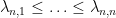 . If one takes the top
  minor, this is another Hermitian matrix, whose
  eigenvalues
  intersperse the eigenvalues of the original matrix:
 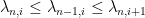 for every
  . This interspersing can be easily seen from the minimax characterisation
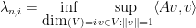
of the eigenvalues of , with the eigenvalues of the minor being similar but with  now restricted to a subspace of
  rather than
  .
.
Similarly, the eigenvalues  of the top
  minor of intersperse those of the previous minor. Repeating this procedure one eventually gets a pyramid of real numbers of height and width , with the numbers in each row interspersing the ones in the row below. Such a pattern is known as a Gelfand-Tsetlin pattern. The space of such patterns forms a convex cone, and (if one fixes the initial eigenvalues
  ) becomes a compact convex polytope. If one fixes the initial eigenvalues of but chooses the eigenvectors randomly (using the Haar measure of the unitary group), then the resulting Gelfand-Tsetlin pattern is uniformly distributed across this polytope; the
  case of this observation is essentially the classic observation of Archimedes that the cross-sectional areas of a sphere and a circumscribing cylinder are the same. (Ultimately, the reason for this is that the Gelfand-Tsetlin pattern almost turns the space of all with a fixed spectrum (i.e. the co-adjoint orbit associated to that spectrum) into a toric variety. More precisely, there exists a mostly diffeomorphic map from the co-adjoint orbit to a (singular) toric variety, and the Gelfand-Tsetlin pattern induces a complete set of action variables on that variety.) There is also a “quantum” (or more precisely, representation-theoretic) version of this observation, in which one can decompose any irreducible representation of the unitary group
  into a canonical basis (the Gelfand-Tsetlin basis), indexed by integer-valued Gelfand-Tsetlin patterns, by first decomposing this representation into irreducible representations of
  , then
  , and so forth.
The structure, symplectic geometry, and representation theory of Gelfand-Tsetlin patterns was enormously influential in my own work with Allen Knutson on honeycomb patterns, which control the sums of Hermitian matrices and also the structure constants of the tensor product operation for representations of ; indeed, Gelfand-Tsetlin patterns arise as the degenerate limit of honeycombs in three different ways, and we in fact discovered honeycombs by trying to glue three Gelfand-Tsetlin patterns together. (See for instance our Notices article for more discussion. The honeycomb analogue of the representation-theoretic properties of these patterns was eventually established by Henriques and Kamnitzer, using  crystals and their Kashiwara bases.)
The second contribution of Gelfand I want to discuss is the Gelfand-Levitan-Marchenko equation for solving the one-dimensional inverse scattering problem: given the scattering data of an unknown potential function  , recover . This is already interesting in and of itself, but is also instrumental in solving integrable systems such as the Korteweg-de Vries equation, because the Lax pair formulation of such equations implies that they can be linearised (and solved explicitly) by applying the scattering and inverse scattering transforms associated with the Lax operator. I discuss the derivation of this equation below the fold.
— 1. Inverse scattering —
Let  be a smooth real potential function supported on a compact interval
 ![{[-R,R]}](https://s0.wp.com/latex.php?latex=%7B%5B-R%2CR%5D%7D&bg=ffffff&fg=000000&s=0&c=20201002) (for simplicity), and consider the potential wave equation in one spatial dimension
(for simplicity), and consider the potential wave equation in one spatial dimension

for the scalar field  . If the potential was zero, then (1) becomes the free wave equation, the general solution
  of (1) would be the superposition of a rightward moving wave
  and a leftward moving wave
  :
:

Now suppose is non-zero. Then in the left region  ,
,  solves the free wave equation and thus takes the form

for some  , while in the right region
  , solves the free wave equation and takes the form

for some  . As for the central region
  , we will make the simplifying assumption that the equation (1) has no bound states, which implies in particular that
  as
as  for any fixed
  and any reasonable (e.g. finite energy will do). From spectral theory, this assumption is equivalent to the assertion that the Hill operator (or Schrödinger operator)
  has no eigenfunctions in
  .) Thus the wave is asymptotically equal to
  for large negative times, then evolves to interact with the potential, then eventually is asymptotic to
  for large positive
  .
.
When is zero, we have  and
and  . For non-zero , the relationship between
  , and involves something called the reflection coefficients and transmission coefficients of . We will not define these just yet, but instead focus on two special cases. Firstly, consider the case when
  is the Dirac delta function and
  ; thus for large negative times, the wave consists just of a Dirac mass (or “photon”, if you will) arriving from the left, and this generates some special solution
  to (1) (a bit like the fundamental solution). (We will ignore the (mild) technical issues involved in solving PDE with data as rough as the Dirac distribution.) Evolving the wave equation (1), the solution
  eventually resolves to some transmitted wave
  (which should be some perturbation of the Dirac delta function) plus a reflected wave
  , which we will call
  . This function can be thought of as “scattering data” for the potential .
Next, we will consider the solution  to (1) for which and
  ; one can view this solution as obtained by reversing the roles of space and time, and evolving (1) from
  to
to  (with the potential now being a constant-in-space, variable-in-time potential rather than the other way around). One can construct this solution by the Picard iteration method, and using finite speed of propagation, one can show that
  is supported on the lower diagonal region
  , and is smooth except at the diagonal
  , where it can have a jump discontinuity. One can think of
  as a dual fundamental solution for the equation (1); it is also the Fourier transform of the Jost solutions to the eigenfunction equation (5).
We claim that the scattering data can be used to reconstruct the potential . This claim is obtained from two sub-claims:
- Given the scattering data , one can recover .
- Given , one can recover .
The second claim is easy: one simply substitutes  into (1). Indeed, if one compares the
  components of both sides, one sees that
To verify the first claim, we exploit the time translation and time reversal symmetries of (1). Since  is a solution to (1), the time-reversal
  is also a solution. More generally, the time translation
  is also a solution to (1) for any real number
  . Multiplying this by
  and integrating in , we see that the function

is also a solution to (1). Superimposing this with the solution , we see that

is also a solution to (1).
Now when  , vanishes; and so this solution (2) is equal to
  for . Thus, by uniqueness of the evolution of (1) (in the direction), (2) must match the fundamental solution . On the other hand, by finite speed of propagation, this solution vanishes when
  . We thus obtain the Gelfand-Levitan-Marchenko equation

For any fixed , this is a linear integral equation for , and one can use it to solve from given by inverting the integral operator  . (This inversion can be performed by Neumann series if is small enough, which is for instance the case when the potential is small; in fact, one can use scattering theory to show that this operator is in fact invertible for all without bound states, but we will not do so here.)
Now I’ll discuss briefly the relationship between the data and more traditional types of scattering data. We already have the fundamental solution , which equals  for and for which
  . By time translation, we have a solution
  for any
  , which equals
  for and for which . Multiplying this solution by
  for some frequency
  and then integrating in , we obtain the (complex) solution
to (1), which equals

for , and equals some function  for , where

On the other hand, we can write the solution (4) as  , where
  . This implies that must be a multiple of the plane wave
  , thus
  for some complex number
  . Substituting into (1), we see that
  is a generalised eigenfunction of the Schrödinger operator:
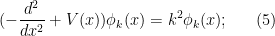
from the asymptotics of (4), we also see that 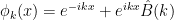 for and
 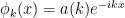 for
for  . Thus we see that
  has an interpretation as a reflection coefficient for the eigenfunction equation (5).


31 comments
Comments feed for this article
8 October, 2009 at 12:03 am
Jonas
Any recommendations for further reading on the general theory of Gelfand-Tsetlin patterns?
8 October, 2009 at 1:55 am
bruno
Thank you for this post (and the whole blog!). It seems that there is a typo when you introduce the solution $\delta(t-x)+K(t,x)$, hypothesis $g_+=0$ should perhaps be $g_-=0$ (consistent with considering $x$ as time). Am I wrong ?
[Oops, you’re right – corrected, thanks. -T.]
8 October, 2009 at 3:26 am
Stones Cry Out - If they keep silent… » Things Heard: e88v4
[…] A passing noted … and here’s a vivid demonstration of how memory is kept. […]
8 October, 2009 at 6:06 am
Allen Knutson
the Gelfand-Tsetlin pattern almost turns the space of all {A} with a fixed spectrum (i.e. the co-adjoint orbit associated to that spectrum) into a toric variety, though one first has to blow up a few singularities first to make this precise.
1) The action isn’t algebraic, so this isn’t a blowup in the usual complex algebraic sense.
2) It’s more of a blowdown, really. There’s a map from the coadjoint orbit onto the toric variety, whose fibers are isotropic. In the 3×3 case this map is a diffeomorphism away from the singular point on the toric variety, over which the fiber is a real-3-dimensional Lagrangian sphere.
8 October, 2009 at 7:23 am
Terence Tao
Ah, right, I had it backwards. (The coadjoint orbit is, of course, smooth for generic choices of the spectrum; it was the toric variety that had the singularity.) I’ve fixed the wording accordingly.
As an analyst, I guess I tend to think of blowups in the smooth category rather than the algebraic one, though it seems this meaning of the term is only used by a minority of mathematicians.
8 October, 2009 at 7:18 am
ramanujantao
Dear Terry,
Do you type your blog articles in say TeXnicCenter first? And then transfer them to your blog via Texter or some Perl script? Because when I first loaded the page I saw the following:
\documentclass[12pt]{article}
\usepackage[pdftex,pagebackref,letterpaper=true,colorlinks=true,pdfpagemode=none,urlcolor=blue,linkcolor=blue,citecolor=blue,pdfstartview=FitH]{hyperref}
\usepackage{amsmath,amsfonts}
\usepackage{graphicx}
\usepackage{color}
\setlength{\oddsidemargin}{0pt}
\setlength{\evensidemargin}{0pt}
\setlength{\textwidth}{6.0in}
\setlength{\topmargin}{0in}
\setlength{\textheight}{8.5in}
\setlength{\parindent}{0in}
\setlength{\parskip}{5px}
\input{macrosblog}
\begin{document}
8 October, 2009 at 7:24 am
Terence Tao
I use Luca Trevisan’s LaTeX to WP converter (a python script). I accidentally copied the source LaTeX here instead of the WP HTML by mistake for a few minutes.
8 October, 2009 at 7:28 am
ramanujantao
Dear Terry,
Here is a site which allows you to write LaTeX flies and convert them to pdf without installing MiKTeX or any editor: http://dev.baywifi.com/latex/
8 October, 2009 at 7:46 am
A semana nos arXivs… « Ars Physica
[…] Israel Gelfand […]
8 October, 2009 at 8:54 am
Kareem Carr
There is an article on Dr. Gelfand in the NYT:
“Israel Gelfand, Math Giant, Dies at 96”
8 October, 2009 at 9:23 am
Bill Watson
One should also mention Prof. Gelfand’s important contributions to the math education of gifted students in his program at Rutgers (no longer operational).
http://gcpm.rutgers.edu/former_description.html
8 October, 2009 at 1:19 pm
Israel Gelfand (1913-2009). R.I.P. « Successful Researcher
[…] learn more about him, see e.g. the excellent post by Terence […]
8 October, 2009 at 1:47 pm
Random bits « Equilibrium Networks
[…] Terry Tao reports that Israel Gelfand died recently. He was one of the greats, his name familiar to every student of functional analysis from the GNS […]
8 October, 2009 at 5:28 pm
Jake
Typo alert: Just after (1) you have “leftward moving moving wave” [Corrected, thanks – T.]
8 October, 2009 at 7:50 pm
Israel M. Gelfand (1913 – 2009) « Series Divergentes
[…] Israel Gelfand (What’s new, por Terry Tao) […]
9 October, 2009 at 1:53 am
mfrasca
Hi Terry,
I think there is a repetition here:
There are far too many contributions to mathematics by Gelfand to name here, so I will only mention only two.
Marco
[Corrected, thanks – T.]
9 October, 2009 at 12:42 pm
Short News Items « Not Even Wrong
[…] I. M. Gelfand died on Monday at the age of 96. For more about him, see here, here and here. […]
9 October, 2009 at 4:23 pm
Top Posts « WordPress.com
[…] Israel Gelfand Israel Gelfand, who made profound and prolific contributions to many areas of mathematics, including functional analysis […] […]
10 October, 2009 at 2:36 am
Israel M. Gelfand, uno de los matemáticos más importantes del s. XX, descanse en paz « Francis (th)E mule Science's News
[…] los matemáticos y físicos, recomiendo la entrada del genial Terence Tao, “Israel Gelfand,” What’s New, 7 October, 2009. Se centra en la ecuación de […]
12 January, 2010 at 9:03 pm
254A, Notes 3a: Eigenvalues and sums of Hermitian matrices « What’s new
[…] for all . (Hint: use the Courant-Fischer min-max theorem, Theorem 2.) Show furthermore that the space of for which equality holds in one of the inequalities in (24) has codimension (for Hermitian matrices) or (for real symmetric matrices. Remark 5 If one takes successive minors of an Hermitian matrix , and computes their spectra, then (24) shows that this triangular array of numbers forms a pattern known as a Gelfand-Tsetlin pattern. These patterns are discussed a little more in this blog post. […]
3 June, 2010 at 10:24 am
Vladimir Arnold (1937-2010). R.I.P. « Successful Researcher
[…] Vladimir Arnold (1937-2010). R.I.P. One of the world’s greatest and most influential mathematicians, Vladimir Arnold, passed away today in Paris, France. He made major contributions, inter alia, to the fields of dynamical systems (the famous KAM (Kolmogorov-Arnold-Moser) theory) and topology (he is one of the founding fathers of symplectic topology). I hope that the prominent mathematicians like Terence Tao or Timothy Gowers will say more on their blogs about Arnold’s scientific legacy as they did for Israel Gelfand. […]
1 September, 2013 at 11:49 pm
Centenario de Israel Gelfand | :: ZTFNews.org
[…] Israel Gelfand en la página de Terence Tao […]
1 September, 2016 at 11:48 pm
Israel Gelfand (1913-2009) |
[…] Israel Gelfand en la página de Terence Tao […]
28 May, 2018 at 1:42 pm
timo
I don’t understand how you get to the equation of V(x) in terms of K (by comparing the delta components of both sides), its probably a silly misunderstanding but I would be very grateful if you could lay it out for me. Thank you very much
29 May, 2018 at 9:58 am
Terence Tao
As discussed previously, the discontinuous function can be written as
 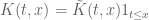 , where
  extends smoothly across the diagonal. Applying the differential operator
  to this distribution then gives (after using the Leibniz rule)
  plus some smooth terms; as
  solves the wave equation, the left-hand side of (1) also has this form. Meanwhile, the right-hand side of (1) is equal to
  plus smoother terms, giving the claim.
2 June, 2018 at 6:55 pm
YahyaAA1
Thanks for this post, Terry! Particularly for your insights into the motivations of these areas of Gelfand’s work. Timo’s question brought this blog post to my notice for the first time, as I only subscribed a few months ago.
Also, as ever, you generously answer difficulties such as Timo’s. :-)
Explanations in maths seem to fall into two styles, which I think of as “the ideas” and “the rigour”. The ideas explain why, and the rigour explains how. It’s great to start with the why! Some writers only operate at the level of technical, rigorous detail, which can leave us floundering seeking the why – shedding more darkness than light. That’s perhaps why maths is so often a mystery, even when we want to understand.
Of course, there’s a dual problem: taking the top-level ideas and translating them into technical detail. Hopefully, our “ideas” writer will sprinkle a few technical clues on how to go about that translation, as you do. Whether we can take those clues and run with them depends on our ability. But as with any translation exercise, our ability and confidence can only increase with practice.
So often, I find myself wishing for ten lifetimes, to be able to get in the practice necessary to master so many fascinating fields of mathematics! But in real life, we must decide which paths to follow and which to ignore. Do we have too many choices? Maths is truly an “embarrassment of riches”! Thanks again for sharing some of those riches with us.
22 July, 2022 at 1:03 am
Jonathan
How does the GLM equation derivation (and the relationship between the scattering data B and the scattering data for the eigenfunction problem) change if the potential V supports bound states? If you could say a few words about this, I’d be very grateful. Your post on the GLM equation is the first explanation I have been able to understand. Many thanks!
22 July, 2022 at 8:49 am
Terence Tao
In the presence of bound states, the wave equation formalism is no longer convenient to use because solutions that contain a bound state can grow exponentially in time (this does not violate conservation of energy, because the exponentially growing kinetic energy is balanced by the negative exponentially growing potential energy coming from the bound states), and in particular is not a tempered distribution in the time variable, which causes technical difficulties. Traditionally, one uses a spectral formalism instead, in which one takes a (formal) Fourier transform in time (or separation of variables, if you prefer) to replace the wave equation formalism by a transmission and reflection coefficient formalism (briefly alluded to in the blog post). The bound states can then be detected as poles in the transmission coefficient, and their contribution can be accounted for using the residue theorem. Perhaps this can be re-interpreted in the wave equation formalism by interpreting the contribution of bound states as resonances, by working with hyperfunctions in place of tempered distributions, or by restricting attention to the orthogonal complement of the span of the bound states (which, not coincidentally, is also the maximal space on which the Gelfand-Levitan-Marchenko equation is invertible), but I have not attempted to do so.
23 July, 2022 at 1:02 pm
Jonathan
I see, thanks! I guess I’m interested in this reflection and transmission coefficient formalism, then. I’d particularly like to understand what you mean when you say the bound state contributions can be accounted for using the residue theorem. Where does the residue theorem come into it? Do you happen to know of any accessible account of this, at the level of this blog post? I’m just looking for the big idea and I find myself getting bogged down in the details when I search for material on this.
23 July, 2022 at 2:58 pm
Terence Tao
This should be covered in any text on scattering and inverse scattering theory, e.g., Section 4.4 of https://www.math.ru.nl/~koelink/edu/LM-dictaat-scattering.pdf
26 July, 2022 at 7:15 am
Anonymous
That’s a very helpful reference, thanks!
(Jonathan)