
Thus far, we have only focused on measure and integration theory in the context of Euclidean spaces 

It turns out that in order to properly define measure and integration on a general space
- A collection
of subsets of
- The measure
one assigns to each measurable set
.
For instance, Lebesgue measure theory covers the case when ![{{\mathcal B} = {\mathcal L}[{\bf R}^d]}](https://s0.wp.com/latex.php?latex=%7B%7B%5Cmathcal+B%7D+%3D+%7B%5Cmathcal+L%7D%5B%7B%5Cbf+R%7D%5Ed%5D%7D&bg=ffffff&fg=000000&s=0&c=20201002)


The collection 


On any measure space, one can set up the unsigned and absolutely convergent integrals in almost exactly the same way as was done in the previous notes for the Lebesgue integral on Euclidean spaces, although the approximation theorems are largely unavailable at this level of generality due to the lack of such concepts as “elementary set” or “continuous function” for an abstract measure space. On the other hand, one does have the fundamental convergence theorems for the subject, namely Fatou’s lemma, the monotone convergence theorem and the dominated convergence theorem, and we present these results here.
One question that will not be addressed much in this current set of notes is how one actually constructs interesting examples of measures. We will discuss this issue more in later notes (although one of the most powerful tools for such constructions, namely the Riesz representation theorem, will not be covered until 245B).
— 1. Boolean algebras —
We begin by recalling the concept of a Boolean algebra.
Definition 1 (Boolean algebras) Let
- (Empty set)
.
- (Complement) If
also lies in
- (Finite unions) If
, then
.
We sometimes say that
Given two Boolean algebras
on
is finer than, a sub-algebra of, or a refinement of
.
We have chosen a “minimalist” definition of a Boolean algebra, in which one is only assumed to be closed under two of the basic Boolean operations, namely complement and finite union. However, by using the laws of Boolean algebra (such as de Morgan’s laws), it is easy to see that a Boolean algebra is also closed under other Boolean algebra operations such as intersection 


Remark 1 One can also consider abstract Boolean algebras
and join
instead of the concrete operations of intersection
and union
. We will not take this abstract perspective here, but see this blog post of mine for some further discussion of the relationship between concrete and abstract Boolean algebras, which is codified by Stone’s theorem.
Example 1 (Trivial and discrete algebra) Given any set
, in which the only measurable sets are the empty set and the whole set. The finest Boolean algebra is the discrete algebra
, in which every set is measurable. All other Boolean algebras are intermediate between these two extremes: finer than the trivial algebra, but coarser than the discrete one.
Exercise 1 (Elementary algebra) Let
be the collection of those sets
that are either elementary sets, or co-elementary sets (i.e. the complement of an elementary set). Show that
Example 2 (Jordan algebra) Let
be the collection of subsets of
Example 3 (Lebesgue algebra) Let
be the collection of Lebesgue measurable subsets of
Example 4 (Null algebra) Let
be the collection of subsets of
Exercise 2 (Restriction) Let
be a subset of
of

Example 5 (Atomic algebra) Let
of disjoint sets
, which we refer to as atoms. Then this partition generates a Boolean algebra
, defined as the collection of all the sets
for some
, i.e.
. The trivial algebra corresponds to the trivial partition
into a single atom; at the other extreme, the discrete algebra corresponds to the discrete partition
into singleton atoms. More generally, note that finer (resp. coarser) partitions lead to finer (resp. coarser) atomic algebra. In this definition, we permit some of the atoms in the partition to be empty; but it is clear that empty atoms have no impact on the final atomic algebra, and so without loss of generality one can delete all empty atoms and assume that all atoms are non-empty if one wishes.
Example 6 (Dyadic algebras) Let
be an integer. The dyadic algebra
at scale
in
of length
. Draw a diagram to indicate how these algebras sit in relation to the elementary, Jordan, and Lebesgue, null, discrete, and trivial algebras.

Remark 2 The dyadic algebras are analogous to the finite resolution one has on modern computer monitors, which subdivide space into square pixels. A low resolution monitor (in which each pixel has a large size) can only resolve a very small set of “blocky” images, as opposed to the larger class of images that can be resolved by a finer resolution monitor.
Exercise 3 Show that the non-empty atoms of an atomic algebra are determined up to relabeling. More precisely, show that if
are two partitions of
, then
if and only if exists a bijection
such that
for all
.
While many Boolean algebras are atomic, many are not, as the following two exercises indicate.
Exercise 4 Show that every finite Boolean algebra is an atomic algebra. (A Boolean algebra
for some natural number
Exercise 5 Show that the elementary, Jordan, Lebesgue, and null algebras are not atomic algebras. (Hint: argue by contradiction. If these algebras were atomic, what must the atoms be?)
Now we describe some further ways to generate Boolean algebras.
Exercise 6 (Intersection of algebras) Let
be a family of Boolean algebras on a set
. Show that the intersection
of these algebras is still a Boolean algebra, and is the finest Boolean algebra that is coarser than all of the
. (If
is the discrete algebra.)
Definition 2 (Generation of algebras) Let
be any family of sets in
to be the intersection of all the Boolean algebras that contain
Example 7
; thus each Boolean algebra is generated by itself.
Exercise 7 Show that the elementary algebra
is generated by the collection of boxes in
Exercise 8 Let
(in particular, finite sets generate finite algebras). Give an example to show that this bound is best possible. (Hint: for the latter, it may be convenient to use a discrete ambient space such as the discrete cube
.)
The Boolean algebra
Exercise 9 (Recursive description of a generated Boolean algebra) Let
recursively as follows:
.
- For each
, we define
to be the collection of all sets that either the union of a finite number of sets in
(including the empty union
), or the complement of such a union.
Show that
.
— 2.
In order to obtain a measure and integration theory that can cope well with limits, the finite union axiom of a Boolean algebra is insufficient, and must be improved to a countable union axiom:
Definition 3 (Sigma algebras) Let
- (Empty set)
- (Complement) If
- (Countable unions) If
, then
.
We refer to the pair
of a set
Remark 3 The prefix
set for other instances of this prefix.
From de Morgan’s law (which is just as valid for infinite unions and intersections as it is for finite ones), we see that
By padding a finite union into a countable union by using the empty set, we see that every
Exercise 10 Show that all atomic algebras are
Exercise 11 Show that the Lebesgue and null algebras are
Exercise 12 Show that any restriction
of a
There is an exact analogue of Exercise 6:
Exercise 13 (Intersection of
Similarly, we have a notion of generation:
Definition 4 (Generation of
to be the intersection of all the
Since every
However, equality need not hold; it only holds if and only if
Remark 4 From the definitions, it is clear that we have the following principle, somewhat analogous to the principle of mathematical induction: if
is a property of sets
which obeys the following axioms:
is true.
.
- If
is true also.
- If
are such that
is true for all
is true also.
Then one can conclude that
. Indeed, the set of all
We now turn to an important example of a
Definition 5 (Borel
of
Thus, for instance, the Borel 
In
We defined the Borel
Exercise 14 Show that the Borel
of a Euclidean set is generated by any of the following collections of sets:
- The open subsets of
- The closed subsets of
- The compact subsets of
- The open balls of
- The boxes in
- The elementary sets in
(Hint: To show that two families
of sets generate the same
also, and conversely.)
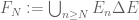
There is an analogue of Exercise 9, which illustrates the extent to which a generated
Exercise 15 (Recursive description of a generated
be the first uncountable ordinal. Define the sets
for every countable ordinal
via transfinite induction as follows:
.
- For each countable successor ordinal
, we define
- For each countable limit ordinal
, we define
.
Show that
.
Remark 5 The first uncountable ordinal
Exercise 16 (This exercise requires familiarity with the theory of cardinals.) Let
(thus
. (Hint: use Exercise 15.) In particular, show that the Borel
.
Conclude that there exist Jordan measurable (and hence Lebesgue measurable) subsets of
Remark 6 Despite this demonstration that not all Lebesgue measurable subsets are Borel measurable, it is remarkably difficult (though not impossible) to exhibit a specific set that is not Borel measurable. Indeed, a large majority of the explicitly constructible sets that one actually encounters in practice tend to be Borel measurable, and one can view the property of Borel measurability intuitively as a kind of “constructibility” property. (Indeed, as a very crude first approximation, one can view the Borel measurable sets as those sets of “countable descriptive complexity”; in contrast, sets of finite descriptive complexity tend to be Jordan measurable (assuming they are bounded, of course).
Exercise 17 Let
be Borel measurable subsets of
respectively. Show that
is a Borel measurable subset of
. (Hint: first establish this in the case when
is a box, by using Remark 4. To obtain the general case, apply Remark 4 yet again.)
The above exercise has a partial converse:
Exercise 18 Let
- Show that for any
, the slice
is a Borel measurable subset of
. Similarly, show that for every
, the slice
is a Borel measurable subset of
.
- Give a counterexample to show that this claim is not true if “Borel” is replaced with “Lebesgue” throughout. (Hint: the Cartesian product of any set with a point is a null set, even if the first set was not measurable.)
Exercise 19 Show that the Lebesgue
— 3. Countably additive measures and measure spaces —
Having set out the concept of a
We begin with the finitely additive theory, although this theory is too weak for our purposes and will soon be supplanted by the countably additive theory.
Definition 6 (Finitely additive measure) Let
that obeys the following axioms:
- (Empty set)
.
- (Finite additivity) Whenever
.
Remark 7 The empty set axiom is needed in order to rule out the degenerate situation in which every set (including the empty set) has infinite measure.
Example 8 Lebesgue measure
is a finitely additive measure on the Lebesgue
On the other hand, as we saw in previous notes, Lebesgue outer measure is not finitely additive on the discrete algebra, and Jordan outer measure is not finitely additive on the Lebesgue algebra.
Example 9 (Dirac measure) Let
and
at
, defined by setting
, is finitely additive.
Example 10 (Zero measure) The zero measure
is a finitely additive measure on any Boolean algebra.
Example 11 (Linear combinations of measures) If
are finitely additive measures on
is also a finitely additive measure, as is
for any
. Thus, for instance, the sum of Lebesgue measure and a Dirac measure is also a finitely additive measure on the Lebesgue algebra (or on any of its sub-algebras).
Example 12 (Restriction of a measure) If
of
whenever
(i.e. if
), is also a finitely additive meaure.
Example 13 (Counting measure) If
defined by setting
to be the cardinality of
if
As with our definition of Boolean algebras and
Exercise 20 Let
- (Monotonicity) If
, then
.
- (Finite additivity) If
is a natural number, and
are
.
- (Finite sub-additivity) If
.
- (Inclusion-exclusion for two sets) If
.
(Caution: remember that the cancellation law
does not hold in
if
is infinite, and so the use of cancellation (or subtraction) should be avoided if possible.)
One can characterise measures completely for any finite algebra:
Exercise 21 Let
of non-empty atoms. Show that for every finitely additive measure
such that
Equivalently, if
is a point in
for each
, then
Furthermore, show that the
are uniquely determined by


This is about the limit of what one can say about finitely additive measures at this level of generality. We now specialise to the countably additive measures on
Definition 7 (Countably additive measure) Let
be a measurable space. An (unsigned) countably additive measure
- (Empty set)
- (Countable additivity) Whenever
are a countable sequence of disjoint measurable sets, then
.
A triplet
, where
Note the distinction between a measure space and a measurable space. The latter has the capability to be equipped with a measure, but the former is actually equipped with a measure.
Example 14 Lebesgue measure is a countably additive measure on the Lebesgue
Example 15 The Dirac measures from Exercise 9 are countably additive, as is counting measure.
Example 16 Any restriction of a countably additive measure to a measurable subspace is again countably additive.
Exercise 22 (Countable combinations of measures) Let
- If
is also countably additive.
- If
are a sequence of countably additive measures on
is also a countably additive measure.
Note that countable additivity measures are necessarily finitely additive (by padding out a finite union into a countable union using the empty set), and so countably additive measures inherit all the properties of finitely additive properties, such as monotonicity and finite subadditivity. But one also has additional properties:
Exercise 23 Let
be a measure space.
- (Countable subadditivity) If
are
.
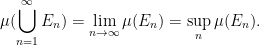
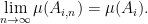
- (Upwards monotone convergence) If
are
- (Downwards monotone convergence) If
are
for at least one
Show that the downward monotone convergence claim can fail if the hypothesis that

Exercise 24 (Dominated convergence for sets) Let
be a sequence of
converges pointwise to
.
- Show that
- If there exists a
) that contains all of the
, show that
. (Hint: Apply downward monotonicity to the sets
.)
- Show that the previous part of this exercise can fail if the hypothesis that all the
Exercise 25 Let
for some
, thus
for all


A null set of a measure space ![{({\bf R}^d, {\mathcal L}[{\bf R}^d], m)}](https://s0.wp.com/latex.php?latex=%7B%28%7B%5Cbf+R%7D%5Ed%2C+%7B%5Cmathcal+L%7D%5B%7B%5Cbf+R%7D%5Ed%5D%2C+m%29%7D&bg=ffffff&fg=000000&s=0&c=20201002)
![{({\bf R}^d, {\mathcal B}[{\bf R}^d], m)}](https://s0.wp.com/latex.php?latex=%7B%28%7B%5Cbf+R%7D%5Ed%2C+%7B%5Cmathcal+B%7D%5B%7B%5Cbf+R%7D%5Ed%5D%2C+m%29%7D&bg=ffffff&fg=000000&s=0&c=20201002)
Completion is a convenient property to have in some cases, particularly when dealing with properties that hold almost everywhere. Fortunately, it is fairly easy to modify any measure space to be complete:
Exercise 26 (Completion) Let
, known as the completion of
consists precisely of those sets that differ from a
Exercise 27 Show that the Lebesgue measure space
— 4. Measurable functions, and integration on a measure space —
Now we are ready to define integration on measure spaces. We first need the notion of a measurable function, which is analogous to that of a continuous function in topology. Recall that a function 


Definition 8 Let
or
be an unsigned or complex-valued function. We say that
is measurable if
of
.
From Lemma 7 of Notes 2, we see that this generalises the notion of a Lebesgue measurable function.
Exercise 28 Let
- Show that a function
are
- Show that an indicator function
- Show that a function
is
- Show that a function
- Show that a function
is measurable if and only if the magnitudes
,
of its positive and negative parts are measurable.
- If
are a sequence of measurable functions that converge pointwise to a limit
- If
is continuous, show that
is measurable. Obtain the same claim if
- Show that the sum or product of two measurable functions in
Remark 8 One can also view measurable functions in a more category theoretic fashion. Define measurable morphism or measurable map
to be a function
-measurable set
is a measurable morphism from
to
with itself repeatedly); but it will not play a major role in this course.
Measurable functions are particularly easy to describe on atomic spaces:
Exercise 29 Let
for some partition
for some constants
in

Exercise 30 (Egorov’s theorem) Let
), and let
be a sequence of measurable functions that converge pointwise almost everywhere to a limit
. Show that there exists a measurable set
such that
converges uniformly to
In Notes 2 we defined first an simple integral, then an unsigned integral, and then finally an absolutely convergent integral. We perform the same three stages here. We begin with the simple integral in the case when the
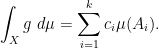
Definition 9 (Simple integral) Let
. If
for some
. We then define the simple integral
of
Note that, thanks to Exercise 3, the precise decomposition into atoms does not affect the definition of the simple integral.


One could also define a simple integral for absolutely convergent complex-valued functions on a measurable space with a finite
With this definition, it is clear that one has the monotonicity property

whenever 

and

for unsigned measurable 
Exercise 31 (Simple integral unaffected by refinements) Let
be a refinement of
agrees with
be measurable. Show that
This allows one to extend the simple integral to simple functions:
Definition 10 (Integral of simple functions) An (unsigned) simple function
. Note that such a function is then automatically measurable with respect to at least one finite sub-
of
where
is the restriction of
Note that there could be multiple finite 


From this we can deduce the following properties of the simple integral. As with the Lebesgue theory, we say that a property 
Exercise 32 (Basic properties of the simple integral) Let
be simple functions.
- (Monotonicity) If
.
- (Compatibility with measure) For every
.
- (Homogeneity) For every
.
- (Finite additivity)
.
- (Insensitivity to refinement) If
is a refinement of
.
- (Almost everywhere equivalence) If
for
.
- (Finiteness)
if and only if
- (Vanishing)
if and only if
Exercise 33 (Inclusion-exclusion principle) Let
be
(Hint: Compute
in two different ways.)

Remark 9 The simple integral could also be defined on finitely additive measure spaces, rather than countably additive ones, and all the above properties would still apply. However, on a finitely additive measure space one would have difficulty extending the integral beyond simple functions, as we will now do.
From the simple integral, we can now define the unsigned integral, similarly to what was done for the unsigned Lebesgue integral in Notes 2:
Definition 11 Let
of

Clearly, this definition generalises the corresponding definition in Definition 10 of Notes 2. Indeed, if ![{f: {\bf R}^d \rightarrow [0,+\infty]}](https://s0.wp.com/latex.php?latex=%7Bf%3A+%7B%5Cbf+R%7D%5Ed+%5Crightarrow+%5B0%2C%2B%5Cinfty%5D%7D&bg=ffffff&fg=000000&s=0&c=20201002)
We record some easy properties of this integral:
Exercise 34 (Easy properties of the unsigned integral) Let
be measurable.
- (Almost everywhere equivalence) If

- (Monotonicity) If
.
- (Homogeneity) We have
for every
- (Superadditivity) We have
.
- (Compatibility with the simple integral) If
.
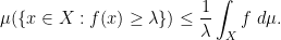
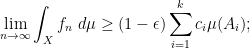
- (Markov’s inequality) For any
, one has
In particular, if
, then the sets
have finite measure for each
.
- (Finiteness) If
is finite for
- (Vanishing) If
, then
- (Horizontal truncation) We have
.
- (Vertical truncation) If
- (Restriction) If
, where
is the restriction of
was defined in Example 12. We will often abbreviate
(by slight abuse of notation) as
.
As before, one of the key properties of this integral is its additivity:
Theorem 12 Let
Proof: In view of super-additivity, it suffices to establish the sub-additivity property

We establish this in stages. We first deal with the case when 


and

Since 

hence by Exercise 34 and the properties of the simple integral,


From (1) we conclude that

Letting 

Now we continue to assume that

Since 

Taking limits as 
Finally, we no longer assume that 


From the previous case, we have

Letting

Exercise 35 (Linearity in
- Show that
for every
- If
are a sequence of measures on
Exercise 36 (Change of variables formula) Let
be a measurable morphism (as defined in Remark 8) from
of
by the formula
.
- Show that
is a measure on
is a measure space.
- If
is measurable, show that
.
(Hint: the quickest proof here is via the monotone convergence theorem below, but it is also possible to prove the exercise without this theorem.)
Exercise 37 Let
be an invertible linear transformation, and let
, where the pushforward
of
Exercise 38 (Sums as integrals) Let
be counting measure (see Exercise 13), and let

Once one has the unsigned integral, one can define the absolutely convergent integral exactly as in the Lebesgue case:
Definition 13 (Absolutely convergent integral) Let
is finite, and use
,
, or
to denote the space of absolutely integrable functions. If
where
where the two integrals on the right are interpreted as real-valued integrals. It is easy to see that the unsigned, real-valued, and complex-valued integrals defined in this manner are compatible on their common domains of definition.

Clearly, this definition generalises the corresponding definition in Definition 13 of Notes 2.
We record some of the key facts about the absolutely convergent integral:
Exercise 39 Let
- Show that
- Show that the integration map
is a complex-linear map from
- Establish the triangle inequality
and the homogeneity property
for all
and
.
- Show that if
are such that
.
- If
, and
, and
. (Hint: it is easy to get one inequality. To get the other inequality, first work in the case when
- Show that if
if and only if
- If
is
and
. As before, by abuse of notation we write
.
— 5. The convergence theorems —
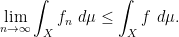
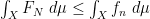
Let ![{f_1, f_2, \ldots: X \rightarrow [0,+\infty]}](https://s0.wp.com/latex.php?latex=%7Bf_1%2C+f_2%2C+%5Cldots%3A+X+%5Crightarrow+%5B0%2C%2B%5Cinfty%5D%7D&bg=ffffff&fg=000000&s=0&c=20201002)

To put it another way: when can we ensure that one can interchange integrals and limits,
There are certainly some cases in which one can safely do this:
Exercise 40 (Uniform convergence on a finite measure space) Suppose that
), and
converges to
However, there are also cases in which one cannot interchange limits and integrals, even when the
Example 17 (Escape to horizontal infinity) Let
. Then
, but
does not converge to
. Somehow, all the mass in the
Example 18 (Escape to width infinity) Let
. Then
Example 19 (Escape to vertical infinity) Let
with Lebesgue measure (restricted from
), and let
. Now, we have finite measure, and
is not converging to
. This time, the mass has escaped vertically, through the increasingly large values of
Remark 10 From the perspective of time-frequency analysis (or perhaps more accurately, space-frequency analysis), these three escapes are analogous (though not quite identical) to escape to spatial infinity, escape to zero frequency, and escape to infinite frequency respectively, thus describing the three different ways in which phase space fails to be compact (if one excises the zero frequency as being singular).
However, once one shuts down these avenues of escape to infinity, it turns out that one can recover convergence of the integral. There are two major ways to accomplish this. One is to enforce monotonicity, which prevents each 
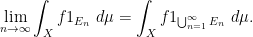
Theorem 14 (Monotone convergence theorem) Let
be a monotone non-decreasing sequence of unsigned measurable functions on

Note that in the special case when each 
Proof: Write 
It remains to establish the reverse inequality
By definition, it suffices to show that

whenever 

for some 
Let 

for all 

then the 

On the other hand, observe the pointwise bound

for any

Taking limits as
sending
Remark 11 It is easy to see that the result still holds if the monotonicity
only holds almost everywhere rather than everywhere.
This has a number of important corollaries. Firstly, we can generalise (part of) Tonelli’s theorem for exchanging sums (see Theorem 2 of Notes 1):
Corollary 15 (Tonelli’s theorem for sums and integrals) Let
be a sequence of unsigned measurable functions. Then one has
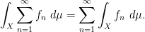
Proof: Apply the monotone convergence theorem to the partial sums 
Exercise 41 Give an example to show that this corollary can fail if the
is absolutely convergent for each
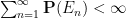
Exercise 42 (Borel-Cantelli lemma) Let
be a measure space, and let
be a sequence of
. Show that almost every
is finite for almost every
Exercise 43
- Give an alternate proof of the Borel-Cantelli lemma (Exercise 42) that does not go through any of the convergence theorems, but instead exploits the more basic properties of measure from Exercise 23.
- Give a counterexample that shows that the Borel-Cantelli lemma can fail if the condition
.
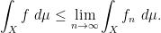
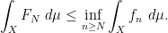
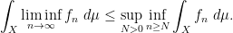
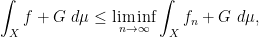
Secondly, when one does not have monotonicity, one can at least obtain an important inequality, known as Fatou’s lemma:
Corollary 16 (Fatou’s lemma) Let
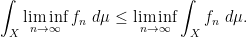
Proof: Write 


By definition of lim inf, we have 

Hence we have
The claim then follows by another appeal to the definition of lim inf.
Remark 12 Informally, Fatou’s lemma tells us that when taking the pointwise limit of unsigned functions
). While this lemma was stated only for pointwise limits, the same general principle (that mass can be destroyed, but not created, by the process of taking limits) tends to hold for other “weak” notions of convergence. We will see some instances of this in 245B.
Finally, we give the other major way to shut down loss of mass via escape to infinity, which is to dominate all of the functions involved by an absolutely convergent one. This result is known as the dominated convergence theorem:
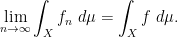
Theorem 17 (Dominated convergence theorem) Let
be a sequence of measurable functions that converge pointwise
such that
are pointwise
for each
From the moving bump examples we see that this statement fails if there is no absolutely integrable dominating function
Proof: By modifying 

By taking real and imaginary parts we may assume without loss of generality that 

If we apply Fatou’s lemma to the unsigned functions 
which on subtracting the finite quantity 

Similarly, if we apply that lemma to the unsigned functions 

negating this inequality and then cancelling

The claim then follows by combining these inequalities.
Remark 13 We deduced the dominated convergence theorem from Fatou’s lemma, and Fatou’s lemma from the monotone convergence theorem. However, one can obtain these theorems in a different order, depending on one’s taste, as they are so closely related. For instance, in Stein-Shakarchi, the logic is somewhat different; one first obtains the slightly simpler bounded convergence theorem, which is the dominated convergence theorem under the assumption that the functions are uniformly bounded and all supported on a single set of finite measure, and then uses that to deduce Fatou’s lemma, which in turn is used to deduce the monotone convergence theorem; and then the horizontal and vertical truncation properties are used to extend the bounded convergence theorem to the dominated convergence theorem. It is instructive to view a couple different derivations of these key theorems to get more of an intuitive understanding as to how they work.
Exercise 44 Under the hypotheses of the dominated convergence theorem, establish also that
as
Exercise 45 (Almost dominated convergence) Let
such that the
, and that
as
Exercise 46 (Defect version of Fatou’s lemma) Let
as
.) Informally, this tells us that the gap between the left and right hand sides of Fatou’s lemma can be measured by the quantity
.

Exercise 47 Let
be measurable. Show that the function
defined by the formula
is a measure. (We will study such measures in greater detail in 245B.)

The monotone convergence theorem is, in some sense, a defining property of the unsigned integral, as the following exercise illustrates.
Exercise 48 (Characterisation of the unsigned integral) Let
be a map from the space
of unsigned measurable functions
- (Homogeneity) For every
and
.
- (Finite additivity) For every
, one has
.
- (Monotone convergence) If
.
Then there exists a unique measure
for all
for all
Exercise 49 Let
and lower integral
agree. Show that


We will continue to see the monotone convergence theorem, Fatou’s lemma, and the dominated convergence theorem make an appearance throughout the rest of this course sequence.
— 6. Probability spaces (optional) —
We now pause to isolate a special type of measure space, namely an probability space. As the name suggests, these spaces are of fundamental importance in the foundations of probability, although it should be emphasised that probability theory should not be viewed as the study of probability spaces, as these are merely models for the true objects of study of that theory, namely the behaviour of random events and random variables. (See this post for further discussion of this point.) This course will not be focused on applications to probability theory, but other courses (such as the Math 275 sequence at UCLA) will certainly be taking several results from measure theory (e.g. the Borel-Cantelli lemma, Exercise 42) and transferring them to a probabilistic context in order to apply them to problems of interest in probability theory.
Definition 18 (Probability space) A probability space is a measure space
of total measure
:
. The measure
is known as a probability measure.
Note the change of notation: whereas measure spaces are traditionally denoted by symbols such as 
- The space
that a random system could be in.
- The
- The measure
of an event is known as the probability of that event.
The various axioms of a probability space then formalise the foundational axioms of probability, as set out by Kolmogorov.
Example 20 (Normalised measure) Given any measure space
, the space
is a probability space. For instance, if
and the counting measure
is a probability measure (known as the (discrete) uniform probability measure on
is a probability space. In probability theory, this probability spaces models the act of drawing an element of the discrete set
Similarly, if
is a Lebesgue measurable set of positive finite Lebesgue measure,
, then
is a probability space. The probability measure
is known as the (continuous) uniform probability measure on
Example 21 (Discrete and continuous probability measures) If
are a collection of real numbers in
, then the probability measure
, or in other words
is indeed a probability measure, and
is a probability space. The function
is known as the (discrete) probability distribution of the state variable
.
Similarly, if
is a Lebesgue measurable function on
, then
is a probability space, where
is the measure
The function


Exercise 50 (No translation-invariant random integer) Show that there is no probability measure
with the discrete
with the translation-invariance property
for every event
and every integer
Exercise 51 (No translation-invariant random real) Show that there is no probability measure
with the translation-invariance property
for every event
and every real
Many concepts in measure theory are of importance in probability theory, although the terminology is changed to reflect the different perspective on the subject. For instance, the notion of a property holding almost everywhere is now replaced with that of a property holding almost surely. A measurable function is now referred to as a random variable and is often denoted by symbols such as 

In later notes, when we develop the machinery of product measures and other tools to construct measures, we will see some more interesting examples of probability spaces, which would correspond in probability theory to random processes that are generated by an infinite number of independent random sources.
The following exercise will be moved to a more suitable location in the published version of the notes, but is here currently so as not to disrupt the exercise numbering.
Exercise 52 (Approximation by an algebra) Let
be a Boolean algebra on
.
- If
and
such that
.
- More generally, if
for some
with
for all

120 comments
Comments feed for this article
25 July, 2013 at 4:21 am
Luqing Ye
A remark to Theorem 17 (Dominated convergence theorem):
I proved the dominated convergence theorem using Egorove’s theorem together with Exercise 40 (Uniform convergence on a finite measure space) when I was walking outside home.
I don’t use Fatou’s lemma…..BTW,I think Fatou’s lemma is a naive and easy stuff,so I will be comfortable that I don’t use this lemma….
25 July, 2013 at 9:16 pm
Luqing Ye
Dear Prof.Tao,
In the proof of Theorem 17 (Dominated convergence theorem),I think the last inequality
should be
25 July, 2013 at 9:25 pm
Luqing Ye
I am wrong again……Maybe next time I shouldn’t put any comment until I think 10 times.
26 July, 2013 at 6:50 am
A proof of Fatou’s lemma « Asymptote
[…] In this post I give a proof of Fatou’s lemma which is the Corollary 16 of Terence Tao’s post 245A, Notes 3: Integration on abstract measure spaces, and the convergence theorems. […]
28 July, 2013 at 7:03 am
Luqing Ye
Dear Prof.Tao,
Could you please give me some hints on how the condition “Suppose that is complete, which means that every sub-null set is a null set.” is used in Exercise 49?
I have a bit doubt on my ability to give a correct proof because I proved Exercise 49 without using this condition……
28 July, 2013 at 8:38 am
Terence Tao
If is an indicator function of a sub-null set, what are the upper and lower integrals of
  ?
?
28 July, 2013 at 8:38 pm
Luqing Ye
If is an indicator function of an unmeasurable sub-null set,it seems that the upper and lower integrals of
  does not exist.
Dear Prof.Tao,
Thank you for your hint.Now I understand that I made a skip in my proof,I thought that according to Littlewood’s principle,I can ignore the subnull set and null set but actually I should not because if I ignore the unmeasurable subnull set,then I will get an unmeasurable monster.
The reason that I proved this exercise wrongly is that I used wrong intuition.I carry my intuition in Lebesgue measure into this general measure space setting,which result in my fault.More precisely,it seems that Littlewood’s three principle should only work in complete measure space,otherwise I will get a monster……
4 July, 2016 at 6:15 pm
Sunting
i think the important aspect is that if X is not complete, then if fn(measurable) converges to f, a.e., we could not say that f is measurable. if it is complete, then f is measurable.if f is an indicator function of subnull set, then upper and lower integrals both are zero, so they agree, but it seems that in this case f is not measurable.
1 September, 2014 at 4:41 pm
Anonymous
Are Borel sigma algebra![{\mathcal B}[{\bf C}]](https://s0.wp.com/latex.php?latex=%7B%5Cmathcal+B%7D%5B%7B%5Cbf+C%7D%5D&bg=ffffff&fg=545454&s=0&c=20201002) and
and ![{\mathcal B}[{\bf R}^2]](https://s0.wp.com/latex.php?latex=%7B%5Cmathcal+B%7D%5B%7B%5Cbf+R%7D%5E2%5D&bg=ffffff&fg=545454&s=0&c=20201002) the same? In Folland’s Real Analysis, the author uses
the same? In Folland’s Real Analysis, the author uses ![{\mathcal B}[{\bf C}]={\mathcal B}[{\bf R}^2]](https://s0.wp.com/latex.php?latex=%7B%5Cmathcal+B%7D%5B%7B%5Cbf+C%7D%5D%3D%7B%5Cmathcal+B%7D%5B%7B%5Cbf+R%7D%5E2%5D&bg=ffffff&fg=545454&s=0&c=20201002) to show that a complex function is measurable iff both the real and imaginary parts are measurable.
to show that a complex function is measurable iff both the real and imaginary parts are measurable.
1 September, 2014 at 5:13 pm
Terence Tao
1 September, 2014 at 5:36 pm
Anonymous
When you say “identifying”, do you mean “homeomorphism”? In one has multiplication for
  . But in
  , one only has inner product
  , which is not the same as the previous one. Is it because one discards such structures and considers “topology” only that one can “identify” these two Borel sigma algebra. As I understand from your comment, should one view “=” in the identity above as “homromorphism” (or some sort of “isomorphism”)?
1 September, 2014 at 6:51 pm
Terence Tao
The standard identification between
  and
and  is an isomorphism of sets (otherwise known as a bijection), and is furthermore an isomorphism of topological spaces (otherwise known as a homeomorphism). As you noted, though, it is not an isomorphism of rings or of inner product spaces. (It is an isomorphism of (additive) groups, but this is not particularly relevant for the current discussion.)
19 September, 2014 at 12:56 pm
Anonymous
I don’t follow the “without loss of generality” part of the proof of MCT. Suppose is not finite every where, say,
  and
and  is not of measure zero. How to go on in this situation? How does “vertical truncation” help here (I don’t know what is “truncated” here…)?
19 September, 2014 at 2:20 pm
Terence Tao
If g attains infinite values, replace g with (this is the “vertical truncation” of g at height N) and then let
  .
.
24 May, 2015 at 7:20 am
Alex
Do you have any additional hint on how to prove the dominated convergence theorem for sets? Following the given hint, one takes

 ?
?
and by monotone convergence for sets
How can I prove that
Thank you!
[You don’t need to prove to finish the problem. One just needs an appropriate inequality relating
  with
with  and
and  . -T.]
29 September, 2015 at 9:54 pm
275A, Notes 0: Foundations of probability theory | What's new
[…] begin with the notion of a measurable space. (See also this previous blog post, which covers similar material from the perspective of a real analysis graduate class rather than a […]
2 October, 2015 at 10:11 pm
TECNOLOGÍA » 275A, Notes 0: Foundations of probability theory
[…] begin with the notion of a measurable space. (See also this previous blog post, which covers similar material from the perspective of a real analysis graduate class rather than a […]
3 October, 2015 at 2:58 pm
275A, Notes 1: Integration and expectation | What's new
[…] of the details of this construction will be left to exercises. See also Chapter 1 of Durrett, or these previous blog notes, for a more detailed […]
16 December, 2015 at 4:22 pm
Anonymous
In the proof of MCT, why we need the there? What could fail if we just define
the sets
16 December, 2015 at 4:26 pm
Anonymous
I meant
16 December, 2015 at 4:37 pm
Terence Tao
In this case, the need not increase to
  . (For instance, one could have
  on
on  .)
.)
17 December, 2015 at 10:55 am
Anonymous
The reader is encouraged to see why, in each of the moving bump examples, no such dominating function exists, without appealing to the above theorem (DCT)
To dominate
17 December, 2015 at 12:47 pm
Terence Tao
Graph the functions , and compare against the graph of
  .
.
1 August, 2016 at 7:02 am
Joe Li
Small typo in Exercise 31.![f: {\mathcal B} \rightarrow [0,+\infty]](https://s0.wp.com/latex.php?latex=f%3A+%7B%5Cmathcal+B%7D+%5Crightarrow+%5B0%2C%2B%5Cinfty%5D&bg=ffffff&fg=545454&s=0&c=20201002) should be
should be ![f: X \rightarrow [0,+\infty]](https://s0.wp.com/latex.php?latex=f%3A+X+%5Crightarrow+%5B0%2C%2B%5Cinfty%5D&bg=ffffff&fg=545454&s=0&c=20201002) .
.
[Corrected, thanks – T.]
22 November, 2016 at 7:25 am
coupon_clipper
Sorry for the simple question, but can you give a hint for Exercise 34 part 10 (vertical truncation)? I feel like none of the old tricks from Lebesgue integration work here, and we don’t even know if the union of the have finite measure. Every time I try to write out a proof, I end up trying to switch limits around, which is what I’m trying to prove I can do.
[First try the case when is a simple function, or even an indicator function. -T.]
23 November, 2016 at 2:43 pm
Coupon_clipper
Thanks Terry. Got it now. Have a great Thanksgiving!
12 March, 2017 at 11:08 pm
Ian
Concerning exercise 18, part 1: Is this statement true? How can one prove that if E has measurable projection, then its complement does too? (since projection does not commute with taking complements)
[Exercise 18 concerns slices, not projections. -T]
16 January, 2019 at 10:57 am
245A: Problem solving strategies | What's new
[…] the generating sets; in some cases one can also take balls, cubes, or rectangles); see Remark 4 of Notes 3. One can relax the set of properties required, for instance countable intersections is […]
21 June, 2020 at 12:37 am
Ruijun Lin
I want to ask a question on Exercise 26 about completion. Do we need to just to prove the existence first then find the structure of the completed space? Or first construct one then show it satisfies all the conditions?
[Either approach can work, although the latter is easier in this case -T.]
28 June, 2020 at 4:31 am
Ruijun Lin
Thanks Prof. Tao
28 June, 2020 at 4:41 am
Ruijun Lin
Dear Prof. Tao,
I tried hard but cannot figure out the complete proof of the Exercise 36 about the change of variables formula about the pushforward measure without the monotone convergence theorem. The question (i) is simple and I made it.For (ii) I only know how to show the conclusion holds for simple functions. But for general unsigned functions I failed to work it out. Can you give a proof or offer just some hints for the general case without the monotone convergence theorem?
Thank you very much.
28 June, 2020 at 6:58 am
Ruijun Lin
Yes, I’m very eager to know the proof of this problem without the monotone convergence theorem to maintain the fluency of the book.
29 June, 2020 at 10:35 pm
Leo Sera
Hi Ruijun. Looks like someone asked the same question you did here and it already has an answer. https://math.stackexchange.com/questions/3738431/proof-of-the-change-of-variables-formula-without-using-the-monotone-convergence/3738505#3738505
30 June, 2020 at 1:07 am
Ruijun Lin
(Laughter) The question there is also asked by me.
30 June, 2020 at 1:09 am
Ruijun Lin
Maybe there is an answer and I will check it.
30 June, 2020 at 3:21 am
Ruijun Lin
His answer is wrong, I think.
30 June, 2020 at 7:42 pm
Leo Sera
Oh! I just read it I didn’t see the error but looks like it has a couple of edits. Maybe the error you caught has been fixed.
4 January, 2021 at 12:46 pm
Anonymous
If one wants to develop an integration theory for functions defined on manifolds, does one need to (eventually) use coordinate charts? Or does the nature of “abstract” measure spaces allow one to define Lebesgue integrals in an intrinsic way?
4 January, 2021 at 7:31 pm
Terence Tao
There is no canonical measure that one can intrinsically assign to an smooth abstract manifold (pushing forward Lebesgue measure from a coordinate chart is a chart-dependent construction). But if one has an additional structure, such as a Riemannian metric, a symplectic form, Kahler measure, a transitive group action by an amenable group, or an immersion into Euclidean space, one can often create such a canonical measure (Riemannian volume measure, Liouville measure, Haar measure, induced Lebesgue measure, etc.).
16 March, 2022 at 7:06 am
Anonymous
In the case of the counting measure, one has in Exercise 38 the integral is actually a sum. Does one has a simple formula for when
when  is the Dirac delta measure, say
  for some fixed
  ?
?
16 March, 2022 at 9:57 am
Terence Tao
Yes, this is .
.
22 May, 2022 at 10:08 am
Anonymous
Dear Professor Tao: sets has most
  atoms, first showing by induction that
  sets partition the space into at most
  disjoint regions?
For exercise 8, is it ideal to prove it by showing that the Boolean algebra generated by
[Sure, that works – T.]
6 June, 2022 at 7:39 am
YiLi
Dear Professor Tao: For exercise 35 change of variable formula, I was confused with the version of change of variable formula in the context of calculus, where needs the transformation being at least $C^1$ diffeomorphism? why only needs morphism not isomorphism here?
11 June, 2022 at 3:21 pm
Terence Tao
The measure-theory perspective allows one to split the change of variables formula into two parts and clarifies exactly where a hypothesis of diffeomorphism is helpful. The first, which is purely measure-theoretic and requires no assumption of diffeomorphism, is Exercise 35 here. The second, which is not part of this notes, is that the pushforward of Lebesgue measure under a
  diffeomorphism
  is given by
  . Thus one can push forward a measure (or pull back an integral) by arbitrary measurable maps, but one is not guaranteed to have a nice formula for this change of variables unless one has a diffeomorphism structure (or other nice property of the map).
12 June, 2022 at 5:27 am
YiLi
I got it thank you, the pull back measure has some set theory beneficial, for example in the construction of the measure preserving map in the Ergodic Theory.
6 February, 2023 at 3:33 pm
Anonymous
Dear professor Tao:
For exercise $23$, What would be an example of such a sequence of sets if the hypothesis that ${\mu(E_n)<\infty}$ for at least one $n$ is dropped? I find it hard to utilize the middle third Cantor set example in this case.
[Hint: experiment with half-infinite intervals in the real line. -T]
12 February, 2023 at 4:10 pm
sam
Dear professor Tao: is an algebra on
  for each n, and then
  , in order to use part (1) on the finite measure space
  . (Here the intersection of an algebra with a set is the collection of the intersection of that set with the members of the algebra). Is this the way the solution is intended? What else can one approaches the problem?
For part (2) of exercise 28(in the textbook), I think one first needs to show that
23 February, 2023 at 4:44 pm
Anonymous
Dear professor Tao: with
with  in exercise 21 of note 1?
For exercise 37, can we prove it by simply replace
[Yes – T.]
27 February, 2023 at 3:07 pm
Anonymous
Dear professor Tao: of Exercise $ latex 39$, it looks like the fact that the integral of
  being insensitive to refinement follows from the same property of the real-valued
  , which follows from that of the unsigned
  , which then follows from that of the simple $f$. Why then do we need to approximate $f$ as the hint suggested?
For
[This also works – T.]