
As in previous posts, we use the following asymptotic notation: 


The purpose of this post is to collect together all the various refinements to the second half of Zhang’s paper that have been obtained as part of the polymath8 project and present them as a coherent argument (though not fully self-contained, as we will need some lemmas from previous posts).
In order to state the main result, we need to recall some definitions.
Definition 1 (Singleton congruence class system) Let
, and let
denote the square-free numbers whose prime factors lie in
. A singleton congruence class system on
of primitive residue classes
for each
, obeying the Chinese remainder theorem property
whenever
are coprime. We say that such a system
has controlled multiplicity if the
for any fixed
and any congruence class
with
. Here
is the divisor function.


Next we need a relaxation of the concept of 
Definition 2 (Dense divisibility) Let
. A positive integer
, there exists a factor of
. We let
denote the set of
Now we present a strengthened version ![{MPZ'[\varpi,\delta]}](https://s0.wp.com/latex.php?latex=%7BMPZ%27%5B%5Cvarpi%2C%5Cdelta%5D%7D&bg=ffffff&fg=000000&s=0&c=20201002)
![{MPZ[\varpi,\delta]}](https://s0.wp.com/latex.php?latex=%7BMPZ%5B%5Cvarpi%2C%5Cdelta%5D%7D&bg=ffffff&fg=000000&s=0&c=20201002)


Conjecture 3 (
be a congruence class system with controlled multiplicity. Then
for any fixed
, where
is the von Mangoldt function.
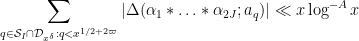
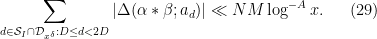
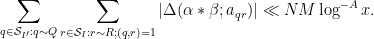
![\displaystyle \sum_{q \in {\mathcal S}_I \cap {\mathcal D}_{x^\delta}: q< x^{1/2+2\varpi}} |\Delta(\Lambda 1_{[x,2x]}; a_q)| \ll x \log^{-A} x \ \ \ \ \ (3)](https://s0.wp.com/latex.php?latex=%5Cdisplaystyle++%5Csum_%7Bq+%5Cin+%7B%5Cmathcal+S%7D_I+%5Ccap+%7B%5Cmathcal+D%7D_%7Bx%5E%5Cdelta%7D%3A+q%3C+x%5E%7B1%2F2%2B2%5Cvarpi%7D%7D+%7C%5CDelta%28%5CLambda+1_%7B%5Bx%2C2x%5D%7D%3B+a_q%29%7C+%5Cll+x+%5Clog%5E%7B-A%7D+x+%5C+%5C+%5C+%5C+%5C+%283%29&bg=ffffff&fg=000000&s=0&c=20201002)
The difference between this conjecture and the weaker conjecture 
![{[1,x^\delta]}](https://s0.wp.com/latex.php?latex=%7B%5B1%2Cx%5E%5Cdelta%5D%7D&bg=ffffff&fg=000000&s=0&c=20201002)
![{DHL[k_0,2]}](https://s0.wp.com/latex.php?latex=%7BDHL%5Bk_0%2C2%5D%7D&bg=ffffff&fg=000000&s=0&c=20201002)
The main result we will establish is
 with
with 
This improves upon previous constraints of 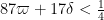


— 1. Reduction to Type I/II and Type III estimates —
Following Zhang, we can perform a combinatorial reduction to reduce Theorem 4 to two sub-estimates. To state this properly we need some more notation. We need a large fixed constant 
Definition 5 (Coefficient sequences) A coefficient sequence is a finitely supported sequence
that obeys the bounds
for all
.
- (i) If
is a coefficient sequence and
is a primitive residue class, the (signed) discrepancy
of
- (ii) A coefficient sequence
for some
if it is supported on an interval of the form
.
- (iii) A coefficient sequence
for any
, any fixed
, and any primitive residue class
- (iv) A coefficient sequence
for some smooth function
supported on
obeying the derivative bounds
for all fixed
(note that the implied constant in the
notation may depend on
).


We can now state the two subestimates needed. The first controls sums of Type I or Type II:
Theorem 6 (Type I/II estimate) Let
be fixed quantities such that
and let
be coefficient sequences at scales
respectively with
with
obeying a Siegel-Walfisz theorem. Then for any


This improves upon Theorem 16 in this previous post, in which the modulus was required to be 

The second subestimate controls sums of Type III:
Theorem 7 (Type III estimate) Let
be fixed quantities. Let
be scales obeying the relations
and
for some fixed
. Let
be coefficient sequences at scales
respectively, with
smooth. Then for any
for any fixed


This improves upon Theorem 17 in this previous post, in which the modulus was required to be 
Let us now recall the combinatorial argument (from this previous post) that allows one to deduce Theorem 4 from Theorems 6 and 7. As in Section 3 of this previous post, we let 

where 
- (i) Each
is a coefficient sequence at scale
. More generally the convolution
of the
is a coefficient sequence at scale
.
- (ii) If
for some fixed
- (iii) If
for some fixed
for some fixed
- (iv)
.
We can write 


to be chosen later and conclude one of the following:
- (Type 0) There is a
.
- (Type I/II) There is a partition
such that
- (Type III) There exist distinct
with
and
.
In the Type 0 case, we can write 


provided that we can verify the hypotheses (15), (16), (17), which will follow if we have

and

and

Since 

and
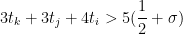
so we will be done if we can find 

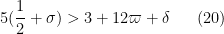

The condition (20) is a consequence of (19) and can thus be omitted.
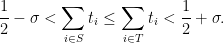
We rewrite all of the constraints in terms of upper and lower bounds on

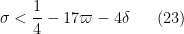
while the lower bounds take the form

Clearly (22) is implied by (23), and (26) is implied by (27); restricting to the case 
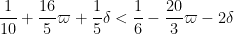
but this rearranges to (4).
It remains to establish Theorem 6 and Theorem 7.
— 2. Type I/II analysis —
We begin the proof of Theorem 6, closely following the arguments from Section 5 of this previous post. We can restrict

for some sufficiently slowly decaying 
for any 


be an exponent to be optimised later (in the Type I case, it will be infinitesimally close to zero, while in the Type II case, it will be infinitesimally larger than 
By Lemma 11 of this previous post, we know that for all 
![{[D,2D]}](https://s0.wp.com/latex.php?latex=%7B%5BD%2C2D%5D%7D&bg=ffffff&fg=000000&s=0&c=20201002)
where

Specifically, the number of exceptions in the interval 

with 

and
By dyadic decomposition, it thus sufices to show that
for any fixed 


Fix 


We now split the discrepancy

as the sum of the subdiscrepancies

and

In Section 5 of this previous post, it was established that


As in the previous notes, we will not take advantage of the 


for each individual 

whenever 
By duality and Cauchy-Schwarz exactly as in Section 5 of the previous post, it suffices to show that


for any fixed 


where 


As in the previous notes, we can dispose of the case when
which we file away for later. (There was also the condition 


It remains to verify (40). Observe that 


note that these inverses in the various rings 


We may write 


for some 


Applying completion of sums (Section 2 from the previous post), we reduce to showing that

for a sufficiently small fixed

 is the phase
and we have dropped all hypotheses on 

We now split into two cases, one which works when 

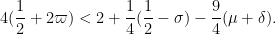
Theorem 8 (Type I case) If the inequalities
hold for some fixed
, then (43) holds for a sufficiently small fixed


The hypotheses (46), (47), (48) improve upon Theorem 13 from this previous post, which had instead the more strict condition

In practice the condition (47) is dominant.
Now we give the Type II estimate:
Theorem 9 (Type II case) If the inequality
holds, then (43) holds for a sufficiently small fixed

This result improves upon Theorem 14 from this previous post which had the stronger condition

In practice, (50) will not hold with the original value of 

Assuming these theorems, let us now conclude the proof of Theorem 6. First suppose we are in the “Type I” regime when (49) holds for some fixed

which means that the condition (39) is now weaker than (30) (for 
Now suppose instead that we are in the “Type II” regime where (49) fails for some small

From this we see that we may replace 

which is satisfied for 
In the next two sections we establish Theorem 8 and Theorem 9.
— 3. The Type I sum —
We now prove Theorem 8. It suffices to show that

for any bounded real coefficients 

for any 
To prove (51), we isolate the diagonal case 


but this follows from (33), (49) for
Now we treat the non-diagonal case 
Lemma 10 In the non-diagonal case

Proof: From (45) we may of course assume that

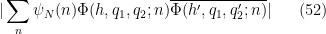
Arguing as in Section 6 of this previous post, we may write the left-hand side of (52) as
where 
![{d_2 := [q_2, q'_2]}](https://s0.wp.com/latex.php?latex=%7Bd_2+%3A%3D+%5Bq_2%2C+q%27_2%5D%7D&bg=ffffff&fg=000000&s=0&c=20201002)


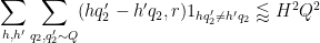
Now for the new input that was not present in the previous Type I analysis. Applying Proposition 5(iii) from this previous post, and noting that 

Since 


the claim follows.

Note from the divisor bound that for each choice of 


and thus also if 


so to conclude (51) we need to show that

and

and

Using (44), (13) we can rewrite these criteria as

and

and
respectively. Applying (33), (32), it suffices to verify that

and

and
respectively. These rearrange to (46), (47), (48) respectively, and the claim follows.
— 4. The Type II sum —
We now prove Theorem 9. Arguing as in Section 7 of this previous post, it suffices to show that


As in the previous post, the diagonal case 
but this is automatic from (32) and (30) if
We have the following analogue of Lemma 10:
Lemma 11 In the off-diagonal case
, we have


This is an improved version of the estimate (48) from this previous post in which several inefficiencies in the second term on the right-hand side have been removed.
Proof: From (45) we may assume

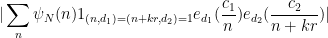
and by the arguments from the previous post we may rewrite the left-hand side of (55) as

where
![\displaystyle d_1 := [q_1,q'_1]r; \quad d_2 := [q_2,q'_2]](https://s0.wp.com/latex.php?latex=%5Cdisplaystyle++d_1+%3A%3D+%5Bq_1%2Cq%27_1%5Dr%3B+%5Cquad+d_2+%3A%3D+%5Bq_2%2Cq%27_2%5D&bg=ffffff&fg=000000&s=0&c=20201002)
and

By Proposition 5(ii) of this previous post, we may the bound this quantity by
![\displaystyle \lessapprox [d_1,d_2]^{1/2} + \frac{N}{d_1 d_2} (d_1,d_2)^2 (c_1,d'_1) (c_2,d'_2)](https://s0.wp.com/latex.php?latex=%5Cdisplaystyle++%5Clessapprox+%5Bd_1%2Cd_2%5D%5E%7B1%2F2%7D+%2B+%5Cfrac%7BN%7D%7Bd_1+d_2%7D+%28d_1%2Cd_2%29%5E2+%28c_1%2Cd%27_1%29+%28c_2%2Cd%27_2%29&bg=ffffff&fg=000000&s=0&c=20201002)
where 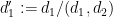


since 

Arguing as in the previous section we have
and so the off-diagonal contribution to (54) is
To conclude (54) we thus need to show that

and

Using (44), (13) we can rewrite these criteria as

and
respectively. Applying (33), (32), it suffices to verify that

and

which can be rearranged as

and

respectively, and thus both follow from (50).
— 5. The Type III estimate —
Now we prove Theorem 7. Our arguments will closely track those of Section 2 of this previous post, except that we will carry the
Let 
for all 


Fix

for some 

plus the error terms

and a tiny error

for any fixed


it will suffice to prove the following claim:
Proposition 12 Let
be fixed, and let
be such that
for some fixed
, and let
be smooth coefficient sequences at scale
respectively. Then
if


Let us now see why the above proposition implies (57). To prove (57), we may of course assume 
for any function 

which we expand as
In order to apply Proposition 12 we need to modify the 


for any function 


where


We may discard those values of 


which by the divisor bound is 
It remains to prove Proposition 12. Note from (58), (59) one has

Expanding out the 


The next step is Weyl differencing. We will need a step size 

we will make the hypothesis that

and save this condition to be verified later.
By shifting 


By the triangle inequality, it thus suffices to show that
Next, we combine the 

for any fixed 


where 


Thus we can estimate the left-hand side of (69) by

where
Here we have bounded 

We will eliminate the 


and thus

Note that 


From the divisor bound, we see that for each fixed 


From this, (70), and Cauchy-Schwarz, we see that to prove (69) it will suffice to show that

We square out (71) as

If we shift 


Next we perform another completion of sums, this time in the 


by

(the prime is there to distinguish this quantity from
Making the change of variables 


where
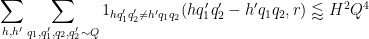
Applying the Bombieri-Birch bound (Theorem 4 from this previous post), and recalling that


We may cross multiply and write

By the divisor bound, for each choice of 


We now choose

for some
Lemma 13 If
, then we have

Proof: We first consider the contribution of the diagonal case 
The 

For the non-diagonal case 

since 

From this lemma, we see that we are done if we can find

as well as the previously recorded condition (68). We can split the condition (73) into three subconditions:


Substituting the definitions (67), (72) of 
while the other three conditions rearrange to


and

We can replace the first two constraints by the stronger constraint

We combine these constraints as

where


and from (62), (63) we have 

since ![{[x^{-\delta} R, R]}](https://s0.wp.com/latex.php?latex=%7B%5Bx%5E%7B-%5Cdelta%7D+R%2C+R%5D%7D&bg=ffffff&fg=000000&s=0&c=20201002)


It remains to establish 


86 comments
Comments feed for this article
23 June, 2013 at 11:12 pm
Terence Tao
Once again recording the latest critical numerology. If we ignore and infinitesimals, then we have
and the critical term in the Heath-Brown identity is now of the form
where are smooth and at scale
  and
and  is at scale
  with
with
thus are at scale
  , and
, and  is at scale
  . We are still a little bit above the combinatorial constraint
  but we will be bumping against that pretty soonish.
This critical case is on the Type I / Type III border; both arguments apply to this case, and improving either of them at this choice of parameters should lead to an improvement in the final value of . (On the other hand, the Type II analysis is not critical here, and we do not urgently need to improve that analysis further for the time being). With the Type I analysis, we may group
  and
and  as
as  and
and  respectively, and the parameter scales are
In Lemma 10, it is the middle term which dominates slightly, suggesting that there is a little bit of gain to be had by refactoring to reduce
  and increase
  .
.
Meanwhile, in the Type III analysis, the numerology is
In Lemma 13 the last two terms on the RHS are equal and dominant.
30 June, 2013 at 11:01 pm
v08ltu
I am confused, in (49) you give a constraint for Type II that has (in particular), but then you take
  ? Is
? Is  allowed to be negative?
30 June, 2013 at 11:04 pm
v08ltu
OK, I guess you explain it right below (49), that “ ” is really not such, but a different thing that is really only
  .
.
23 June, 2013 at 11:50 pm
v08ltu
I think reshufffling the divisors to reduce slightly, would make
  dominant, maybe with such extra
  ‘s from this shuffling. The theoretical limit from
  is then
  , and I can achieve
  rather easily.
24 June, 2013 at 12:20 am
David Roberts
To get below 10 000 using current admissible tuples we need
  .
.
(commenting mostly to get updates, but this will save others searching though the files for records)
24 June, 2013 at 8:36 am
Terence Tao
Hmm, I get slightly different numerology, though there are a number of details and lower order terms to check. As ,
,  ,
,  are already
  -densely divisible by construction, one should be able to reshuffle to improve the bound in (51) to
(I think), which leads to a primary constraint of
(ignoring epsilons) for Theorem 8, which after some algebra is giving me the constraint
which simplifies to
which when rebalanced against which is the best Type III constraint we currently have, seems to give
which is a little more strict than your condition, though still an improvement over .
.
24 June, 2013 at 7:03 pm
Hannes
I think leads to
  by choosing
  ,
,  and
and  .
.
24 June, 2013 at 7:18 pm
Hannes
I retract that. Error from too low numerical precision.
24 June, 2013 at 10:28 pm
Hannes
I think this is more correct. choose:
 .
.
For
25 June, 2013 at 8:43 am
Terence Tao
Confirmed by maple…
varpi := 1/140 - 0.3672 / 10^5;
k0 := 1346;
deltap := 0.00715;
A := 560;
delta := (1 - 140 * varpi) / 32;
theta := deltap / (1/4 + varpi);
# Gergely's improved value for thetat
thetat := ((deltap - delta)/2 + varpi) / (1/4 + varpi);
deltat := delta / (1/4 + varpi);
j := BesselJZeros(k0-2,1);
eps := 1 - j^2 / (k0 * (k0-1) * (1+4*varpi));
kappa1 := int( (1-t)^((k0-1)/2)/t, t = theta..1, numeric);
kappa2 := (k0-1) * int( (1-t)^(k0-1)/t, t=theta..1, numeric);
# using Gergely and Eytan's improved kappa_3
alpha := j^2 / (4 * (k0-1));
e := exp( A + (k0-1) * int( exp(-(A+2*alpha)*t)/t, t=deltat..theta, numeric ) );
# using Gergely's exact expression for denominator
gd := (j^2/2) * BesselJ(k0-3,j)^2;
# using Eytan's exact expression for numerator
tn := sqrt(thetat)*j;
gn := (tn^2/2) * (BesselJ(k0-2,tn)^2 - BesselJ(k0-3,tn)*BesselJ(k0-1,tn));
kappa3 := (gn/gd) * e;
eps2 := 2*(kappa1+kappa2+kappa3);
# we win if eps2 < eps
24 June, 2013 at 5:33 am
Gergely Harcos
I am a bit confused when you say (several times) that![MPZ[\varpi,\delta]](https://s0.wp.com/latex.php?latex=MPZ%5B%5Cvarpi%2C%5Cdelta%5D&bg=ffffff&fg=545454&s=0&c=20201002) is stronger than
is stronger than ![MPZ'[\varpi,\delta]](https://s0.wp.com/latex.php?latex=MPZ%27%5B%5Cvarpi%2C%5Cdelta%5D&bg=ffffff&fg=545454&s=0&c=20201002) . I think it is the other way, since
. I think it is the other way, since ![MPZ'[\varpi,\delta]](https://s0.wp.com/latex.php?latex=MPZ%27%5B%5Cvarpi%2C%5Cdelta%5D&bg=ffffff&fg=545454&s=0&c=20201002) bounds a sum with more summands. In fact in the post https://terrytao.wordpress.com/2013/06/18/a-truncated-elementary-selberg-sieve-of-pintz/ you said “we can prove a stronger result than
bounds a sum with more summands. In fact in the post https://terrytao.wordpress.com/2013/06/18/a-truncated-elementary-selberg-sieve-of-pintz/ you said “we can prove a stronger result than ![MPZ[\varpi,\delta]](https://s0.wp.com/latex.php?latex=MPZ%5B%5Cvarpi%2C%5Cdelta%5D&bg=ffffff&fg=545454&s=0&c=20201002) in this regime in a couple ways”.
in this regime in a couple ways”.
24 June, 2013 at 7:50 am
Terence Tao
Gah, you’re right, I do have it the wrong way around, I will fix this.
24 June, 2013 at 1:16 pm
Pace Nielsen
In (2), the on the RHS should be
  .
.
In the statement of Theorem 9, you may wish to include the assumption .
.
In the statement of Lemma 13, you may wish to include the assumption that .
.
[Corrected, thanks – T.]
24 June, 2013 at 8:14 pm
Pace Nielsen
A few more minor corrections.
1. In the second bullet point (for type I/II) I believe the should be
  , which gets confusing since in the next line there is a second meaning for
  .
.
2. In the line after those bullets “Type O” should be “Type 0”.
3. A few lines later when it says “the condition (9), (10) are obeyed” I believe you also want to include (11).
4. Earlier in the sentence containing equation (30), the should be
  .
.
5. In the offset equation before (31), did you want to write instead of
  (and similarly for
  )?
)?
6. In the second line of (37), there is an extra right parenthesis.
7. In the second offset equation after Lemma 10, there is a missing right absolute value bar.
8. In the statement of Proposition 12, it ends with “for some fixed .” However,
  occurs earlier in (58). Furthermore, in the type III analysis done at the beginning of the post, I believe you take
  arbitrarily small. (I believe you meant, in Proposition 12, for
  to be a fixed, but arbitrarily small, constant [defined before (58)].)
[Corrected, thanks – T.]
25 June, 2013 at 4:46 pm
Terence Tao
Emmanuel Kowalski has just posted on his blog at
http://blogs.ethz.ch/kowalski/2013/06/25/a-ternary-divisor-variation
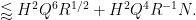
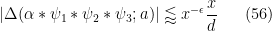
a sketch of his new Type III estimate with Fouvry, Michel, and Nelson. I will reproduce their argument in the notation of the blog post above. The objective is to obtain an estimate of the form
for as large as possible (in particular, as large as
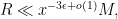
  ), but restricted to be square-free and
  -densely divisible. By the dense divisibility, it will suffice to show that
for that we can specify to accuracy
  , thus we may place
  in
in ![[x^{-\delta} R_0, R_0]](https://s0.wp.com/latex.php?latex=%5Bx%5E%7B-%5Cdelta%7D+R_0%2C+R_0%5D&bg=ffffff&fg=545454&s=0&c=20201002) for some
for some  to be chosen later, and
  .
.
FKMN do not exploit any averaging in or
or  ; one can probably exploit the former to improve upon their results but we will not do so here. Removing those averages, we are now looking at
This may be rewritten as
where does not depend on the residues
  , and the
  are bounded and only supported on those
  coprime to
  . Performing completion of sums in the
  variables, the left-hand side can be expressed as
plus terms which do not depend on (coming from the cases when at least one of the
  vanish), where
  and
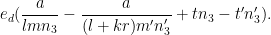
and  . The inner sum may be rescaled as
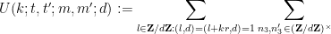
where is the hyper-Kloosterman sum
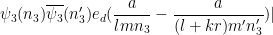
The now only appear through their product, and so we may gather terms and write the expression (*) as
where is the number of representations
  with
with  and
and  , and
, and  is another bounded sequence. The objective is now to show
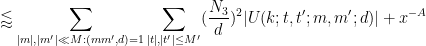
Note that . Deligne tells us that
  , which bounds the LHS by
  , but this only works in the Bombieri-Vinogradov regime
  . To do better we apply Cauchy-Schwarz to eliminate the
  term and gain another unweighted index
  to sum over. From the divisor bound one has
so it suffices to show that
We can rearrange the LHS as
The summand is periodic in h with period![[r_1,r_2] s](https://s0.wp.com/latex.php?latex=%5Br_1%2Cr_2%5D+s&bg=ffffff&fg=545454&s=0&c=20201002)
 , using the Chinese remainder theorem and Deligne’s estimates to estimate the completed sums, and eventually ends up with a bound on the inner sum of the form
One then performs completion of sums in
where and
and  . So now one has to sum
A computation shows that for each choice of and
and  , the number of pairs
  with
with  and
and  is
is  . So now one is summing
One can perform the summation without difficulty and end up with
and then performing the summation this becomes
The first term is bounded by the third and can be dropped. We also crudely bound the secondary term by
by  .
. , this is equivalent to requiring (ignoring epsilons)
To make this less than
The expression is a geometric average
  of the other two and so the
  term may be dropped. This already forces
  . As we may specify
  to accuracy
  , we win as soon as
which rearranges to
or equivalently
thus
In terms of , this gives a constraint
which can be rearranged as
We also have
If we play this against the Type I constraints
in the main post, one ends up with
leaving one with the final constraint
coming from merging the (1+3) and (2+4) estimates (this is not quite optimal, but will do for now).
This should be improvable once we flesh out the improved Type I estimates currently being discussed at https://terrytao.wordpress.com/2013/06/22/bounding-short-exponential-sums-on-smooth-moduli-via-weyl-differencing/ . But the fact that all the different combinations (1+3), …, (6) are beginning to surface means that we will have to start fighting on a lot of fronts to get more improvement from here on.
25 June, 2013 at 6:27 pm
Hannes
25 June, 2013 at 6:36 pm
David Roberts
And if confirmed, a prime gap bound of 7860.
25 June, 2013 at 9:26 pm
Terence Tao
confirmed by maple, going on the wiki :)
varpi := 1/116 - 0.62 / 10^5;
k0 := 1007;
deltap := 0.0085;
A := 396;
delta := (1 - 116 * varpi) / 30;
theta := deltap / (1/4 + varpi);
# Gergely's improved value for thetat
thetat := ((deltap - delta)/2 + varpi) / (1/4 + varpi);
deltat := delta / (1/4 + varpi);
j := BesselJZeros(k0-2,1);
eps := 1 - j^2 / (k0 * (k0-1) * (1+4*varpi));
kappa1 := int( (1-t)^((k0-1)/2)/t, t = theta..1, numeric);
kappa2 := (k0-1) * int( (1-t)^(k0-1)/t, t=theta..1, numeric);
# using Gergely and Eytan's improved kappa_3
alpha := j^2 / (4 * (k0-1));
e := exp( A + (k0-1) * int( exp(-(A+2*alpha)*t)/t, t=deltat..theta, numeric ) );
# using Gergely's exact expression for denominator
gd := (j^2/2) * BesselJ(k0-3,j)^2;
# using Eytan's exact expression for numerator
tn := sqrt(thetat)*j;
gn := (tn^2/2) * (BesselJ(k0-2,tn)^2 - BesselJ(k0-3,tn)*BesselJ(k0-1,tn));
kappa3 := (gn/gd) * e;
eps2 := 2*(kappa1+kappa2+kappa3);
# we win if eps2 < eps
25 June, 2013 at 10:57 pm
Hannes
Asking Maple for more digits (Digits := …) will cause this script to fail. However, I believe it will work after correcting the typo in the expression for delta. :-)
[Corrected, thanks – T.]
26 June, 2013 at 7:35 am
Terence Tao
Actually the treatment of the degenerate terms is a bit more difficult than I claimed, because the rescaling identity
is only true when are coprime to
  . One should be able to eliminate the non-coprime cases by introducing some “B” parameters as in the blog post treatment of the Type III case but it will get a bit messy. In principle it should work because whenever one or two of the
  share a common prime
  with
with  , one picks up two or one Ramanujan sums in the
  modulus which should safely counteract all the losses coming elsewhere from having to enforce such divisibility conditions. One also has to deal with the case when all of the
  have a common factor; this should be handled by factoring out these common factors from
  and inserting “B” terms to measure the losses and gains. In past experience there were always many powers of B to spare, so I don’t think this is a major issue, but it does need to be addressed at some point.
26 June, 2013 at 10:08 am
Terence Tao
OK, the treatment of the non-coprime case ends up being slightly tricky, one has to force coprimality before performing the factoring
  because one needs to optimise the factoring with respect to the common factor in order to get a convergent series.
Here are some details. The key estimate is
Proposition Let be of polynomial size. If
  are bounded and supported on
  -densely divisible squarefree
  , then
Proof By pigeonholing and dense divisbility we may factor with
with  ,
,  with
with
and
It then suffices to show that
for some bounded that is supported on coprime
  and
and  .
.
We pull the s summation out and then Cauchy-Schwarz in h to bound this by
The sum inside the parentheses can be estimated using the previous arguments as
so the LHS of (*) is
which we can rewrite as
and the claim then follows from the upper bounds on R,S.
Now back to the Type III estimates. We wish to show
where does not depend on the
  . After completion of sums and removing the degenerate frequencies, this becomes
where
would morally be the hyper-Kloosterman sum except that we do not yet have that
  are coprime to
  .
.
Suppose that . Writing
  ,
, ![b := [b_1,b_2,b_3]](https://s0.wp.com/latex.php?latex=b+%3A%3D+%5Bb_1%2Cb_2%2Cb_3%5D&bg=ffffff&fg=545454&s=0&c=20201002) and
and  , we can use the Chinese remainder theorem and Ramanujan sum bounds to factor
  as
as  times a factor independent of
  of magnitude
  (we skip this computation, it boils down to checking a bunch of cases when
  consists of a single prime
  ). For each fixed
  , we apply the Proposition with H replaced by
  and
and  replaced by
  , noting that the modulus
  is now only
  -densely divisible instead of
  -densely divisible, and one ends up with a total bound of
Fortunately, the net power of b here in the denominator is greater than 1, and the b summation converges (as can be seen by taking Euler products) to get a bound of
which is as required if
and we are back to the same numerology as before. So the coprimality thing is a moderate pain to deal with, but fortunately doesn’t seem to ultimately impact the final estimates.
26 June, 2013 at 7:51 am
Pace Nielsen
Plugging in the constraints (1+3), (1+4), (1+5), (2+3), (2+4), (2+5), and (6) into Mathematica’s “Reduce” function (which I love by the way) yields the final constraints (if I copied everything correctly):
or
or
26 June, 2013 at 10:15 am
Terence Tao
Thanks! There is also the trivial constraint which presumably kills off the third case here, so for the regime of
  we are currently shooting for, the
  condition is dominant.
2 July, 2013 at 9:47 am
Gergely Harcos
In the Wiki page (http://michaelnielsen.org/polymath1/index.php?title=Distribution_of_primes_in_smooth_moduli) the condition has been misprinted as
  .
.
[Fixed, thanks – T.]
26 June, 2013 at 10:26 am
Gergely Harcos
Can you share your code? Sounds like a nice function of Mathematica indeed.
26 June, 2013 at 10:56 am
Pace Nielsen
The code is actually quite simple which is why I like the function so much. If I had been thinking straight, I would have added the extra conditions , etc. The downside is that it is all automated, and so (in the final write-up) we may need to rederive the necessary inequalities. (But that shouldn't be too hard, given that we would know what to look for.)
All I typed was: Reduce[116p + (51/2)d<1 && 108p+25d<1 && … ]
This should be able to deal with any sort of polytope issues (at least for a small number of variables).
26 June, 2013 at 11:04 am
Hannes
An alternative is to just draw the lines… This is maple code:
with(plots):
eq := [116*varpi + 51/2*delta = 1,
108*varpi + 25*delta = 1,
412*varpi + 111*delta = 5,
280*varpi + 80*delta = 3,
100*varpi + 30*delta = 1,
160*varpi + 45*delta = 2,
96*varpi + 14*delta = 1]:
max_v := min(seq( eval(solve(e, varpi), delta=0), e in eq ));
max_d := min(seq( eval(solve(e, delta), varpi=0), e in eq ));
implicitplot(eq, varpi=0..max_v, delta=0..max_d, color=[blue,black,black,black,red,black,black]);
26 June, 2013 at 11:10 am
Gergely Harcos
Thank you guys, such tricks save time!
26 June, 2013 at 1:54 pm
Terence Tao
I found some Maple code (LinearMultivariateSystem) that does something similar, and allows me to plug in the Type I, Type II, and Type III constraints directly without having to manually play off the inequalities against each other. The (varpi,delta,sigma) polytope ends up being a bit messy but it does confirm that the main constraint is when
when  .
.
with(SolveTools[Inequality]);
base := [ sigma > 1/10, sigma < 1/2, varpi > 0, varpi < 1/4, delta > 0, delta < 1/4+varpi ];
typeI_1 := [ 11 * varpi + 3 * delta + 2 * sigma < 1/4 ];
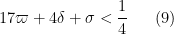
typeI_2 := [ 17 * varpi + 4 * delta + sigma < 1/4, 20 * varpi + 6 * delta + 3 * sigma < 1/2, 32 * varpi + 9 * delta + sigma < 1/2 ];
typeII_1 := [ 58 * varpi + 10 * delta < 1/2 ];
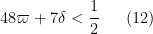
typeII_1a := [48 * varpi + 7 * delta < 1/2 ];
typeIII_1 := [ (13/2) * (1/2 + sigma) > 8 * (1/2 + 2*varpi) + delta ];
typeIII_2 := [ 1 + 5 * (1/2 + sigma) > 8 * (1/2 + 2*varpi) + delta ];
typeIII_3 := [ 3/2 * (1/2 + sigma) > (7/4) * (1/2 + 2*varpi) + (3/8) * delta ];
constraints := [ op(base), op(typeI_2), op(typeII_1a), op(typeIII_3) ];
LinearMultivariateSystem(constraints, [varpi,delta,sigma]);
25 June, 2013 at 7:00 pm
Terence Tao
This comment is an attempt to summarise the many different advances we have (whether worked out in full, or only partially sketched so far) on the problem of getting as large as possible. To simplify this overview I will not make a distinction between
 ![MPZ[\varpi,\delta]](https://s0.wp.com/latex.php?latex=MPZ%5B%5Cvarpi%2C%5Cdelta%5D&bg=ffffff&fg=545454&s=0&c=20201002) or
or ![MPZ'[\varpi,\delta]](https://s0.wp.com/latex.php?latex=MPZ%27%5B%5Cvarpi%2C%5Cdelta%5D&bg=ffffff&fg=545454&s=0&c=20201002) (so I will not distinguish between smoothness, dense divisibility, or “double dense divisibility”).
(so I will not distinguish between smoothness, dense divisibility, or “double dense divisibility”).
These estimates are obtained by a combination of three types of estimates: Type I estimates, Type II estimates, and Type III estimates. We have various levels of technological advance on each of these estimates, with a question mark indicating that this technology has not yet been fully fleshed out:
Type I-1: Zhang’s original argument bounding Type I estimates. Uses the bound on incomplete Kloosterman sums coming from completion of sums.
Type I-2: A refinement to Type I-1 coming from using q-van der Corput in the d_2 direction to improve the bounds on incomplete Kloosterman sums.
Type I-3?: A refinement to Type I-2 coming from refactoring the modulus d=d_1 d_2 to optimise the direction in which to apply q-van der Corput.
Type I-4?: A further refinement coming from iterating the q-van der Corput method.
Type I-5??: A yet further refinement taking advantage of additional averaging to reduce the contribution of diagonal terms.
Type II-1, Type II-2?, Type II-3?, Type II-4?, Type II-5??: Analogues of Type I-1 to Type I-5?? for the Type II sums.
Type III-1: Zhang’s original argument bounding Type III modulus, using Weyl differencing and not taking advantage of the alpha averaging.
Type III-2: Refinement of Type III-1 taking advantage of the alpha averaging to reduce the contribution of diagonal terms.
Type III-3: The new Fouvry-Kowalski-Michel argument avoiding Weyl differencing. Does not take advantage of the alpha averaging.
Type III-4?: Combining Fouvry-Kowalski-Michel with the alpha averaging.
Now a quick summary of progress so far:
* Zhang’s original argument uses Type I-1 + Type II-1 + Type III-1. This was optimised to give the constraint .
.
* By upgrading Type III-1 to Type III-2, we computed the numerology for Type I-1 + Type II-1 + Type III-2 and got .
.
* By upgrading Type I-1 to Type I-2, we computed the numerology for Type I-2 + Type II-1 + Type III-2 and got , as described in the post above. (I had earlier computed Type I-2 + Type II-1 + Type III-1 to get the inferior constraint
  .)
.)
* By upgrading Type I-2 to Type I-3?, and using Type I-3? + Type II-1 + Type III-2, we have tentatively computed either or
or  (this discrepancy is not yet resolved).
* A very sketchy projection of Type I-4? + Type II-1 + Type III-2 suggests that could get as large as 1/74 (or 1/88 if we only use Type III-1 instead of Type III-2), except that the Type II-1 estimates start failing at 1/96. However this can presumably be overcome by upgrading Type II-1 to something better, such as Type II-2? or Type II-3?; we have not yet bothered to do anything to the Type II sums but we should probably do so soon.
* In the comments above, I have worked out the numerology for Type I-2 + Type II-1 + Type III-3 and obtained .
.
Clearly there is a lot more progress to be made. Ideally we can work out the details of all the different estimates above and arrive at Type I-5 + Type II-5 + Type III-4 which should give significantly better values of than we currently have.
One can view each of these estimates as working on some polytope in parameter space, with
 ![MPZ[\varpi,\delta]](https://s0.wp.com/latex.php?latex=MPZ%5B%5Cvarpi%2C%5Cdelta%5D&bg=ffffff&fg=545454&s=0&c=20201002) (or some variant thereof) holding if one can find a
(or some variant thereof) holding if one can find a  such that
  simultaneously lies in a Type I-polytope, a Type II-polytope, and a Type III-polytope.
I think I will write up a wiki page to organise all this.
25 June, 2013 at 9:22 pm
Terence Tao
The wiki page is now up:
http://michaelnielsen.org/polymath1/index.php?title=Distribution_of_primes_in_smooth_moduli
In the next day or two I’ll start on systematically working out the various levels of Type I, Type II, and Type III estimates that we currently have, which should lead to a sequence of improvements to .
.
25 June, 2013 at 9:58 pm
aviwlevy
There seems to be a missing comment hyperlink under Type I, Level 4 on the new wiki page.
[Corrected, thanks – T.]
25 June, 2013 at 9:42 pm
Emmanuel Kowalski
I hope it is explicit enough in what I wrote on my blogs that we worked with Paul Nelson on this…
[Sorry about that! I’ve updated the attributions accordingly. -T.]
25 June, 2013 at 9:54 pm
Emmanuel Kowalski
Thanks; the summary page of the Wiki also has one mistake, and also the summary two comments above (Type III-3, Type III-4?)…
[Corrected, thanks – T.]
26 June, 2013 at 2:51 pm
Terence Tao
The purpose of this comment is to record the details of the “Level 3” Type I estimate, which optimises the direction in which the q-van der Corput A-process (aka Weyl differencing) is applied, in the context of densely divisible moduli. This was sketched already in https://terrytao.wordpress.com/2013/06/23/the-distribution-of-primes-in-densely-divisible-moduli but is done here a little more carefully (in particular, a secondary constraint on can now be shown to be dropped).
First, a convenient fact: if are both
  -densely divisible, then
 ![[a,b]](https://s0.wp.com/latex.php?latex=%5Ba%2Cb%5D&bg=ffffff&fg=545454&s=0&c=20201002) is also
is also  -densely divisible. This is because at least one of
  must be as large as
 ![[a,b]^{1/2}](https://s0.wp.com/latex.php?latex=%5Ba%2Cb%5D%5E%7B1%2F2%7D&bg=ffffff&fg=545454&s=0&c=20201002) ; if say
; if say  is this large then one can use the factors of
  , together with the factors of
  times
times ![[a,b]/a](https://s0.wp.com/latex.php?latex=%5Ba%2Cb%5D%2Fa&bg=ffffff&fg=545454&s=0&c=20201002) , to demonstrate the dense divisibility of
, to demonstrate the dense divisibility of ![[a,b]](https://s0.wp.com/latex.php?latex=%5Ba%2Cb%5D&bg=ffffff&fg=545454&s=0&c=20201002) .
.
In particular, in the context of Lemma 10 above, the quantity![q_1 r [q_2,q'_2]](https://s0.wp.com/latex.php?latex=q_1+r+%5Bq_2%2Cq%27_2%5D&bg=ffffff&fg=545454&s=0&c=20201002) is
is  -densely divisible, because
  are
are  -densely divisible by construction.
Next, a Kloosterman sum bound: if
with squarefree and coprime with
 -densely divisible, then for any other factorisation
  of
of  , we may use the k=1 van der Corput bound from this comment and bound
if , where
  ,
,  , and
, and  . If we choose a factorisation
  with
with  in this case, we end up with
In the opposite case when , we basically have from completion of sums that
(strictly speaking we need to improve to
to  to get something like this, but let’s ignore this detail) and by computing the degenerate completed Kloosterman sum we obtain a bound of
  here. So the net bound on
  is
is
Using this bound, we can improve the RHS in Lemma 10 of this post to
(one can get further improvements to the second term in the RHS by also studying the other components of and
and  , but I don’t think we need these improvements yet.) The non-diagonal contribution to (50) is then
which needs to be
leading to the conditions
and
As and
and  , this becomes
which since ,
,  , and
, and  for an infinitesimal
  , leads to the constraints
and
which may be rearranged as
and
The second constraint is clearly dominated by the first and so may be dropped. We conclude the “Level 3” bound that the Type I estimates hold for . Combining the Level 3 Type I estimates with the current best Type II estimate (which I’ve called Level 1a on the wiki) and the best Type III estimate (Level 3), Maple gives the slightly messy constraint
for
which is a little bit better than the previous bound of .
.
with(SolveTools[Inequality]);

base := [ sigma > 1/10, sigma < 1/2, varpi > 0, varpi < 1/4, delta > 0, delta < 1/4+varpi ];

typeI_1 := [ 11 * varpi + 3 * delta + 2 * sigma < 1/4 ];

typeI_2 := [ 17 * varpi + 4 * delta + sigma < 1/4, 20 * varpi + 6 * delta + 3 * sigma < 1/2, 32 * varpi + 9 * delta + sigma < 1/2 ];

typeI_3 := [ 54 * varpi + 15 * delta + 5 * sigma < 1 ];

typeII_1 := [ 58 * varpi + 10 * delta < 1/2 ];

typeII_1a := [48 * varpi + 7 * delta < 1/2 ];

typeIII_1 := [ (13/2) * (1/2 + sigma) > 8 * (1/2 + 2*varpi) + delta ];

typeIII_2 := [ 1 + 5 * (1/2 + sigma) > 8 * (1/2 + 2*varpi) + delta ];

typeIII_3 := [ 3/2 * (1/2 + sigma) > (7/4) * (1/2 + 2*varpi) + (3/8) * delta ];

constraints := [ op(base), op(typeI_3), op(typeII_1a), op(typeIII_3) ];

LinearMultivariateSystem(constraints, [varpi,delta,sigma]);
26 June, 2013 at 6:48 pm
Hannes
I think works.
26 June, 2013 at 7:04 pm
Terence Tao
Maple confirms, as usual… it gives H = 7470. Thanks!
k0 := 962;

varpi := 7/788 - 0.5932/10^5;

delta := (7 - 788*varpi) / 195;

deltap := 0.0069;

A := 388;

theta := deltap / (1/4 + varpi);

thetat := ((deltap - delta)/2 + varpi) / (1/4 + varpi);

deltat := delta / (1/4 + varpi);

j := BesselJZeros(k0-2,1);

eps := 1 - j^2 / (k0 * (k0-1) * (1+4*varpi));

kappa1 := int( (1-t)^((k0-1)/2)/t, t = theta..1, numeric);

kappa2 := (k0-1) * int( (1-t)^(k0-1)/t, t=theta..1, numeric);

alpha := j^2 / (4 * (k0-1));

e := exp( A + (k0-1) * int( exp(-(A+2*alpha)*t)/t, t=deltat..theta, numeric ) );

gd := (j^2/2) * BesselJ(k0-3,j)^2;

tn := sqrt(thetat)*j;

gn := (tn^2/2) * (BesselJ(k0-2,tn)^2 - BesselJ(k0-3,tn)*BesselJ(k0-1,tn));

kappa3 := (gn/gd) * e;

eps2 := 2*(kappa1+kappa2+kappa3);

# we win if eps2 < eps
27 June, 2013 at 9:48 am
Anonymous
There is a typo in the last line of the code, it should be constraints.
[Corrected, thanks – T.]
26 June, 2013 at 9:53 pm
Terence Tao
I’ve been looking at the Type II estimates. My plan was to mimic the “Level 2” and “Level 3” improvements for the Type I estimates to obtain analogous gains in Type II, but I found an interesting phenomenon, in that the critical numerology for the Type II estimates actually fall outside of the range in which the van der Corput type lemmas gain over the completion of sums bound, so the Level 2 and Level 3 estimates are actually worse than the Level 1 estimates. However, I was able to extract a different gain by observing that the parameter R, which currently in the Type II case is constrained to the interval
could instead be constrained to
(which, in retrospect, is closer to what Zhang did originally, though he used instead of
  ) and this gives slightly better numerology, improving the old constraint of
  to
to  . In a bit more detail, the two constraints coming out of the Type II analysis are
and
and if one inserts the bounds ,
,  , and
, and  one obtains the constraints
and
which lead to the stated constraint .
.
Setting , the critical numerology for Type 2 is then
  ,
,  ,
,  ,
,  ,
,  . In Lemma 11, the modulus
 ![d := r[q_1,q'_1,q_2,q'_2]](https://s0.wp.com/latex.php?latex=d+%3A%3D+r%5Bq_1%2Cq%27_1%2Cq_2%2Cq%27_2%5D&bg=ffffff&fg=545454&s=0&c=20201002) should be of size
should be of size  , while
  is of size
  , so
, so  , which is too large for a single van der Corput estimate to be useful (but potentially a combination of the A and B process might barely squeeze a slight gain in this regime).
27 June, 2013 at 4:45 am
Eytan Paldi
Perhaps the parameters ( ) defining the range of
  are still not the optimal ones? (if so, they may be optimized.)
27 June, 2013 at 8:59 am
Terence Tao
A good question!
The constraints on R arise in the following ways. Generally, one would like R to be as large as possible, as most of the bounds we need are of the form for various positive exponents
  , and various quantities
  that do not depend on R. (Ultimately, this is because R represents the portion of the modulus that we do not perform Cauchy-Schwarz on (when moving from (35) to (36) in the main post.) On the other hand, due to the
  -densely divisible hypothesis, we can only localise R to an interval of the form
 ![[x^{-\delta} R_0, R_0]](https://s0.wp.com/latex.php?latex=%5Bx%5E%7B-%5Cdelta%7D+R_0%2C+R_0%5D&bg=ffffff&fg=545454&s=0&c=20201002) , where we are free to choose
, where we are free to choose  . So we would generally like
  to be large as possible as well.
However, there is a “diagonal” contribution coming from the case when have a common factor which needs to also be addressed; this is only briefly mentioned in this post (near (38)), but is done in more detail in the treatment of (32) in https://terrytao.wordpress.com/2013/06/12/estimation-of-the-type-i-and-type-ii-sums/ . The treatment of this case is complicated, but produces three upper bounds required on R, namely
Note that these quantities also necessarily obey the conditions and
and  .
.
In the Type I case (when ) it is the first constraint that dominates, so that one sets
  for some small c. But in the Type II case (when
  ) it is the last case that dominates, so the largest
  can be here is
  .
.
However, it is possible that one could treat (32) a bit more efficiently. It seems unlikely that R could usefully ever be larger than N (otherwise it becomes pointless to try to Cauchy-Schwarz on the residue class ) but I don’t immediately have a good explanation as to why the condition (*) is so necessary. One might indeed be able to save a few more factors of
  this way.
27 June, 2013 at 9:40 am
Terence Tao
Actually, now that I look at it I think that (*) can indeed be removed, although it requires some technical modifications to the argument. Specifically, the controlled multiplicity hypothesis
(which should have been stated in this post, but was omitted accidentally) needs to be strengthened slightly to
but in the applications we need, this strengthening is available.
Henceforth all equation references are referring to https://terrytao.wordpress.com/2013/06/12/estimation-of-the-type-i-and-type-ii-sums/ .
We redo the estimation of the non-coprime contribution (32). Repeating the arguments in the previous post, we arrive at the task of bounding
by (plus a symmetric term that is treated similarly). As before, we crucially have that
  has no prime factors smaller than
  .
.
We now deviate from the previous post (which performed the m summation at this point) by introducing the new variable , which is comparable to x, and rearranging the above expression as
The sum is
  by crude estimates. By the divisor bound, the
  sum is then
  by crude bounds. By using the improved controlled multiplicity hypothesis (**), the
  sum is then
(noting that ), and then finally the
  sum is
and this is acceptable given the single condition
for some fixed . So we can set
  in both the Type I and Type II cases. Returning to the Type II analysis from my comment above, the constraints
and
should now be rearranged as
and
and using the bounds ,
,  and
and  , we are left with the constraints
and
which rearrange to
and
The second condition is redundant, leaving us with a "Level 1c" Type II constraint of , improving upon the previous constraint
  . Since even the most optimistic projections we have so far do not foresee
  going below 1/74, it now looks like the Type II estimates are good enough for the near-term that they will not cause any further difficulty.
Thanks for raising the question!
27 June, 2013 at 10:04 am
Eytan Paldi
I’m glad to see such fast improvement! (my last suggestion to optimize the parameters at the end of the project was sent before I read your response!)
Anyway, perhaps at the end of the project, it may be possible to optimize similar parameters when all the necessary limitations on them will become clear from the detailed proof.
27 June, 2013 at 9:45 am
Eytan Paldi
Perhaps such optimization (if possible) should be tried at the end of the project (when all the needed restrictions on the parameters will be known from the detailed proof.)
27 June, 2013 at 10:25 am
Pace Nielsen
I’ve been trying to figure out how the combinatorial lemma has influenced the creation of types 0,I,II,III; and conversely, how some natural cut-offs in estimating certain sums has influenced the creation of the combinatorial lemma. Further, I wanted to know if there was some sort of combinatorial improvement that could be made. In that spirit, let me describe how I now view things. This likely won’t be earthshattering for the experts, but may be helpful to those “occasional number-theorists” like myself.
For record keeping, let be coefficient sequences at scales
  , and let
  be smooth coefficient sequences at scales
  . We take positive real numbers
  such that
  and
and  . We also assume
  , and so
  . (Note: These real numbers are not fixed, but can change with
  . However, I’m postulating (from the answer to Avi Levy’s recent question), we can assume some sort of law of excluded middle, which I will use implicitly throughout this comment.) For simplicity, we assume
  and
and  . Furthermore, we may assume
  from how the coefficient sequences are created; the non-smooth sequences are (basically) convolutions of even smaller smooth sequences. (This assumption isn’t essential, but often helps simplify things.)
We want to estimate quantities (with possible future modifications to “doubly dense divisibility”) of the form
Intuitively speaking, we want more 's than
  's, since smoothness helps us. It is also my impression that we don't want too many terms in the Dirichlet convolution, or the sums is difficult to bound well. (But this is not always the case. For instance, the case
  is not always better than the Type I/II case where
  .) We often will combine some of the convolutions into a single term, but at the cost of sometimes losing smoothness. We say that the sum above is of signature
  .
.
Now come the combinatorics. I want to address two specific cases. First consider when . This is on the cups of what is not allowed using (the current) Type I-4 bounds. I believe that this will turn out to be a natural barrier, otherwise (as we'll see shortly) one could reprove Zhang's result without any Type III analysis.
Consider what happens when is large. Indeed, if
  then we are in the Type 0 case. What happens if
  is not quite so large? In the range
  we can reduce to the Type II regime, by combining all coefficient sequences except
  into a single term. Note that we have an added bonus; one of the two convolved functions is smooth! In the range
  we can similarly reduce to Type I, again with the bonus that the smaller of the two coefficient sequences is smooth.
Now, let's consider the other end of the spectrum, where is small. If
  then
then  for all
  . Thus, recombining the sequences we can reduce to signature
  where
where  . This is again Type I/II (but without the added bonus of at least one sequence being smooth). Further, when
  , this covers all possible cases.
Finally, we will look at the case when , which is outside the current combinatorial bounds. The cases when
  is large are dealt with in exactly the same way as above. Similarly, if
  , we can reduce to the Type I/II analysis as above. So, we reduce to the case when
  .
.
Zhang's combinatorial method here seems to consist of counting how many other 's can possibly belong to this same interval, while (without loss of generality) restricting
  , and further thinking of any
  as an
as an  (i.e. forgetting about the smoothness of such sequences).
(A) Suppose is the only
  in the given interval. Then
  , and taking just enough of the
  's and attaching them to
  , we reduce to Type I/II.
(B) Suppose are the only
  's in the given interval. Attaching all of the
  's to
's to  would give a sequence of size
  , and so there is some subcollection of the
  's which when attached to
  given a sequence of size between
  . Attaching the remainder of the
  's to
's to  reduces to Type I/II.
(C) If there are more than six 's in the interval, then we reach a contradiction since in that case
  .
.
(D) If there are exactly six 's in the interval, then we have
  . We reduce to type II by combining
  , and then combining the remaining sequences.
(E) If there are exactly five 's in the interval, then we have a new situation that wasn't covered by the combinatorial lemma. (This is one of the reasons for the cutoff at
  .) This can happen, for instance if
  . There are a few ways to deal with this new situation; depending on which of the signatures
  is most manageable.
(F) Suppose are the only
  's in the interval (and so
  ). If
). If  for some pair
  , then we reduce to Type I/II. If
  for every distinct pair, then
  . Thus, combining/convolving the sequences
  and all
  's, we have size
  . As in case (B), we reduce to Type I/II.
Thus, we reduce to when . If
. If  then we are in Type III (combining
  with all the
  's). So, we may also assume
  . Thus, we have
But and so
  . Thus
  . This situation is possible, for example when we have (approximately)
(G) Finally, consider the case when . As before, we may assume we *cannot* recombine and reduce to types I/II/III. If
  then we easily obtain
  and so
  . This easily reduces to Type I/II. So
  , and as we are not in Type III we have
  . As in (F), we can reduce to the case where
and so we also obtain, . This leaves
  . Thus, we can combine some of the
  's with
  , and reduce to Type I/II again. So there are no extra cases here.
Observations:———-
Can we improve on this? There are at least two ways to proceed; whether they improve things remains to be seen. Instead of counting the number of indices in the interval , we could continue with the (possibly more natural) process of considering signatures in order. So, for example, we might consider what happens for the signature
  (with the two smooth sequences having fairly "large" scales), and ply this against the Type III analysis. Indeed, this is somewhat suggested by the current form that the Type III computations take. Those estimate gives
  (where here we can take
  if we like, which we do). So, we want
  as large as possible (and hence we want
  ). Thus, we are naturally led to consider the case when there are two, nearly equal, large scales.
Another (possibly less helpful) option would be to consider signatures of the form . If we could do a Type III analysis without the smoothness hypothesis, this would remove the combinatorial constraint
  .
.
27 June, 2013 at 11:00 am
Terence Tao
Thanks for this analysis!
It’s a nice observation that the Type I/II case could stretch to cover all cases if could be raised to 1/4. This might lead to a simpler proof of Zhang’s theorem (in particular, not relying on Deligne’s version of the Weil conjectures, only Weil’s original results which nowadays can also be proven by elementary means) for sufficiently small
  by eliminating the Type III analysis. But for the task of getting
  as big as possible we presumably need an “all hands on deck” approach in which we throw all the estimates we have at the problem.
Actually, now that I think about it, might already be big enough for this purpose, as this is the meeting point between
  and
and  . So the Level 3 or Level 4 Type I estimates (combined with Type II) might already give a proof of Zhang’s theorem!
In the other direction, with regards to trying to push below 1/10, I think the two new critical cases to consider will be a “Type IV” sum in which n=4 and
  is close to
  and a “Type V” sum in which n=5 and
  is close to
  (I have not figured out exactly what “close to” means though). This basically corresponds to distribution results (for smooth or densely divisible moduli) for the higher order divisor functions
  and
and  . I am unsure if there are any fancy arguments in the literature (beyond the Zhang-based ones) that beat Bombieri-Vinogradov in this context; it seems that
  is pretty much state of the art. But this is certainly a good direction to focus attention on, though perhaps not by Polymath8; new ways to control
  and
and  would be very interesting beyond just the ability to squeeze a few more improvements to
  ,
,  , and
, and  . (I could imagine that Polymath8 eventually gets to the point where the
  constraint is the dominant obstruction, and then calls it a day, leaving it to others in the field to start attacking
  and
and  and get some improvements to
  etc. as a bonus.)
27 June, 2013 at 2:08 pm
Pace Nielsen
Yes, I believe that you are right that is already good enough (if you can deal with the “endpoint” case of
  ). It would be neat to see that lead to a simpler proof of Zhang’s theorem.
27 June, 2013 at 2:16 pm
Pace Nielsen
I see from your new Level 4 Type III analysis, that some of my observations may have been unwarranted. However, it still may be the case that those sums of signature naturally fit “inbetween” the Type I/II sums (whose signature is
  ) and the Type III sums (whose signature is
  ).
).
27 June, 2013 at 5:35 pm
David Roberts
If we can get to the point where is the main obstruction, where does that leave us with
  , taking all optimistic projections into account? And what about
  ?
?
27 June, 2013 at 7:20 pm
Terence Tao
Actually, with the Level 4 Type III estimates, we’ve just reached this point – so is basically stuck at 1/108 right now until we improve the Type I estimates again beyond Level 3. We do have an in principle improvement here (“Level 4”) by using an iterated van der Corput, but it is not yet implemented. In principle, this estimate give something like
  (ignoring deltas), so if we play that against
  that should give
  , though 3/200 ~ 1/67 is large enough that the Type II and Type III estimates will have to be improved again before we can actually reach this point.
28 June, 2013 at 5:40 am
xfxie
If , it is easily to obtain
  (e.g., for
  , based on a rough search using a simple nonlinear optimizer calling with the maple script), if the calculation is correct. This will totally fall into the region of Engelsma's exact bounds.
28 June, 2013 at 7:16 am
Anonymous
Unfortunately Xfxie the inequality in Tao’s comment is in “sigma” not “delta” the inequality above comes from the type 1 inequality and still needs to be confronted with type 3’s to eliminate sigma and get the final inequality. There is no delta in the inequality because he just wants a rough idea of the result (and because that factor wasn’t calculated yet).
Can you share the optimizer you are using I guess it could save some time here.
28 June, 2013 at 7:30 am
xfxie
@Anonymous: I have to reply here because cannot find the reply button under your thread.
The optimizer code is currently located on my home machine. I will try to post the code tonight or soon.
27 June, 2013 at 11:59 am
Terence Tao
In this comment I will upgrade another estimate, specifically to upgrade the “Level 3” Type III estimate of Fouvry, Kowalski, Michel, and Nelson to a “Level 4” estimate that exploits averaging in the alpha parameter to reduce the contribution of the diagonal terms (this idea was used in the “Level 2” estimates and was also suggested by FKMN). We will be largely repeating the arguments from the previous comment https://terrytao.wordpress.com/2013/06/23/the-distribution-of-primes-in-densely-divisible-moduli/#comment-236237 .
As in that comment, the objective is to show that
for that we can specify to accuracy
  , thus we may place
  in
in ![[x^{-\delta} R_0, R_0]](https://s0.wp.com/latex.php?latex=%5Bx%5E%7B-%5Cdelta%7D+R_0%2C+R_0%5D&bg=ffffff&fg=545454&s=0&c=20201002) for some
for some  to be chosen later, and
  .
.
FKMN discard the averaging in or
or  . For Level 4 estimates, we still discard the s averaging (there isn’t really any plausible way we know of to exploit it thus far) but keep the alpha average. We are now looking at
This may be rewritten as
where does not depend on the residues
  , and the
  are bounded and only supported on those
  coprime to
  . We can similarly restrict
  to those
  that are coprime to
  .
. variables, the left-hand side can be expressed as
Performing completion of sums in the
plus terms which do not depend on (coming from the cases when at least one of the
  vanish), where
  and
and  . Ignoring for this discussion the coprimality problem mentioned in a previous comment, the inner sum may be rescaled as
as before, so we may gather terms and write the expression (*) as
as before. The objective is now to show
By Cauchy-Schwarz as in the previous comment it suffices to show that
We can rearrange the LHS as
The summand is periodic in h with period![[r_1,r_2] s](https://s0.wp.com/latex.php?latex=%5Br_1%2Cr_2%5D+s&bg=ffffff&fg=545454&s=0&c=20201002)
 , using the Chinese remainder theorem and Deligne’s estimates to estimate the completed sums, and eventually ends up with a bound on the inner sum of the form
One then performs completion of sums in
where and
and  ; the insertion of the m factors is the key new improvement here. So now one has to sum
The diagonal case contributes a term of
by repeating the arguments from the previous comment. Now we turn to the off-diagonal contributions . Among other things this forces
  to divide
  , which already gives a noticeable gain (and forces
  to be only as large as
  ).
).
Fix . The same computation as the previous comment shows that for each choice of
  and
and  , the number of pairs
  with
with  and
and  is
is  . (There are
  choices for
  , and for fixed
  there are
  choices for
  .)
.)
So now one is summing
One can perform the summation without difficulty and end up with
and then performing the summation (which is now improved due to the constraint
  ) this becomes
Collecting terms, it is now
that we wish to be .
.
Ignoring epsilons, this gives rise to upper and lower bounds on R:
So we now have
Since has to be at least 1, we need
  , which also makes all the lower bounds on
  at most
  . We then win if
which rearranges to
These are stronger than the previous constraint which may now be discarded. Also the last constraint
  is weaker than
  and may also be dropped. As
  , the constraints may be rewritten as
thus
and
In terms of , this gives a constraint
which can be rearranged as
and
the first condition dominates, so it looks like the Level 4 Type III constraint is
which when combined with the latest Type I and Type II estimates (Level 3 and Level 1c respectively) seems to give the final constraint
which is basically formed by the collision of the constraint and the Level 3 Type I constraint of
  . Thus the Level 4 Type III estimates are so strong that they are no longer providing the dominant contribution, it is now the clash between Type I and the combinatorial constraint
  which is the bottleneck; Type III won’t become relevant again until
  hits 1/70. (This also means that the above analysis will be fairly robust to numerical errors.)
 with(SolveTools[Inequality]);

 base := [ sigma > 1/10, sigma  0, varpi  0, delta < 1/4+varpi ];

 typeI_1 := [ 11 * varpi + 3 * delta + 2 * sigma < 1/4 ];

 typeI_2 := [ 17 * varpi + 4 * delta + sigma < 1/4, 20 * varpi + 6 * delta + 3 * sigma < 1/2, 32 * varpi + 9 * delta + sigma < 1/2 ];

 typeI_3 := [ 54 * varpi + 15 * delta + 5 * sigma < 1 ];

 typeII_1 := [ 58 * varpi + 10 * delta < 1/2 ];

 typeII_1a := [48 * varpi + 7 * delta < 1/2 ];

 typeII_1b := [38 * varpi + 7 * delta < 1/2 ];

 typeII_1c := [34 * varpi + 7 * delta  8 * (1/2 + 2*varpi) + delta ];

 typeIII_2 := [ 1 + 5 * (1/2 + sigma) > 8 * (1/2 + 2*varpi) + delta ];

 typeIII_3 := [ 3/2 * (1/2 + sigma) > (7/4) * (1/2 + 2*varpi) + (3/8) * delta ];

 typeIII_4 := [ 3/2 * (1/2 + sigma) > (5/3) * (1/2 + 2*varpi) + (1/3) * delta ];

 constraints := [ op(base), op(typeI_3), op(typeII_1c), op(typeIII_4) ];

 LinearMultivariateSystem(constraints, [varpi,delta,sigma]);
27 June, 2013 at 12:45 pm
Hannes
Here I think one can choose .
.
27 June, 2013 at 2:38 pm
Terence Tao
Maple okays it :) Thanks to the shiny new narrow admissible tuples page (now accepting submissions!), this gives H = 6,966. (Four orders of magnitude improvement!)
k0 := 902;

varpi := 1/(6*18) - 0.735/10^5;

delta := (1/6 - 18*varpi)/5;

deltap := 0.0069;

A := 360;

theta := deltap / (1/4 + varpi);

thetat := ((deltap - delta)/2 + varpi) / (1/4 + varpi);

deltat := delta / (1/4 + varpi);

j := BesselJZeros(k0-2,1);

eps := 1 - j^2 / (k0 * (k0-1) * (1+4*varpi));

kappa1 := int( (1-t)^((k0-1)/2)/t, t = theta..1, numeric);

kappa2 := (k0-1) * int( (1-t)^(k0-1)/t, t=theta..1, numeric);

alpha := j^2 / (4 * (k0-1));

e := exp( A + (k0-1) * int( exp(-(A+2*alpha)*t)/t, t=deltat..theta, numeric ) );

gd := (j^2/2) * BesselJ(k0-3,j)^2;

tn := sqrt(thetat)*j;

gn := (tn^2/2) * (BesselJ(k0-2,tn)^2 - BesselJ(k0-3,tn)*BesselJ(k0-1,tn));

kappa3 := (gn/gd) * e;

eps2 := 2*(kappa1+kappa2+kappa3);

# we win if eps2 < eps
27 June, 2013 at 7:16 pm
Hannes
This script looks strange. Copy-error?
[Oops, the first three lines were missing; should be there now. -T.]
28 June, 2013 at 8:24 am
Pace Nielsen
Using this Level 4 Type III analysis, I have an idea [*very* sketchy at the moment] that has the potential to remove any reference to (thus removing Type I computations), unify Type 0 and Type III into a single result, and trivialize Type II computations.
Let us begin as above, but with the new objective to obtain the bound
Proceeding as in the comment, the main term of interest in the LHS is
Setting , and proceeding as before, the changes are twofold. First, replace
  by
by  . I believe that this causes no trouble, and can still be handled by the divisor bound. Second, we replace
  by
by  . Here is where my idea becomes especially sketchy. We need to find a bound on
of some manageable order. To continue, supposing we get something similar to
(which is what was obtained above in the case, possibly here with
  involving
  th powers), then the rest of the post seems to follow along similar lines. We still end with something *close* to the two conditions
and
These equations (when precisely stated) may now rely on , but for simplicity I’ll ignore that. Fix
  and restrict to the case
  . Considering all
  up to a large (but fixed) size, the only combinatorial case not covered is when all scales are smaller than
  . If
. If  is fine enough we can cover that final case with a Type II analysis (in a significantly shorter interval).
At any rate, it might be interesting to work out what happens when , as that will partially address the current
  obstruction.
28 June, 2013 at 8:47 am
Ph.M
I don’t know for the validity of the argument yet, but the Deligne type estimates for the K_n sums and product thereof possibly with an extra additive character (because polya-vinogradov) are valid exactly as for n=3 and are consequences of http://projecteuclid.org/DPubS?service=UI&version=1.0&verb=Display&handle=euclid.dmj/1077229697
28 June, 2013 at 8:51 am
Terence Tao
It is worth checking out the numerology for, say, n=4, ,
,  (even though this particular case can also be handled by Type II methods) and
  ,
,  to see if we can just beat Bombieri-Vinogradov for
  in the most favorable case by this method. I think the numerology may become a less favorable though (the normalisation of
  for instance, should have a factor of
  in front rather than
  to reflect the expected square root cancellation). There is also the additional issue that a certain amount of algebraic geometry (ell-adic sheaf cohomology, this sort of thing) is needed to actually justify the expected square root cancellation for sums such as
  but we can cross that bridge when we come to it.
28 June, 2013 at 9:10 am
Ph.M
As said above algebraic geometry is not at all a problem here; my greatest worry as you said is that will get huge if
  is large so that an important term in Polya-Vinogradov will be the zero frequency: for these one need a weight dropping phenomenon (more than square-root cancellation) for the complete sums,
  say,
say,
and
where : these sums can probably be evaluated in an elementary way and then their size may determine whether this has a chance for
  .
.
28 June, 2013 at 12:23 pm
Pace Nielsen
Thanks for the pointers. It looks like this idea won’t work out, but it gives me good motivation to understand the arguments better.
If it does turn out that gives a natural barrier, there is yet another way to beat the combinatorial restriction. If we are not in type 0,I,II, then we can still reduce to the case where there exist at least three real numbers in the range
  . In general, we no longer have that
  , but we can use the poorer lower bound
  . Unfortunately, with the current Level 4 Type III bounds, this gives
so it doesn’t help us (yet).
28 June, 2013 at 2:55 pm
Terence Tao
After a nice discussion over lunch with Philippe Michel (who happens to be in LA currently), I now have a clearer idea of why the Type III argument of FKMN beats Bombieri-Vinogradov for n=3 but just barely fails to do so for n=4.
Let’s start with n=3, taking and
and  for simplicity (so we are just at the border of Bombieri-Vinogradov. Philippe pointed out that it is convenient to write things in terms of powers of Q, thus
  here. We want to understand the expression
on the average for typical (smooth) (I will suppress the dependence of
  on
on  here for simplicity). The trivial bound here is
  , so we want to control this sum with accuracy
  or better. Using completion of sums, we can rewrite the above expression (morally) as
which (if we discard the cases where vanishes or otherwise has a common factor with
  ) is basically
(the out the front is absorbed into the normalisation of
  . Deligne (for the surface
  ) tells us that
  , giving us back
  . So a direct application of Deligne only recovers the trivial bound; but once we do even a little bit of Cauchy-Schwarz and take advantage of the averaging in q we can do better (again using Deligne, but now for a hyper-Kloosterman correlation rather than for a single hyper-Kloosterman sum). Eventually it turns out that we can get
  as low as
  (down from the current level of
  ), which corresponds to a 4/7 level of distribution.
Now we take n=4, in the model case when and
and  . We are now staring at
(before averaging in q). The trivial bound is as before. After completion of sums we get
(note here that completion of sums did not shorten the length of incomplete summation, in contrast to the n=3 case when it reduced a sum of length
  to the dual length of
  . With the normalisation of
  (which now has a
  in front instead of
  ), this morally becomes
Deligne still tells us that , but this now gives a net bound of
  , so we fall short by
  of even recovering Bombieri-Vinogradov here. We can _barely_ recover this by averaging in q as per FKMN. Namely, we are now trying to prove something like
for some bounded and some divisor-like function
  . Performing Cauchy-Schwarz in h, this becomes
The diagonal term is barely acceptable, and the off-diagonal terms are also barely accceptable using hyper-Kloosterman correlation (if we replace
  with
with  ). So we can barely recover Bombieri-Vinogradov with basically no room to maneuver. So it looks like we would have to come up with a new trick in order to use this sort of argument to get something non-trivial in the n=4 case.
28 June, 2013 at 4:38 pm
Gergely Harcos
Is it or
or  in the completed sum?
[It’s ; I’ve corrected the text. -T]
28 June, 2013 at 4:54 pm
Ph.M
What about doing this analysis with Cauchy in (h,r) (instead of h alone) with q=rs with r very small but >1 and s close to Q ?
28 June, 2013 at 8:12 pm
Terence Tao
Dear Philippe,
If we try to Cauchy-Schwarz in more variables, the off-diagonal terms become better, but the diagonal terms
  become worse; since both the diagonal and off-diagonal terms barely make it to Bombieri-Vinogradov, I don’t see a way to rebalance the Cauchy-Schwarz to do better. A little more precisely, we now write the Bombieri-Vinogradov type estimate to be proven as
with . If we Cauchy-Schwarz in h,r as you suggest we end up with
The diagonal contribution now has size
  which is now a little bit too big to even get back Bombieri-Vinogradov.
Having said this, though, I think this rebalancing trick may work for the Type I and Type II sums to get a further gain from what we already have (or plan to have). In both the Type I and Type II sums, one is eventually looking at a sum of the form
where is a certain explicit phase and the coefficients
  are essentially bounded (and never mind what k and r are, it’s not important for this discussion); see equation (39) of https://terrytao.wordpress.com/2013/06/12/estimation-of-the-type-i-and-type-ii-sums/ . In the Type I sum, Zhang performs Cauchy-Schwarz in the
  variables and finds that the diagonal terms
  are OK (as long as
  or equivalently
  for some small fixed
  ) and then works hard to control the off-diagonal terms
  . In the Type II sum, the diagonal terms
  coming from Cauchy-Schwarz in
  are no longer OK and so Zhang uses Cauchy-Schwarz in just
  in order to make the diagonal terms
  better, at the cost of making the off-diagonal terms
  worse (but because in Type II,
  and
and  are much closer to
  than in Type I, one still can get reasonable estimates here.
But in light of your suggestion, I see that there are other Cauchy-Schwarz’s available: in particular,in Type I we can factor and Cauchy-Schwarz in
  rather than just
  in order to make the diagonal terms do a bit more of the work and the off-diagonal terms do a bit less of the work. Similar optimisations are available in the Type II case (indeed one could imagine that one could now treat Type I and Type II in a unified fashion with a continuum of Cauchy-Schwarz options).
I’ll add this idea to the queue of possible Type I/Type II improvements (I’ll dub it “Level 6”). There are still two earlier potential Type I/Type II improvements (which I’ve called “Level 4” and “Level 5”) that should be worked out too; I think I can get a preliminary version of Level 4 worked out soon and will post it here. (It’s sort of a strange situation to have more ideas for progress than time available to work the ideas out properly; it’s almost always the other way around :-).)
27 June, 2013 at 6:18 pm
Mark Bennet
As someone who is following the discussion here with some interest, can I suggest that the constraints in current form would be easier to follow and compare when reading posts and tables (eg on the wiki page) if they were normalised to (ie clear fractions)
[Fair enough – I’ve edited the wiki accordingly. -T]
28 June, 2013 at 9:24 pm
Terence Tao
In this comment I am recording a preliminary “Level 4” estimate for Type I. However I am punting on the issue of exactly how to define “double dense divisibility” (which should roughly capture the notion that a modulus can be factored as
  with
with  placed more or less wherever one wants) and revert to the older notion of
  -smoothness. This will worsen the numerology when converting from
  to
to  (basically, this forces one to take
  , so that
  vanishes and
  is irrelevant) but I think the gain from improving
  will still be greater than the loss from having to revert to a more primitive sieve. (This is presumably a temporary issue, that can be resolved once we work out what double dense divisibility should be.) Unfortunately I have bad news – due to arithmetic errors in my previous projection at https://terrytao.wordpress.com/2013/06/22/bounding-short-exponential-sums-on-smooth-moduli-via-weyl-differencing/#comment-236039 , this argument ends up being a lot worse than anticipated, and in fact is inferior to the Level 3 estimate.
Anyway, to the details. As with this previous comment https://terrytao.wordpress.com/2013/06/23/the-distribution-of-primes-in-densely-divisible-moduli/#comment-236387 , the starting point is a bound for the incomplete Kloosterman sum
with squarefree and coprime with
 -smoooth, then for any other factorisation
  of
of  , we may use the k=2 van der Corput bound from this comment and bound
if , where
  ,
,  ,
,  , and
, and  . As
. As  is
is  -smooth, we may choose a factorisation
  with
with
and
(note that , so
, so  ) so that
and thus
Using completion of sums to handle the opposite case as in the previous comment, we conclude that
Using this bound, we can improve the RHS in Lemma 10 of this post to
The non-diagonal contribution to (50) is then
which needs to be
leading to the conditions
and
As and
and  , this becomes
which since ,
,  , and
, and  for an infinitesimal
  , leads to the constraints
and
which may be rearranged as
and
The second constraint is clearly dominated by the first and so may be dropped. We conclude the “Level 4” bound that the Type I estimates hold for . This is significantly worse than the previous claim of
  coming from https://terrytao.wordpress.com/2013/06/22/bounding-short-exponential-sums-on-smooth-moduli-via-weyl-differencing/#comment-236039 ; there were two arithmetic errors in the previous analysis, namely that a factor of
  actually should have been
  , and also an expression
  should have been
  . Playing this estimate off against the combinatorial constraint
  gives
gives  , which is a little worse than what we currently have. The moral here seems to be that the small gain coming from the second van der Corput is not quite strong enough to compensate for the large number of additional factors of
  one loses when trying to use that estimate.
On the plus side, it means that we don't have to think about double dense divisibility immediately…
29 June, 2013 at 4:42 am
Eytan Paldi
In the page “distribution of primes in smooth moduli” the coefficient of
 should be
  .
.
[Corrected, thanks – T.]
29 June, 2013 at 5:25 am
Gergely Harcos
A comment and a typo:
1. Besides (38), we also need the hypothesis , which is (33) from the earlier thread (https://terrytao.wordpress.com/2013/06/12/estimation-of-the-type-i-and-type-ii-sums/). This is automatic from (31) when
  are not too close to
  , e.g. under (48), but it requires
  in general. If (48) fails, then we choose
  , which is admissible.
2. “(45), (46), (49)” should be “(45), (46), (47)”: 3 occurrences.
[Corrected, thanks – T.]
29 June, 2013 at 10:31 am
Gergely Harcos
I thought we had to be a bit more careful about . Clearly,
  holds for
  small enough, but “small enough” really means “depending on
  “. On the other hand, in deriving Theorem 6 from Theorems 8 and 9, we make a choice of
  depending on
  . So without further comment,
  and
and  depend mutually on each other and the two dependencies might be contradictory. So I thought we had to make sure that for the choice of
  we make,
  is sufficiently small relative to it so that
  holds. This is why I said that assuming (48) any
  is good, while not assuming (48) any
  is good. Sorry if I am missing something. I wish you a good trip!
29 June, 2013 at 11:02 am
Terence Tao
Ah, I see what you are saying now. What’s happening is that I’m using c for two independent small quantities; I’ll change the second c to c’ to avoid circular dependenices.
29 June, 2013 at 11:45 am
Gergely Harcos
Thank you, it is clear now!
29 June, 2013 at 7:53 am
Terence Tao
I am beginning to suspect that the Type I/II analysis could be simplified by removing the somewhat intricate arguments Zhang uses to enforce that are coprime. (This would also remove the “controlled multiplicity” hypothesis from the congruence classes, and also remove most of the upper bound constraints on
  , potentially leading to some improvement in the numerology.) I have to check the details, but I think one of the main reasons Zhang needed coprimality (other than to make certain formulae look nicer) is that his exponential sum estimate on incomplete Kloosterman sums (Lemma 11 from Zhang’s paper) was a bit inefficient in the non-coprime case (his factors of
  in that Lemma should really be
  where
where  ). Otherwise, having common factors between the q’s actually _helps_ the analysis by making the overall modulus
 ![r[q_1,q_2,q'_2]](https://s0.wp.com/latex.php?latex=r%5Bq_1%2Cq_2%2Cq%27_2%5D&bg=ffffff&fg=545454&s=0&c=20201002) smaller. Again, I have to check the details…
smaller. Again, I have to check the details…
p.s. I’m leaving for Budapest today, probably will be out of action here for a day or so.
29 June, 2013 at 10:55 am
Terence Tao
OK, I now see where coprimality is really used. If one skips the reduction to the coprime case in the Type I/II analysis, one eventually has a little difficulty with the “main term”
  in the analysis (the display after (36) in https://terrytao.wordpress.com/2013/06/12/estimation-of-the-type-i-and-type-ii-sums/ ), which becomes
The problem comes from the new factor , which in the non-coprime case depends on the choice of
  and so cannot actually be dumped into the main term
  in the non-coprime case. However in that case one can estimate this expression crudely, using
  , as
, as
and on averaging in k we and using the lower bound we can show that this expression is (barely) acceptable as an error term rather than a main term. So we can’t get rid of the reduction that makes
  free of tiny primes. On the other hand, by reworking the argument in the above way we can avoid the need to assume controlled multiplicity altogether in Zhang’s theorem, thus strengthening it slightly.
I also now see that the condition is necessary for the dispersion method to work, otherwise the condition
  basically determines
  from
from  and there is nothing to disperse!
30 June, 2013 at 12:39 pm
Bounded gaps between primes (Polymath8) – a progress report | What's new
[…] sketch of Zhang’s argument for establishing Type I estimates (details may be found at these two posts). It is based on previous arguments of Bombieri, Friedlander, and Iwaniec, relying on various […]
30 June, 2013 at 12:40 pm
Terence Tao
Rolling over to a new thread at https://terrytao.wordpress.com/2013/06/30/bounded-gaps-between-primes-polymath8-a-progress-report/ (we traditionally do this every 100 comments or so, but the comments in this thread are particularly lengthy and technical and so I thought it would be good to recap with a fresh thread).
30 June, 2013 at 3:56 pm
Gergely Harcos
I think that Theorem 8 can be improved in that (47) can be omitted. We observe first that (52) can be supplemented by
as follows from the explicit formula
Using also , the last term in (51) can be improved to
The improvement is really by a factor of , since
  . By going back to earlier parts of the argument, we see that we need to average this over
  , and then sum over
  with
with  . This way we gain a factor of
  over the original contribution of the last term in (51). Therefore, instead of
we only need to ensure
that is,
In short, the last display of Section 3 can be replaced by
which rearranges to
So this would replace (47), but it follows from (45), hence can be omitted.
I hope I did not make a mistake. I also report two typos:
1. In the line before (52),![d_2:=[q_1,q_2]](https://s0.wp.com/latex.php?latex=d_2%3A%3D%5Bq_1%2Cq_2%5D&bg=ffffff&fg=545454&s=0&c=20201002) should be
should be ![d_2:=[q_2,q_2']](https://s0.wp.com/latex.php?latex=d_2%3A%3D%5Bq_2%2Cq_2%27%5D&bg=ffffff&fg=545454&s=0&c=20201002) .
.
2. In the fifth display of Section 6 of https://terrytao.wordpress.com/2013/06/12/estimation-of-the-type-i-and-type-ii-sums/, should be
  .
.
[Corrected, thanks. It looks like this improvement does not make the dominant inequalities any better, at least currently, but it may become useful at some later stage. -T]
4 July, 2013 at 11:55 pm
Gergely Harcos
Just a minor comment. In the last line in the proof of Lemma 11, “since divides
  but not
  ” should be “since
  divides
  but is coprime to
  “.
“.
[Corrected, thanks – T.]
7 July, 2013 at 11:17 pm
The distribution of primes in doubly densely divisible moduli | What's new
[…] improves upon the previous constraint of (see this previous post), although that latter statement was stronger in that it only required single dense divisibility […]
8 July, 2013 at 3:03 pm
Gergely Harcos
Just a typo: in (36), should be
  .
.
[Corrected, thanks – T.]
10 July, 2013 at 7:13 pm
Gergely Harcos
A question and some typos:
1. In the third display below Proposition 12, we have the constraint . Why is it not
  as dictated by
  from the previous display?
2. In the first display below Proposition 12, should be
  .
.
3. In the second and third display below Proposition 12, should be
  .
.
4. In the display following (63), should be
  .
.
[Corrected, thanks. The additional constraint does indeed need to be placed on
  but this is harmless as one simply applies Proposition 12 with a suitably truncated version of
  . -T]
. -T]
11 July, 2013 at 5:25 am
Gergely Harcos
Another question and two typos:
1. In the discussion below Proposition 12, you say that (62) with the appropriate parameters follows from (17). My calculation tells me that instead of (17) we need the slightly stronger bound . More precisely, we want
Am I missing something?
2. “values coprime to ” should be “values coprime to
  “.
“.
3. In (63) and in the display before (64), should be
  .
.
[Corrected, thanks. Increasing to
to  causes some changes in the final calculations, but fortunately only for non-dominant inequalities, and the final constraint on
  remains unchanged. -T.]
11 July, 2013 at 8:26 pm
Gergely Harcos
A few suggestions and typos:
1. In (66) and subsequent displays, I would put into parentheses.
2. In the proof of Proposition 12 you remark that (59) implies . I think (59) only implies
  , so the subsequent bound for
  needs an extra factor of
  .
.
3. In the three display following (71), the condition is missing, and
  should be
  .
.
4. In the second display below (71), a factor is missing on the right hand side.
5. In the third display below (72), the term is missing. Also, for the sake of the reader, it would be better to use the variables
  instead of
  in this definition.
6. In the fourth display below (72), the condition is missing.
7. In (74) and in the third display below (77), should be
  .
.
8. For the sake of the reader I would add more detail regarding the choice of below (77). There is a constant
  such that
  exceeds
  . If
. If  , then there is a divisor
  such that
  , and any such divisor is admissible by
  . Otherwise
  , hence
  is admissible by
  .
.
[Corrected, thanks – T.]
12 July, 2013 at 9:09 am
Gergely Harcos
Dear Terry, sorry for the trouble or if I am wrong, but:
1. We also need to change to
to ![|n_2 h' - n'_2 h|/d\in\mathbb{Z}\cap[0,O(x^\epsilon)]](https://s0.wp.com/latex.php?latex=%7Cn_2+h%27+-+n%27_2+h%7C%2Fd%5Cin%5Cmathbb%7BZ%7D%5Ccap%5B0%2CO%28x%5E%5Cepsilon%29%5D&bg=ffffff&fg=545454&s=0&c=20201002) in the second display before (71) and the line that precedes it.
in the second display before (71) and the line that precedes it.
2. In the fourth display below (72), the condition should be
  .
.
3. In the third display below (77), should be
  .
.
[Corrected, thanks – T.]
12 July, 2013 at 9:53 am
Gergely Harcos
Somehow these last corrections have not appeared, perhaps due to an upload problem?
[Oops, sorry about that – it should be OK now – T]