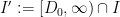
The distribution of primes in doubly densely divisible moduli

7 July, 2013 in math.NT, polymath | Tags: exponential sums, polymath8 | by Terence Tao

As in previous posts, we use the following asymptotic notation: ${x}$ is a parameter going off to infinity, and all quantities may depend on ${x}$ unless explicitly declared to be “fixed”. The asymptotic notation ${O(), o(), \ll}$ is then defined relative to this parameter. A quantity ${q}$ is said to be of polynomial size if one has ${q = O(x^{O(1)})}$ , and bounded if ${q=O(1)}$ . We also write ${X \lessapprox Y}$ for ${X \ll x^{o(1)} Y}$ , and ${X \sim Y}$ for ${X \ll Y \ll X}$ .

The purpose of this post is to collect together all the various refinements to the second half of Zhang’s paper that have been obtained as part of the polymath8 project and present them as a coherent argument. In order to state the main result, we need to recall some definitions. If ${I}$ is a bounded subset of ${{\bf R}}$ , let ${{\mathcal S}_I}$ denote the square-free numbers whose prime factors lie in ${I}$ , and let ${P_I := \prod_{p \in I} p}$ denote the product of the primes ${p}$ in ${I}$ . Note by the Chinese remainder theorem that the set ${({\bf Z}/P_I{\bf Z})^\times}$ of primitive congruence classes ${a\ (P_I)}$ modulo ${P_I}$ can be identified with the tuples ${(a_q\ (q))_{q \in {\mathcal S}_I}}$ of primitive congruence classes ${a_q\ (q)}$ of congruence classes modulo ${q}$ for each ${q \in {\mathcal S}_I}$ which obey the Chinese remainder theorem

$\displaystyle (a_{qr}\ (qr)) = (a_q\ (q)) \cap (a_r\ (r))$

for all coprime ${q,r \in {\mathcal S}_I}$ , since one can identify ${a\ (P_I)}$ with the tuple ${(a\ (q))_{q \in {\mathcal S}_I}}$ for each ${a \in ({\bf Z}/P_I{\bf Z})^\times}$ .

If ${y > 1}$ and ${n}$ is a natural number, we say that ${n}$ is ${y}$ -densely divisible if, for every ${1 \leq R \leq n}$ , one can find a factor of ${n}$ in the interval ${[y^{-1} R, R]}$ . We say that ${n}$ is doubly ${y}$ -densely divisible if, for every ${1 \leq R \leq n}$ , one can find a factor ${m}$ of ${n}$ in the interval ${[y^{-1} R, R]}$ such that ${m}$ is itself ${y}$ -densely divisible. We let ${{\mathcal D}_y^2}$ denote the set of doubly ${y}$ -densely divisible natural numbers, and ${{\mathcal D}_y}$ the set of ${y}$ -densely divisible numbers.

Given any finitely supported sequence ${\alpha: {\bf N} \rightarrow {\bf C}}$ and any primitive residue class ${a\ (q)}$ , we define the discrepancy

$\displaystyle \Delta(\alpha; a \ (q)) := \sum_{n: n = a\ (q)} \alpha(n) - \frac{1}{\phi(q)} \sum_{n: (n,q)=1} \alpha(n).$

For any fixed ${\varpi, \delta > 0}$ , we let ${MPZ''[\varpi,\delta]}$ denote the assertion that

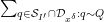
$\displaystyle \sum_{q \in {\mathcal S}_I \cap {\mathcal D}_{x^\delta}^2: q \leq x^{1/2+2\varpi}} |\Delta(\Lambda 1_{[x,2x]}; a\ (q))| \ll x \log^{-A} x \ \ \ \ \ (1)$

for any fixed ${A > 0}$ , any bounded ${I}$ , and any primitive ${a\ (P_I)}$ , where ${\Lambda}$ is the von Mangoldt function. Importantly, we do not require ${I}$ or ${a}$ to be fixed, in particular ${I}$ could grow polynomially in ${x}$ , and ${a}$ could grow exponentially in ${x}$ , but the implied constant in (1) would still need to be fixed (so it has to be uniform in ${I}$ and ${a}$ ). (In previous formulations of these estimates, the system of congruence ${a\ (q)}$ was also required to obey a controlled multiplicity hypothesis, but we no longer need this hypothesis in our arguments.) In this post we will record the proof of the following result, which is currently the best distribution result produced by the ongoing polymath8 project to optimise Zhang’s theorem on bounded gaps between primes:

Theorem 1 We have ${MPZ''[\varpi,\delta]}$ whenever ${\frac{280}{3} \varpi + \frac{80}{3} \delta < 1}$ .

This improves upon the previous constraint of ${148 \varpi + 33 \delta < 1}$ (see this previous post), although that latter statement was stronger in that it only required single dense divisibility rather than double dense divisibility. However, thanks to the efficiency of the sieving step of our argument, the upgrade of the single dense divisibility hypothesis to double dense divisibility costs almost nothing with respect to the ${k_0}$ parameter (which, using this constraint, gives a value of ${k_0=720}$ as verified in these comments, which then implies a value of ${H = 5,414}$ ).

This estimate is deduced from three sub-estimates, which require a bit more notation to state. We need a fixed quantity ${A_0>0}$ .

Definition 2 A coefficient sequence is a finitely supported sequence ${\alpha: {\bf N} \rightarrow {\bf R}}$ that obeys the bounds

$\displaystyle |\alpha(n)| \ll \tau^{O(1)}(n) \log^{O(1)}(x) \ \ \ \ \ (2)$

for all ${n}$ , where ${\tau}$ is the divisor function.

(i) A coefficient sequence ${\alpha}$ is said to be at scale ${N}$ for some ${N \geq 1}$ if it is supported on an interval of the form ${[(1-O(\log^{-A_0} x)) N, (1+O(\log^{-A_0} x)) N]}$ .

(ii) A coefficient sequence ${\alpha}$ at scale ${N}$ is said to obey the Siegel-Walfisz theorem if one has
$\displaystyle | \Delta(\alpha 1_{(\cdot,q)=1}; a\ (r)) | \ll \tau(qr)^{O(1)} N \log^{-A} x \ \ \ \ \ (3)$

for any ${q,r \geq 1}$ , any fixed ${A}$ , and any primitive residue class ${a\ (r)}$ .

(iii) A coefficient sequence ${\alpha}$ at scale ${N}$ (relative to this choice of ${A_0}$ ) is said to be smooth if it takes the form ${\alpha(n) = \psi(n/N)}$ for some smooth function ${\psi: {\bf R} \rightarrow {\bf C}}$ supported on ${[1-O(\log^{-A_0} x), 1+O(\log^{-A_0} x)]}$ obeying the derivative bounds
$\displaystyle \psi^{(j)}(t) = O( \log^{j A_0} x ) \ \ \ \ \ (4)$

for all fixed ${j \geq 0}$ (note that the implied constant in the ${O()}$ notation may depend on ${j}$ ).

Definition 3 (Type I, Type II, Type III estimates) Let ${0 < \varpi < 1/4}$ , ${0 < \delta < 1/4+\varpi}$ , and ${0 < \sigma < 1/2}$ be fixed quantities. We let ${I}$ be an arbitrary bounded subset of ${{\bf R}}$ , and ${a\ (P_I)}$ a primitive congruence class.

(i) We say that ${Type''_I[\varpi,\delta,\sigma]}$ holds if, whenever ${M, N \gg 1}$ are quantities with
$\displaystyle M N \sim x \ \ \ \ \ (5)$

and

$\displaystyle x^{1/2-\sigma} \lessapprox N \lessapprox x^{1/2-2\varpi-c} \ \ \ \ \ (6)$

for some fixed ${c>0}$ , and ${\alpha,\beta}$ are coefficient sequences at scales ${M,N}$ respectively, with ${\beta}$ obeying a Siegel-Walfisz theorem, we have

$\displaystyle \sum_{q \in {\mathcal S}_I \cap {\mathcal D}_{x^\delta}^2: q \leq x^{1/2+2\varpi}} |\Delta(\alpha * \beta; a\ (q))| \ll x \log^{-A} x. \ \ \ \ \ (7)$

(ii) We say that ${Type''_{II}[\varpi,\delta]}$ holds if the conclusion (7) of ${Type''_I[\varpi,\delta,\sigma]}$ holds under the same hypotheses as before, except that (6) is replaced with
$\displaystyle x^{1/2-2\varpi-c} \lessapprox N \lessapprox x^{1/2} \ \ \ \ \ (8)$

for some sufficiently small fixed ${c>0}$ .

(iii) We say that ${Type''_{III}[\varpi,\delta,\sigma]}$ holds if, whenever ${M, N_1,N_2,N_3 \gg 1}$ are quantities with
$\displaystyle M N_1 N_2 N_3 \sim x$

and

$\displaystyle N_1 N_2, N_1 N_3, N_2 N_3 \gtrapprox x^{1/2+\sigma} \ \ \ \ \ (9)$

and

$\displaystyle x^{2\sigma} \lessapprox N_1,N_2,N_3 \lessapprox x^{1/2-\sigma} \ \ \ \ \ (10)$

and ${\alpha,\psi_1,\psi_2,\psi_3}$ are coefficient sequences at scales ${M,N_1,N_2,N_3}$ respectively, with ${\psi_1,\psi_2,\psi_3}$ smooth, we have

$\displaystyle \sum_{q \in {\mathcal S}_I \cap {\mathcal D}_{x^\delta}^2: q \leq x^{1/2+2\varpi}} \ \ \ \ \ (11)$

$\displaystyle |\Delta(\alpha * \psi_1 * \psi_2 * \psi_3; a\ (q))| \ll x \log^{-A} x.$

Theorem 1 is then a consequence of the following four statements.

Theorem 4 (Type I estimate) ${Type''_I[\varpi,\delta,\sigma]}$ holds whenever ${\varpi,\delta,\sigma > 0}$ are fixed quantities such that

$\displaystyle 56 \varpi + 16 \delta + 4\sigma < 1.$

Theorem 5 (Type II estimate) ${Type''_{II}[\varpi,\delta]}$ holds whenever ${\varpi,\delta > 0}$ are fixed quantities such that

$\displaystyle 68 \varpi + 14 \delta < 1.$

Theorem 6 (Type III estimate) ${Type''_{III}[\varpi,\delta,\sigma]}$ holds whenever ${0 < \varpi < 1/4}$ , ${0 < \delta < 1/4+\varpi}$ , and ${\sigma > 0}$ are fixed quantities such that

$\displaystyle \sigma > \frac{1}{18} + \frac{28}{9} \varpi + \frac{2}{9} \delta \ \ \ \ \ (12)$

and

$\displaystyle \varpi< \frac{1}{12}. \ \ \ \ \ (13)$

In particular, if

$\displaystyle 70 \varpi + 5 \delta < 1.$

then all values of ${\sigma}$ that are sufficiently close to ${1/10}$ are admissible.

Lemma 7 (Combinatorial lemma) Let ${0 < \varpi < 1/4}$ , ${0 < \delta < 1/4+\varpi}$ , and ${1/10 < \sigma < 1/2}$ be such that ${Type''_I[\varpi,\delta,\sigma]}$ , ${Type''_{II}[\varpi,\delta]}$ , and ${Type''_{III}[\varpi,\delta,\sigma]}$ simultaneously hold. Then ${MPZ''[\varpi,\delta]}$ holds.

Indeed, if ${\frac{280}{3} \varpi + \frac{80}{3} \delta < 1}$ , one checks that the hypotheses for Theorems 4, 5, 6 are obeyed for ${\sigma}$ sufficiently close to ${1/10}$ , at which point the claim follows from Lemma 7.

The proofs of Theorems 4, 5, 6 will be given below the fold, while the proof of Lemma 7 follows from the arguments in this previous post. We remark that in our current arguments, the double dense divisibility is only fully used in the Type I estimates; the Type II and Type III estimates are also valid just with single dense divisibility.

Remark 1 Theorem 6 is vacuously true for ${\sigma > 1/6}$ , as the condition (10) cannot be satisfied in this case. If we use this trivial case of Theorem 6, while keeping the full strength of Theorems 4 and 5, we obtain Theorem 1 in the regime

$\displaystyle 168 \varpi + 48 \delta < 1.$

— 1. Exponential sum estimates —

It will be convenient to introduce a little bit of formal algebraic notation. Define an integral rational function to be a formal rational function ${f(t) = \frac{P(t)}{Q(t)}}$ in a formal indeterminate ${t}$ where ${P,Q \in {\bf Z}[t]}$ are polynomials with integer coefficients, and ${Q}$ is monic; in particular any polynomial ${P(t) \in {\bf Z}[t]}$ can be identified with the integral rational function ${P(t) \equiv \frac{P(t)}{1}}$ . For minor technical reasons we do not equate integral rational functions under cancelling, thus for instance we consider ${\frac{P(t)R(t)}{Q(t)R(t)}}$ to be distinct from ${\frac{P(t)}{Q(t)}}$ ; we need to do this because the domain of definition of these two functions is a little different (the former is not defined when ${R(t)=0}$ , but the latter can still be defined here). Because we refuse to cancel, we have to be a little careful how we define algebraic operations: specifically, we define

$\displaystyle \frac{P_1(t)}{Q_1(t)} + \frac{P_2(t)}{Q_2(t)} := \frac{P_1(t) Q_2(t) + P_2(t) Q_1(t)}{Q_1(t) Q_2(t)}$

$\displaystyle \frac{P_1(t)}{Q_1(t)} - \frac{P_2(t)}{Q_2(t)} := \frac{P_1(t) Q_2(t) - P_2(t) Q_1(t)}{Q_1(t) Q_2(t)}$

$\displaystyle \frac{P_1(t)}{Q_1(t)} \cdot \frac{P_2(t)}{Q_2(t)} := \frac{P_1(t) P_2(t)}{Q_1(t) Q_2(t)}$

$\displaystyle (\frac{P(t)}{Q(t)})' := \frac{P'(t) Q(t) - P(t) Q'(t)}{Q(t)^2}.$

Note that the denominator always remains monic with respect to these operations. This is not quite a ring with a derivation (the subtraction operation does not quite cancel the addition operation due to the inability to cancel) but this will not bother us in practice. (On the other hand, addition and multiplication remain associative, and the latter continues to distribute over the former, and differentiation obeys the usual sum and product rules.) Note that if ${f(t) = \frac{P(t)}{Q(t)}}$ is an integral rational function, we can localise it modulo ${q}$ for any modulus ${q}$ to obtain a rational function ${f(t)\ (q) := \frac{P(t)\ (q)}{Q(t)\ (q)}}$ that is the ratio of two polynomials ${P\ (q), Q\ (q)}$ in ${({\bf Z}/q{\bf Z})[t]}$ , with the denominator monic and hence non-vanishing. We can define the algebraic operations of addition, subtraction, multiplication, and differentiation on integral rational functions modulo ${q}$ by the same formulae as above, and we observe that these operations are completely compatible with their counterparts over ${{\bf Z}}$ (even without the ability to cancel), thus for instance ${(f+g)\ (q) = (f\ (q)) + (g\ (q))}$ . We say that ${f}$ is divisible by ${q}$ , and write ${q|f}$ , if the numerator ${P(t)}$ of ${f(t)}$ has all coefficients divisible by ${q}$ .

If ${f}$ is an integral rational function and ${n \in {\bf Z}/q{\bf Z}}$ , then ${f(n)}$ is well defined as an element of ${{\bf Z}/q{\bf Z}}$ except when ${Q(n)}$ is a zero divisor in ${{\bf Z}/q{\bf Z}}$ . We adopt the convention that ${e_q(f(n)) = 0}$ when ${Q(n)}$ is a zero divisor in ${{\bf Z}/q{\bf Z}}$ , thus ${e_q(f(n))}$ is really shorthand for ${1_{(Q(n),q)=1} e_q(f(n))}$ ; by abuse of notation we view ${n \mapsto e_q(f(n))}$ both as a function on ${{\bf Z}/q{\bf Z}}$ and as a ${q}$ -periodic function on ${{\bf Z}}$ . Thus for instance

$\displaystyle e_q( \frac{0}{n} ) = 1_{(n,q)=1}.$

Note that if ${q|f}$ , then ${f(n)=0\ (q)}$ for all ${n \in {\bf Z}/q{\bf Z}}$ for which ${f(n)}$ is well defined. We define ${(f,q)}$ to be the largest factor ${q'}$ of ${q}$ for which ${q'|f}$ ; in particular, if ${q}$ is square-free, we have

$\displaystyle (f,q) = \prod_{p|q: p|f} p.$

Note with these conventions that ${(0,q)=q}$ .

We recall the following Chinese remainder theorem:

Lemma 8 (Chinese remainder theorem) Let ${q = q_1 q_2}$ with ${q_1,q_2}$ coprime positive integers. If ${f}$ is a rational function, then

$\displaystyle e_q( f(n) ) = e_{q_1}( \overline{q_2} f(n) ) e_{q_2} ( \bar{q_1} f(n) )$

for all integers ${n}$ , where ${\overline{q_2}}$ is the inverse of ${q_2}$ in ${{\bf Z}/q_1{\bf Z}}$ and similarly for ${\overline{q_1}}$ .

When there is no chance of confusion we will write ${e_{q_1} ( \frac{1}{q_2} f(n) )}$ for ${e_{q_1}( \overline{q_2} f(n) )}$ (though note that ${\frac{1}{q_2}}$ does not qualify as an integral rational function since the constant ${q_2}$ is not monic).

Proof: See Lemma 7 of this previous post. $\Box$

Now we give an estimate for complete exponential sums, which combines both Ramanujan sum bounds with Weil conjecture bounds.

Proposition 9 (Ramanujan-Weil bounds) Let ${q}$ be a positive square-free integer of polynomial size, and let ${f(t) = \frac{P(t)}{Q(t)}}$ be an integral rational function with ${P,Q}$ of bounded degree. Then we have

$\displaystyle |\sum_{n \in {\bf Z}/q{\bf Z}} e_q( f(n) )| \lessapprox q^{1/2} \frac{(f',q)}{(f'',q)^{1/2}}.$

Proof: See Proposition 4 of this previous post. $\Box$

Proposition 10 (Incomplete sums) Let ${q}$ be a positive square-free integer of polynomial size, and let ${f(t) = \frac{P(t)}{Q(t)}}$ be an integral rational function with ${P,Q}$ of bounded degree with ${\hbox{deg}(P) < \hbox{deg}(Q)}$ . Let ${l \geq 1}$ be a fixed integer, and suppose that we have a factorisation ${q = q_1 \ldots q_l}$ . Then for any ${N \gg 1}$ , and any coefficient sequence ${\psi_N}$ at scale ${N}$ of polynomial size, one has

$\displaystyle |\sum_n \psi_N(n) e_q(f(n))| \lessapprox \sum_{i=1}^{l-1} N^{1-1/2^i} (q'_i)^{1/2^i} + N^{1-1/2^{l-1}} (q'_l)^{1/2^l}$

$\displaystyle + \frac{N}{q'} 1_{N \geq q'} |\sum_{n \in {\bf Z}/q'{\bf Z}} e_{q'}(f(n) / (f,q) )|$

where ${q' := q / (f,q)}$ and ${q'_i := (q_i,q')}$ .

Proof: Let ${C}$ be a sufficiently large fixed quantity depending on the degrees of ${P}$ and ${Q}$ . We first make the technical reduction that it suffices to establish the claim in the case when ${q}$ has no prime factors less than ${C}$ , for otherwise one can factor ${q = q_0 q'}$ where ${q_0}$ is the product of all the prime factors of ${q}$ less than ${C}$ , and by splitting the ${n}$ summation into residue classes ${b\ (q_0)}$ and performing the substitution ${n = q_0' n + b}$ and applying the proposition with ${q}$ replaced by ${q'}$ (and adjusting ${q_1,\ldots q_l,P,Q,f}$ accordingly) we obtain the claim.

By dividing ${f}$ through by ${(f,q)}$ (and replacing ${q_i}$ with ${q'_i}$ ) we may assume without loss of generality that ${(f,q)=1}$ and ${q_i = q'_i}$ . As ${f}$ vanishes at infinity, this implies that ${(f',q)=1}$ and ${(f'',q)=1}$ (see Lemma 3 from this previous post).

We induct on ${l}$ . We begin with the base case ${l=1}$ , where the task is to show that

$\displaystyle |\sum_n \psi_N(n) e_q(f(n))| \lessapprox q^{1/2} + \frac{N}{q} 1_{N \geq q} |\sum_{n \in {\bf Z}/q{\bf Z}} e_{q}(f(n))|.$

By Proposition 9, we have

$\displaystyle |\sum_{n \in {\bf Z}/q{\bf Z}} e_{q}(f(n))| \lessapprox q^{1/2}$

so we may delete the condition ${1_{N \geq q}}$ on the right-hand side without penalty.

By completion of sums (see Lemma 6 of this previous post), the left-hand side is

$\displaystyle \lessapprox 1 + \frac{N}{q} \sum_{|h| \lessapprox q/N} |\sum_{n \in {\bf Z}/q{\bf Z}} e_q(f(n) + hn)|$

so it will suffice to show that

$\displaystyle \frac{N}{q} \sum_{0 < |h| \lessapprox q/N} |\sum_{n \in {\bf Z}/q{\bf Z}} e_q(f(n) + hn)| \lessapprox q^{1/2}.$

By Proposition 9 again, the left-hand side is

$\displaystyle \lessapprox \frac{N}{q^{1/2}} \sum_{0 < |h| \lessapprox q/N} (f'+h,q).$

Since ${(f'',q)=1}$ , we see that ${(f'+h,q)=1}$ , and the claim follows.

Now suppose that ${l > 1}$ , and that the claim has already been proven for ${l-1}$ . We use the ${q}$ -van der Corput ${A}$ -process of Heath-Brown and Graham-Ringrose. If we have ${N \geq q_l}$ , then

$\displaystyle N^{1-1/2^{l-1}} q_{l-1}^{1/2^{l-1}} + N^{1-1/2^{l-1}} q_l^{1/2^l} \geq N^{1-1/2^{l-2}} (q_{l-1} q_l)^{1/2^{l-1}}$

and the claim then follows by the induction hypothesis (concatenating ${q_l}$ and ${q_{l-1}}$ ). Similarly, if ${N \leq q_1}$ , then ${N^{1/2} q_1^{1/2} \geq N}$ , and the claim follows from the triangle inequality. Thus we may assume that

$\displaystyle q_1 < N < q_l.$

Let ${K := \lfloor N/q_1\rfloor}$ . We can rewrite ${\sum_n \psi_N(n) e_q(f(n))}$ as

$\displaystyle \frac{1}{K} \sum_n \sum_{k=1}^K \psi_N(n+kq_1) e_q(f(n+kq_1)).$

By Lemma 8 we have ${e_q(f(n+kq_1)) = e_{q_1}(\overline{q_2 \ldots q_l} f(n)) e_{q_2 \ldots q_l}( \overline{q_1} f(n+kq_1) )}$ , and so by the triangle inequality and the Cauchy-Schwarz inequality

$\displaystyle |\sum_n \psi_N(n) e_q(f(n))| \leq \frac{1}{K} \sum_n |\sum_{k=1}^K \psi_N(n+kq_1) e_{q_2 \ldots q_l}( \overline{q_1} f(n+kq_1) )|$

$\displaystyle \ll \frac{N^{1/2}}{K} (\sum_n |\sum_{k=1}^K \psi_N(n+kq_1) e_{q_2 \ldots q_l}( \overline{q_1} f(n+kq_1) )|^2)^{1/2}$

since the summand is only non-zero when ${n}$ is supported on an interval of length ${O(N)}$ . This last expression may be rearranged as

$\displaystyle \frac{N^{1/2}}{K} |\sum_{1 \leq k,k' \leq K} \sum_n \psi_N(n+kq_1) \overline{\psi_N(n+k'q_1)}$

$\displaystyle e_{q_2 \ldots q_l}( \overline{q_1} (f(n+kq_1) - f(n+k'q_1) ) )|^{1/2}.$

The diagonal contribution ${k=k'}$ can be estimated by ${O( \frac{N^{1/2}}{K} ( K N )^{1/2} ) = O( N^{1/2} q_1^{1/2} )}$ , which is acceptable, so it suffices to show that

$\displaystyle |\sum_{1 \leq k,k' \leq K: k \neq k'} \sum_n \psi_N(n+kq_1) \overline{\psi_N(n+k'q_1)} \ \ \ \ \ (14)$

$\displaystyle e_{q_2 \ldots q_l}( \overline{q_1} (f(n+kq_1) - f(n+k'q_1) ) )|$

$\displaystyle \lessapprox K^2 ( \sum_{i=2}^{l-1} N^{1-1/2^{i-1}} q_i^{1/2^{i-1}} + N^{1-1/2^{l-2}} q_l^{1/2^{l-1}} ).$

We observe that ${n \mapsto \overline{q_1} (f(n+kq_1) - f(n+k'q_1) )}$ is an integral rational function whose numerator has lower degree than the denominator. If a prime ${p}$ dividing ${q_2 \ldots q_l}$ also divides this rational function, then ${f(n+(k-k')q_1)-f(n)}$ is divisible by ${p}$ ; if ${k-k'}$ is not divisible by ${p}$ , this implies by telescoping series that ${p|f(n+a)-f(n)}$ for all ${a}$ . This implies that ${f(n)\ (p)}$ is constant where it is defined; as ${f}$ vanishes at infinity and is defined outside of ${O(1)}$ elements, this implies that ${p|f}$ (here we use the fact that ${p}$ must exceed ${C}$ , since it divides ${q}$ ). We conclude that

$\displaystyle (q_2 \ldots q_l, \overline{q_1} (f(\cdot+kq_1) - f(\cdot+k'q_1) )) \leq (q_2 \ldots q_l, k-k').$

Applying the induction hypothesis and Proposition 9, we may thus bound

$\displaystyle |\sum_n \psi_N(n+kq_1) \overline{\psi_N(n+k'q_1)} e_{q_2 \ldots q_l}( \overline{q_1} (f(n+kq_1) - f(n+k'q_1) ) )|$

$\displaystyle \lessapprox \sum_{i=2}^{l-1} N^{1-1/2^{i-1}} q_i^{1/2^{i-1}} + N^{1-1/2^{l-2}} q_l^{1/2^{l-1}}$

$\displaystyle + N (q_2 \ldots q_l)^{-1/2} (q_2 \ldots q_l, k-k')^{1/2} 1_{N \geq q_2 \ldots q_l / (q_2 \ldots q_l, k-k')}.$

The contribution of the first two terms to (14) is acceptable, so the only contribution remaining to control is

$\displaystyle N (q_2 \ldots q_l)^{-1/2} \sum_{1 \leq k,k' \leq K: k \neq k'} (q_2 \ldots q_l, k-k')^{1/2} 1_{N \geq q_2 \ldots q_l / (q_2 \ldots q_l, k-k')}.$

If we bound ${1_{N \geq q_2 \ldots q_l / (q_2 \ldots q_l, k-k')}}$ by ${(q_2 \ldots q_l, k-k')^{1/2} (q_2 \ldots q_l)^{-1/2} N^{1/2}}$ , we can bound this expression by

$\displaystyle N^{3/2} (q_2 \ldots q_l)^{-1} \sum_{1 \leq k,k' \leq K: k \neq k'} (q_2 \ldots q_l, k-k')$

which by Lemma 5 of this previous post and the bound ${N < q_l}$ is bounded by

$\displaystyle \lessapprox K^2 N^{1-1/2^{l-2}} q_l^{1/2^{l-1}}$

which is acceptable. $\Box$

We record a special case of the above proposition:

Corollary 11 Let ${d_1,d_2}$ be square-free numbers (not necessarily coprime) of polynomial size, let ${c_1,c_2,l,l',m}$ be integers, let ${N \gg 1}$ , and let ${\psi_N}$ be a coefficient sequence at scale ${N}$ . Suppose that ${[d_1,d_2]}$ is ${y}$ -densely divisible. Let ${a\ (q_0)}$ be a residue class with ${q_0 | (d_1,d_2)}$ . Then

$\displaystyle |\sum_{n : n = a\ (q_0)} \psi_N(n+m) e_{d_1}( \frac{c_1}{n+l} ) e_{d_2}( \frac{c_2}{n+l'} )| \lessapprox$

$\displaystyle q_0^{-1/2} N^{1/2} [d_1,d_2]^{1/6} y^{1/6} + q_0^{-1} \frac{(c_1,d'_1)}{d'_1} \frac{(c_2,d'_2)}{d'_2} N$

where ${d'_i := d_i/(d_1,d_2)}$ for ${i=1,2}$ . We also have the variant bound

$\displaystyle |\sum_{n : n = a\ (q_0)} \psi_N(n+m) e_{d_1}( \frac{c_1}{n + l} ) e_{d_2}( \frac{c_2}{n+l'} )| \lessapprox$

$\displaystyle q_0^{-1/2} [d_1,d_2]^{1/2} + q_0^{-1} \frac{(c_1,d'_1)}{d'_1} \frac{(c_2,d'_2)}{d'_2} N.$

Proof: We first consider the case ${q_0=1}$ , so that the congruence condition ${n = a\ (q_0)}$ can be deleted. By the dense divisibility hypothesis we may factor ${[d_1,d_2] = q_1 q_2}$ for some

$\displaystyle y^{-2/3}[d_1,d_2]^{1/3} \leq q_1 \leq y^{1/3} [d_1,d_2]^{1/3}$

and

$\displaystyle y^{-1/3}[d_1,d_2]^{2/3} \leq q_2 \leq y^{2/3} [d_1,d_2]^{2/3}.$

The first bound then follows from the ${l=2}$ case of Proposition 10, combined with the bound

$\displaystyle |\sum_{n \in {\bf Z}/[d_1,d_2]{\bf Z}} e_{d_1}( \frac{c_1}{n+l} ) e_{d_2}( \frac{c_2}{n+l'} )| \lessapprox (c_1,d'_1) (c_2,d'_2) (d_1,d_2)$

that is proven as part of Proposition 5 of this previous post. The second bound similarly follows from the ${l=1}$ case of Proposition10.

Now we consider the case when ${q_0 > 1}$ . Writing ${n = n' q_0 + a}$ , ${d_1 = q_0 \tilde d_1}$ , and ${d_2 =q_0 \tilde d_2}$ , we have from Lemma 8 that

$\displaystyle e_{d_1}( \frac{c_1}{n+l} ) = e_{\tilde d_1}( \frac{c_1 \overline{q_0}^2}{n' + (a+l) \overline{q_0} } ) e_{q_0}( \frac{c_1 \overline{\tilde d_1}}{a+l} )$

and similarly

$\displaystyle e_{d_1}( \frac{c_2}{n+l'} ) = e_{\tilde d_2}( \frac{c_2 \overline{q_0}^2}{n' + (a+l') \overline{q_0} } ) e_{q_0}( \frac{c_2 \overline{\tilde d_2}}{a+l'} ).$

If we then apply the previous results with ${d_1,d_2}$ replaced by ${\tilde d_1,\tilde d_2}$ (with ${[\tilde d_1,\tilde d_2] = [d_1,d_2]/q_0}$ being ${q_0y}$ -densely divisible) and ${N}$ replaced by ${N/q_0}$ (and with suitable alterations to ${c_1,c_2,l,l'}$ ), we obtain the required claims. $\Box$

For the Type III estimate we will also need a deeper exponential sum estimate, involving the hyper-Kloosterman sums

$\displaystyle K_3(a;q) := \frac{1}{q} \sum_{x,y,z \in ({\bf Z}/q{\bf Z})^\times: xyz=a} e_q(x+y+z) \ \ \ \ \ (15)$

for square-free ${q}$ and ${a \in ({\bf Z}/q{\bf Z})^\times}$ .)

Lemma 12 (Correlation of hyper-Kloosterman sums) Let ${s,r_1,r_2}$ be square-free numbers of polynomial size with ${(s,r_1)=(s,r_2)=1}$ . Let ${a_1 \in ({\bf Z}/r_1 s)^\times}$ , ${a_2 \in ({\bf Z}/r_2s)^\times}$ , and ${n \in {\bf Z}/([r_1,r_2] s){\bf Z}}$ . Then

$\displaystyle |\sum_{h \in ({\bf Z}/[r_1, r_2]s {\bf Z})^\times} K_3(a_1 h; r_1 s) \overline{K_3(a_2 h; r_2 s)} e_{[r_1,r_2] s}( nh )|$

$\displaystyle \lessapprox d^{1/2} s^{1/2} [r_1,r_2]^{1/2} (r_1,r_2,a_2-a_1,n)^{1/2}$

where ${d := (a_2 r_1^3 - a_1 r_2^3, n, s)}$ .

Proof: From Lemma 8 we have

$\displaystyle K_3( a_i h; r_i s ) = K_3( a_i \bar{s}^3 h; r_i) K_3( a_i \overline{r_i}^3 h; s )$

and so it suffices to prove the estimates

$\displaystyle |\sum_{h \in ({\bf Z}/[r_1, r_2] {\bf Z})^\times} K_3(a_1 \bar{s}^3 h; r_1) \overline{K_3(a_2 \bar{s}^3 h; r_2)} e_{[r_1,r_2]}( \bar{s} nh )|$

$\displaystyle \lessapprox [r_1,r_2]^{1/2} (r_1,r_2,a_2-a_1,n)^{1/2}$

and

$\displaystyle |\sum_{h \in ({\bf Z}/s {\bf Z})^\times} K_3(a_1 \overline{r_1}^3 h; s) \overline{K_3(a_2 \overline{r_2}^3 h; s)} e_{s}( \overline{[r_1,r_2]} nh )| \lessapprox d^{1/2} s^{1/2}.$

By further application of Lemma 8, together with the divisor bound, it suffices to show that

$\displaystyle |\sum_{h \in ({\bf Z}/p {\bf Z})^\times} K_3(b_1 h; d_1) \overline{K_3(b_2 h; d_2)} e_{p}( mh )| \ll p^{1/2} (b_1-b_2,m,d_1,d_2)^{1/2}$

whenever ${[d_1,d_2] = p}$ , ${m \in {\bf Z}/p{\bf Z}}$ , and ${b_1,b_2 \in ({\bf Z}/p{\bf Z})^\times}$ .

Suppose first that ${d_2=1}$ , so that ${d_1=p}$ . Then ${\overline{K_3(b_2 h; d_2)} = 1}$ , and the left-hand side simplifies to

$\displaystyle |\sum_{h \in ({\bf Z}/p {\bf Z})^\times} K_3(b_1 h; p) e_{p}( mh )|$

which can be expanded as

$\displaystyle \frac{1}{p} | \sum_{x,y,z \in ({{\bf Z}/p{\bf Z}})^\times} e_p( m \overline{b_1} xyz + x + y + z ) |.$

Performing the Fourier summation in ${z}$ , this can be bounded by the sum of

$\displaystyle | \sum_{x,y \in ({{\bf Z}/p{\bf Z}})^\times} e_p( x + y ) 1_{m \overline{b_1} xy = -1}|$

and

$\displaystyle \frac{1}{p} | \sum_{x,y \in ({{\bf Z}/p{\bf Z}})^\times} e_p( x + y ) |.$

The first term either vanishes or is a Kloosterman sum, and is ${O(\sqrt{p})}$ in either case, while the second term can be calculated by Fourier series to be ${O(1)}$ , and the claim follows. Similarly if ${d_1=1}$ .

Now suppose that ${d_1=d_2=p}$ and ${b_1-b_2=m=0\ (p)}$ . Then we use the Deligne bound ${|K_3(h; p)| \ll 1}$ to obtain the desired claim. The only remaining case is when ${d_1=d_2=p}$ and ${b_1-b_2 \neq 0\ (p)}$ or ${m \neq 0\ (p)}$ , so our task is to show that

$\displaystyle |\sum_{h \in ({\bf Z}/p {\bf Z})^\times} K_3(b_1 h; p) \overline{K_3(b_2 h; p)} e_{p}( mh )| \ll p^{1/2}$

in this case. A proof of this claim (which uses the full strength of Deligne’s work) can be found in this paper of Michel (see also Proposition 6 of this recent expository note of Fouvry, Kowalski, and Michel). $\Box$

From this and completion and sums we have

Lemma 13 (Correlation of hyper-Kloosterman sums, II) Let ${s,r_1,r_2}$ be square-free numbers of polynomial size with ${(s,r_1)=(s,r_2)=1}$ . Let ${a_1 \in ({\bf Z}/r_1 s)^\times}$ , ${a_2 \in ({\bf Z}/r_2s)^\times}$ . Let ${\Psi: {\bf Z} \rightarrow {\bf C}}$ be a smooth function adapted to the interval ${[-2H,2H]}$ which equals one on ${[-H,H]}$ . Then

$\displaystyle |\sum_h \Psi(h) K_3(a_1 h; r_1 s) \overline{K_3(a_2 h; r_2 s)} e_{[r_1,r_2] s}( nh )|$

$\displaystyle \lessapprox (\frac{H}{[r_1,r_2]s} + 1) d^{1/2} s^{1/2} [r_1,r_2]^{1/2} (a_2-a_1,r_1,r_2)^{1/2}$

where ${d := (a_2 r_1^3 - a_1 r_2^3, s)}$ , and the sum runs over those ${h}$ coprime to ${[r_1,r_2]s}$ .

— 2. Type I estimate —

We begin the proof of Theorem 4, closely following the arguments from Section 5 of this previous post. Let ${I, a, N, M, \alpha}$ be as in the theorem. We can restrict ${q}$ to the range

$\displaystyle q \gtrapprox x^{1/2}$

for some sufficiently slowly decaying ${o(1)}$ , since otherwise we may use the Bombieri-Vinogradov theorem (Theorem 4 from this previous post). Thus, by dyadic decomposition, we need to show that

$\displaystyle \sum_{d \in {\mathcal S}_I \cap {\mathcal D}_{x^\delta}^2: D \leq d < 2D} |\Delta(\alpha \ast \beta; a\ (d))| \ll NM \log^{-A} x. \ \ \ \ \ (16)$

for any fixed ${A}$ and for any ${D}$ in the range

$\displaystyle x^{1/2} \lessapprox D \lessapprox x^{1/2+2\varpi}.$

Let

$\displaystyle \epsilon > 0 \ \ \ \ \ (17)$

be a sufficiently small fixed exponent.

By Lemma 11 of this previous post, we know that for all ${d}$ in ${[D,2D]}$ outside of a small number of exceptions, we have

$\displaystyle \prod_{p|d: p \leq D_0} p \lessapprox 1 \ \ \ \ \ (18)$

where

$\displaystyle D_0 := \exp(\log^{1/3} x). \ \ \ \ \ (19)$

Specifically, the number of exceptions in the interval ${[D,2D]}$ is ${O(D \log^{-A} x)}$ for any fixed ${A>0}$ . The contribution of the exceptional ${d}$ can be shown to be acceptable by Cauchy-Schwarz and trivial estimates (see Section 5 of this previous post), so we restrict attention to those ${d}$ for which (18) holds. In particular, as ${d}$ is restricted to be doubly ${x^\delta}$ -densely divisible we may factor

$\displaystyle d=qr$

with ${q,r}$ coprime and square-free, with ${q \in {\mathcal S}_{I'}}$ ${x^\delta}$ -densely divisible with ${I' := [D_0,\infty) \cap I}$ , and

$\displaystyle x^{-\epsilon-\delta} N \lessapprox r \lessapprox x^{-\epsilon} N$

and

$\displaystyle x^{1/2} \lessapprox qr \lessapprox x^{1/2+2\varpi}.$

Here we use the easily verified fact that ${N \gtrapprox x^\epsilon}$ . Since ${d}$ is ${x^\delta}$ -densely divisible, we also have ${qr \in {\mathcal D}_{x^\delta}}$ .

By dyadic decomposition, it thus sufices to show that

$\displaystyle \sum_{q \in {\mathcal S}_{I'} \cap {\mathcal D}_{x^\delta}: q \sim Q} \sum_{r \in {\mathcal S}_I: r \sim R; qr \in {\mathcal S}_I \cap {\mathcal D}_{x^\delta}} |\Delta(\alpha \ast \beta; a\ (qr))| \ll NM \log^{-A} x.$

for any fixed ${A>0}$ , where ${Q, R \geq 1}$ obey the size conditions

$\displaystyle x^{-\epsilon-\delta} N \lessapprox R \lessapprox x^{-\epsilon} N \ \ \ \ \ (20)$

and

$\displaystyle x^{1/2} \lessapprox QR \lessapprox x^{1/2 + 2\varpi}. \ \ \ \ \ (21)$

Fix ${Q,R}$ . We abbreviate ${\sum_{q \in {\mathcal S}_{I'} \cap {\mathcal D}_{x^\delta}: q \sim Q}}$ and ${\sum_{r \in {\mathcal S}_I: r \sim R}}$ by ${\sum_q}$ and ${\sum_r}$ respectively, thus our task is to show that

$\displaystyle \sum_q \sum_{r: qr \in {\mathcal S}_I \cap {\mathcal D}_{x^\delta}} |\Delta(\alpha \ast \beta; a\ (qr))| \ll NM \log^{-A} x.$

We now split the discrepancy

$\displaystyle \Delta(\alpha \ast \beta; a\ (qr)) = \sum_{n = a\ (qr)} \alpha \ast \beta(n) - \frac{1}{\phi(qr)} \sum_{n: (n,qr)=1} \alpha \ast \beta(n)$

as the sum of the subdiscrepancies

$\displaystyle \sum_{n: n = a\ (qr)} \alpha \ast \beta(n) - \frac{1}{\phi(q)} \sum_{n: (n,q)=1; n = a\ (r)} \alpha \ast \beta(n)$

and

$\displaystyle \frac{1}{\phi(q)} \sum_{n: (n,q)=1; n = a\ (r)} \alpha \ast \beta(n) - \frac{1}{\phi(qr)} \sum_{n: (n,qr)=1} \alpha \ast \beta(n).$

In Section 5 of this previous post, it was established (using the Bombieri-Vinogradov theorem) that

$\displaystyle \sum_{q} \sum_{r; (q,r)=1} |\frac{1}{\phi(q)} \sum_{n: (n,q)=1; n = a\ (r)} \alpha \ast \beta(n) - \frac{1}{\phi(qr)} \sum_{n: (n,qr)=1} \alpha \ast \beta(n)| \ll$

$\displaystyle NM \log^{-A} x$

so it suffices to show that

$\displaystyle \sum_{q} \sum_{r; qr \in {\mathcal S}_I \cap {\mathcal D}_{x^\delta}} |\sum_{n: n = a\ (qr)} \alpha \ast \beta(n) - \frac{1}{\phi(q)} \sum_{n: (n,q)=1; n = a\ (r)} \alpha \ast \beta(n)| \ \ \ \ \ (22)$

$\displaystyle \ll NM \log^{-A} x.$

As in the previous notes, we will not take advantage of the ${r}$ summation, and use crude estimates to reduce to showing that

$\displaystyle \sum_{q: qr \in {\mathcal S}_I \cap {\mathcal D}_{x^\delta}} |\sum_{n: n = a\ (qr)} \alpha \ast \beta(n) - \frac{1}{\phi(q)} \sum_{n: (n,q)=1; n = a\ (r)} \alpha \ast \beta(n)| \ \ \ \ \ (23)$

$\displaystyle \ll NM R^{-1} \tau(r)^{O(1)} \log^{-A} x$

for each individual ${r \in {\mathcal S}_I}$ with ${r \sim R}$ , which we now select. It will suffice to prove the slightly stronger statement

$\displaystyle \sum_{q: qr \in {\mathcal S}_I \cap {\mathcal D}_{x^\delta}} |\sum_{n: n = a\ (r); n= b\ (q)} \alpha \ast \beta(n) - \sum_{n: (n,q)=1; n = a\ (r); n = b'\ (q)} \alpha \ast \beta(n)| \ \ \ \ \ (24)$

$\displaystyle \ll NM R^{-1} \tau(r)^{O(1)} \log^{-A} x$

for all ${a,b,b'}$ coprime to ${P_I}$ , since if one then specialises to the case when ${b=a}$ and averages over all primitive ${b'\ (P_I)}$ we obtain (23) from the triangle inequality.

We use the dispersion method. We write the left-hand side of (24) as

$\displaystyle \sum_{q: qr \in {\mathcal S}_I \cap {\mathcal D}_{x^\delta}} c_q (\sum_{n: n = a\ (r); n= b\ (q)} \alpha \ast \beta(n) - \sum_{n: n = a\ (r); n = b'\ (q)} \alpha \ast \beta(n))$

for some bounded sequence ${c_q}$ (which may also depend on ${r}$ , but we suppress this dependence). This expression may be rearranged as

$\displaystyle \sum_m \alpha(m) (\sum_{q,n: mn = a\ (r); qr \in {\mathcal S}_I \cap {\mathcal D}_{x^\delta}} c_{q} \beta(n) (1_{mn = b\ (q)} - 1_{mn = b'\ (q)})),$

so from the Cauchy-Schwarz inequality and crude estimates it suffices to show that

$\displaystyle \sum_{m} \psi_M(m) |\sum_{q,n: mn = a\ (r); qr \in {\mathcal S}_I \cap {\mathcal D}_{x^\delta}} c_{q} \beta(n) (1_{mn = b\ (q)} - 1_{mn = b'\ (q)})|^2 \ \ \ \ \ (25)$

$\displaystyle \ll N^2 M R^{-2} \tau(r)^{O(1)} \log^{-A} x$

for any fixed ${A>0}$ , where ${\psi_M}$ is a smooth coefficient sequence at scale ${M}$ . Expanding out the square, it suffices to show that

$\displaystyle \sum_{m} \psi_M(m) \sum_{q_1,q_2,n_1,n_2: mn_1=mn_2 = a\ (r); q_1r,q_2r \in {\mathcal S}_I \cap {\mathcal D}_{x^\delta}} \ \ \ \ \ (26)$

$\displaystyle c_{q_1} \overline{c_{q_2}} \beta(n_1) \overline{\beta(n_2)} 1_{mn_1 = b\ (q_1)} 1_{mn_2 = b'\ (q_2)}$

$\displaystyle = X + O( N^2 M R^{-2} \tau(r)^{O(1)} \log^{-A} x )$

where ${q_1,q_2}$ is subject to the same constraints as ${q}$ (thus ${q_i \in {\mathcal S}_{I'} \cap {\mathcal D}_{x^\delta}}$ and ${q_i \sim Q}$ for ${i=1,2}$ ), and ${X}$ is some quantity that is independent of ${b,b'}$ .

Observe that ${n_1}$ must be coprime to ${q_1r}$ and ${n_2}$ coprime to ${q_2r}$ , with ${n_1 = n_2\ (r)}$ , to have a non-zero contribution to (26). We then rearrange the left-hand side as

$\displaystyle \sum_{q_1,q_2: q_1r,q_2r \in {\mathcal S}_I \cap {\mathcal D}_{x^\delta}} \sum_{m} \psi_M(m) \sum_{n_1,n_2: n_1=n_2\ (r); (n_1,q_1r)=(n_2,q_2)=1}$

$\displaystyle c_{q_1} \overline{c_{q_2}} \overline{\beta(n_1)} \overline{\beta(n_2)} 1_{m = a/n_1\ (r); m = b/n_1\ (q_1); m = b'/n_2 (q_2)};$

note that these inverses in the various rings ${{\bf Z}/r{\bf Z}}$ , ${{\bf Z}/q_1{\bf Z}}$ , ${{\bf Z}/q_2{\bf Z}}$ are well-defined thanks to the coprimality hypotheses.

We may write ${n_2 = n_1+kr}$ for some ${k = O(N/R)}$ . By the triangle inequality, and relabeling ${n_1}$ as ${n}$ , it thus suffices to show that for any particular

$\displaystyle k = O(N/R), \ \ \ \ \ (27)$

one has

$\displaystyle \sum_{k = O(N/R)} \sum_{q_1,q_2: q_1r,q_2r \in {\mathcal S}_I \cap {\mathcal D}_{x^\delta}} |\sum_{n; (n,q_1r)=(n+kr,q_2)=1} \ \ \ \ \ (28)$

$\displaystyle c_{q_1} \overline{c_{q_2}} \beta(n) \overline{\beta(n+kr)} \sum_{m} \psi_M(m) 1_{m = a/n\ (r); m = b/n\ (q_1); m = b'/(n+kr) (q_2)}|$

$\displaystyle = X + O( N^2 M R^{-2} \log^{-A} x )$

for some ${X}$ independent of ${b}$ , ${b'}$ .

At this stage in previous posts we isolated the coprime case ${(q_1,q_2)=1}$ as the dominant case, using a controlled multiplicity hypothesis to deal with the non-coprime case. Here, we will carry the non-coprime case with us for a little longer so as not to rely on a controlled multiplicity hypothesis; this introduces some additional factors of ${q_0 := (q_1,q_2)}$ into the analysis but they should be ignored on a first reading.

Applying completion of sums (Section 2 from this previous post), we can express the left-hand side of (28) as a main term

$\displaystyle \sum_{k = O(N/R)} \sum_{q_1,q_2: q_1r,q_2r \in {\mathcal S}_I \cap {\mathcal D}_{x^\delta}} |\sum_{n; (n,q_1r)=(n+kr,q_2)=1} \ \ \ \ \ (29)$

$\displaystyle c_{q_1} \overline{c_{q_2}} \beta(n) \overline{\beta(n+kr)} (\sum_{m} \psi_M(m)) \frac{1}{r[q_1,q_2]} 1_{b/n = b'/(n+kr)\ ((q_1,q_2))}$

plus an error term

$\displaystyle O( \frac{1}{H} \sum_{k=O(N/R)} \sum_{1 \leq h \leq H} \sum_{q_1,q_2} |\sum_{n} \beta(n) \beta(n+kr) \Phi_{k,r}(h,q_1,q_2; n)| ) \ \ \ \ \ (30)$

$\displaystyle + O( x^{-A} ),$

where

$\displaystyle H := x^\epsilon Q^2 R/M \ \ \ \ \ (31)$

and ${\Phi = \Phi_{k,r}}$ is the phase

$\displaystyle \Phi(h,q_1,q_2;n) := 1_{(n,r)=(n,q_1)=(n+kr,q_2)=1} 1_{q_1,q_2,q_1r,q_2r \in {\mathcal S}_I \cap {\mathcal D}_{x^\delta}} \ \ \ \ \ (32)$

$\displaystyle 1_{b/n=b'/(n+kr)\ ((q_1,q_2))}$

$\displaystyle e_r( \frac{ah}{nq_1 q'_2} ) e_{q_1}( \frac{bh}{n r q'_2} ) e_{q'_2}( \frac{b' h}{(n+kr) r q_1} ),$

where ${q'_2 := q_2/(q_1,q_2)}$ .

Let us first deal with the main term (29). The contribution of the coprime case ${(q_1,q_2)=1}$ does not depend on ${b,b'}$ and can thus be absorbed into the ${X}$ term. Now we consider the contribution of the non-coprime case when ${q_0 = (q_1,q_2) > 1}$ . We may estimate the contribution of this case by

$\displaystyle O( \sum_{k = O(N/R)} \sum_{q_0 \in {\mathcal S}_{I'}: 1 < q_0 \ll Q, (q_0,r)=1} \sum_{q'_1,q'_2 \sim Q/q_0} |\sum_{n: b/n = b'/(n+kr)\ (q_0)}$

$\displaystyle |\beta(n)| |\beta(n+kr)| M \frac{1}{rq_0 q'_1 q'_2} ).$

We may estimate ${|\beta(n)| |\beta(n+kr)|}$ by ${|\beta(n)|^2 + |\beta(n+kr)|^2}$ . We just estimate the contribution of ${|\beta(n)|^2}$ , as the other case is treated similarly (after shifting ${n}$ by ${kr}$ ). We rearrange this contribution as

$\displaystyle O( \sum_{q_0 \in {\mathcal S}_{I'}: 1 < q_0 \ll Q, (q_0,r)=1} \sum_{q'_1,q'_2 \sim Q/q_0} |\sum_{n}$

$\displaystyle |\beta(n)|^2 M \frac{1}{Rq_0 q'_1 q'_2} \sum_{k = O(N/R)} 1_{b/n = b'/(n+kr)\ (q_0)} ).$

The ${k}$ summation is ${O( 1 + \frac{N}{Rq_0} )}$ . Evaluating the ${n}$ and ${q'_1,q'_2}$ summations, we obtain a bound of

$\displaystyle O( \frac{MN}{R} \log^{O(1)} x \sum_{q_0 \in {\mathcal S}_{I'}: 1 < q_0 \ll Q} \frac{1}{q_0} ( 1 + \frac{N}{Rq_0} ) ).$

Since ${q_0 > 1}$ and ${q_0 \in {\mathcal S}_{I'}}$ , we have ${q_0 \geq D_0}$ , and so we may evaluate the ${q_0}$ summation as

$\displaystyle O( \frac{MN}{R} \log^{O(1)} x (1 + \frac{N}{RD_0} ) ).$

By (20) and (19), this is ${O( N^2 M R^{-2} \log^{-A} x )}$ as required.

It remains to control (30). We may assume that ${H \geq 1}$ , as the claim is trivial otherwise. It will suffice to obtain the bound

$\displaystyle \frac{1}{H} \sum_{k=O(N/R)} \sum_{1 \leq h \leq H} \sum_{q_1,q_2 \sim Q} |\sum_{n} \beta(n) \overline{\beta(n+kr)} \Phi_{k,r}(h,q_1,q_2; n)|$

$\displaystyle \lessapprox x^{-\epsilon} N^2 M R^{-2}.$

Using (31), it will suffice to show that

$\displaystyle \sum_{1 \leq h \leq H} \sum_{q_1,q_2 \sim Q} |\sum_{n} \beta(n) \overline{\beta(n+kr)} \Phi_{k,r}(h,q_1,q_2; n)|$

$\displaystyle \lessapprox Q^2 N$

for each ${k = O(N/R)}$ .

We now work with a single ${k}$ , and abbreviate ${\Phi_{k,r}}$ as ${\Phi}$ . To proceed further, we write ${q_0 := (q_1,q_2)}$ and ${q_1 = q_0 q'_1}$ , ${q_2 = q_0 q'_2}$ ; it then suffices to show that

$\displaystyle \sum_{1 \leq h \leq H} \sum_{q'_1,q'_2 \sim Q/q_0: (q'_1,q'_2) = 1} \ \ \ \ \ (33)$

$\displaystyle |\sum_{n} \beta(n) \overline{\beta(n+kr)} \Phi(h,q_0 q'_1,q_0 q'_2; n)|$

$\displaystyle \lessapprox Q^2 N / q_0$

for each ${q_0 \geq 1}$ .

Henceforth we work with a single choice of ${q_0}$ . We pause to verify the relationship

$\displaystyle H \lessapprox Q.$

From (31) and (21), this follows from the assertion that

$\displaystyle x^{1/2+2\varpi+\epsilon} \lessapprox M,$

but this follows from (5), (6) if ${\epsilon}$ is sufficiently small depending on ${c}$ .

As ${q_1}$ is ${x^\delta}$ -densely divisible, we may now factor ${q_1 = s_1 t_1}$ where

$\displaystyle x^{-\delta} Q/H \lessapprox s_1 \lessapprox Q/H$

and thus

$\displaystyle H \lessapprox t_1 \lessapprox x^\delta H.$

Factoring out ${q_0}$ , we may then write ${q'_1 = s'_1 t'_1}$ where

$\displaystyle q_0^{-1} x^{-\delta} Q/H \lessapprox s'_1 \lessapprox Q/H$

and

$\displaystyle q_0^{-1} H \lessapprox t'_1 \lessapprox x^\delta H.$

By dyadic decomposition, it thus suffices to show that

$\displaystyle \sum_{1 \leq h \leq H} \sum_{s'_1 \sim S; t'_1 \sim T; q'_2 \sim Q/q_0: (s'_1 t'_1,q'_2) = 1}$

$\displaystyle |\sum_{n} \beta(n) \overline{\beta(n+kr)} \Phi(h,q_0 s'_1 t'_1,q_0 q'_2; n)|$

$\displaystyle \lessapprox Q^2 N / q_0$

whenever ${S,T}$ are such that

$\displaystyle q_0^{-1} x^{-\delta} Q/H \lessapprox S \lessapprox Q/H$

and

$\displaystyle q_0^{-1} H \lessapprox T \lessapprox x^\delta H.$

and

$\displaystyle ST \sim Q/q_0.$

We rearrange this estimate as

$\displaystyle |\sum_{n; s'_1 \sim S; q'_2 \sim Q/q_0} \beta(n) \overline{\beta(n+kr)} \sum_{1 \leq h \leq H; t'_1 \sim T} c_{h,s'_1,t'_1,q'_2} \Phi(h,q_0 s'_1 t'_1,q_0 q'_2; n)|$

$\displaystyle \lessapprox QSTN$

for some bounded sequence ${c_{h,s_1,t_1,q_2}}$ which is only non-zero when

$\displaystyle (s'_1 t'_1,q'_2) = (q_0,s'_1t'_1) = (q_0,q'_2) = 1.$

By Cauchy-Schwarz and crude estimates, it then suffices to show that

$\displaystyle \sum_{n; s'_1 \sim S; q'_2 \sim Q/q_0} \psi_N(n) |\sum_{1 \leq h \leq H; t'_1 \sim T} c_{h,s'_1,t'_1,q'_2} \Phi(h,q_0 s'_1 t'_1,q_0 q_2; n)|^2$

$\displaystyle \lessapprox QST^2 N q_0$

where ${\psi_N}$ is a coefficient sequence at scale ${N}$ . The left-hand side may be bounded by

$\displaystyle \sum_{1 \leq h,\tilde h \leq H; t'_1,\tilde t'_1 \sim T; s'_1 \sim S; q'_2 \sim Q/q_0; (s'_1t'_1\tilde t'_1,q'_2)=1} \ \ \ \ \ (34)$

$\displaystyle |\sum_n \psi_N(n) \Phi(h, q_0 s'_1 t'_1,q_0 q'_2; n) \overline{ \Phi(\tilde h,q_0 s'_1 \tilde t'_1,q_0 q'_2; n) } |.$

The contribution of the diagonal case ${h \tilde t'_1 = \tilde h t'_1}$ is ${\lessapprox HTSQ N/q_0}$ by the divisor bound, which is acceptable since ${q_0 T \gtrapprox H}$ . Thus it suffices to control the off-diagonal case ${h\tilde t'_1 \neq \tilde ht'_1}$ . Observe that for a given choice of ${h,\tilde h,s'_1,t'_1,\tilde t'_1,q'_2}$ , the phase ${\Phi(h,q_0 s'_1 t'_1,q_0 q'_2; n) \overline{ \Phi(\tilde h,q_0 s'_1 \tilde t'_1,q_0 q'_2; n) }}$ either vanishes identically, or is equal to

$\displaystyle 1_{b/n=b'/(n+kr)\ (q_0)} e_{r q_0 s'_1 [t'_1, \tilde t'_1]}(\frac{c_1}{n} ) e_{q_0 q'_2}(\frac{c_2}{n+kr} )$

for some quantities ${c_1,c_2}$ with

$\displaystyle (c_1,r) = (h\tilde t'_1-\tilde ht'_1, r).$

Also, by construction, ${rq_0 s'_1 t'_1}$ , ${rq_0 s'_1 \tilde t'_1}$ and ${q_0 q'_2}$ are ${x^\delta}$ -densely divisible, so ${[rq_0 s'_1 t'_1 \tilde t'_1,q_0 q'_2]}$ is as well. (Here we use the fact that the least common multiple of two ${x^\delta}$ -densely divisible numbers is again ${x^\delta}$ -densely divisible, which follows from the more general fact that if ${q=q_1 q_2}$ , ${q_2 \leq \sqrt{q}}$ , and ${q_1}$ is ${x^\delta}$ -densely divisible, then ${q}$ is also.) The condition ${1_{b/n=b'/(n+kr)\ (q_0)}}$ is either not satisfiable, or restricts ${n}$ to a congruence class ${a\ (q)}$ for some ${q}$ dividing ${q_0}$ . We can thus apply Corollary 11 and bound

$\displaystyle |\sum_n \psi_N(n) \Phi(h, q_0 s'_1 t'_1,q_0 q'_2; n) \overline{ \Phi(\tilde h,q_0 s'_1 \tilde t'_1,q_0 q'_2; n) } |$

$\displaystyle \lessapprox N^{1/2} (Rq_0 ST^2 Q/q_0)^{1/6} x^{\delta/6} + \frac{(h\tilde t'_1-\tilde ht'_1, r)}{R} N.$

Bounding ${Rq_0 ST^2 Q/q_0}$ by ${x^\delta RQ^2 H}$ , we can thus bound the off-diagonal contribution to (34) by

$\displaystyle \lessapprox \sum_{1 \leq h,\tilde h \leq H; t'_1,\tilde t'_1 \sim T: h \tilde t'_1 \neq \tilde h t'_1}$

$\displaystyle \sum_{s'_1 \sim S; q'_2 \sim Q/q_0} N^{1/2} x^{\delta/3} (RQ^2 H)^{1/6} + \frac{(h\tilde t'_1-\tilde ht'_1, r)}{R} N$

which sums (using Lemma 5 of this previous post and the divisor bound) to

$\displaystyle \lessapprox (H^2 T^2 S Q / q_0 ) (N^{1/2} x^{\delta/3} (RQ^2 H)^{1/6} + \frac{1}{R} N ).$

Discarding some factors of ${q_0}$ , we reduce to showing that

$\displaystyle N^{1/2} x^{\delta/3} (RQ^2 H)^{1/6} + \frac{1}{R} N \lessapprox H^{-2} N.$

From (31), (21), (5) we have ${Q \lessapprox x^{1/2+2\varpi} R^{-1}}$ and ${H \lessapprox x^{4\varpi+\epsilon} N R^{-1}}$ , so the previous estimate will be implied by

$\displaystyle N^{1/2} x^{\delta/3} (x^{1+8\varpi+\epsilon} N R^{-2})^{1/6} + \frac{1}{R} N \lessapprox x^{-8\varpi-2\epsilon} R^2 N^{-1}.$

From (20), this will be implied by

$\displaystyle N^{1/2} x^{\delta/3} (x^{1+8\varpi+2\delta+3\epsilon} N^{-1})^{1/6} + x^{\delta+\epsilon} \lessapprox x^{-8\varpi-2\delta-4\epsilon} N$

or equivalently that

$\displaystyle x^{\frac{1}{4} + 14 \varpi + 4 \delta + \frac{27}{4} \epsilon} \lessapprox N$

and

$\displaystyle x^{8 \varpi + 3 \delta + 5 \epsilon} \lessapprox N$

which by (6) is obeyed whenever

$\displaystyle 56 \varpi + 16 \delta + 4\sigma < 1$

and

$\displaystyle 16 \varpi + 6 \delta + 2 \sigma < 1.$

The second condition is implied by the first and may be deleted. The proof of Theorem 4 is now complete.

— 3. Type II estimate —

Now we prove Theorem 5. We repeat the Type I arguments through to (33) (noting that the hypothesis (6) is never used until that point, other than to ensure that ${N \gtrapprox x^\epsilon}$ ), thus we are again faced with the task of proving

$\displaystyle \sum_{1 \leq h \leq H} \sum_{q'_1,q'_2 \sim Q/q_0: (q'_1,q'_2) = 1} |\sum_{n} \beta(n) \overline{\beta(n+kr)} \Phi(h,q_0 q'_1,q_0 q'_2; n)|$

$\displaystyle \lessapprox Q^2 N / q_0.$

This time, however, we do not have ${H \lessapprox Q}$ ; however we claim the weaker bound

$\displaystyle H \lessapprox Q^2. \ \ \ \ \ (35)$

Indeed by (31) this is equivalent to

$\displaystyle x^\epsilon R \lessapprox M$

and this follows from (20) and (5), (8).

With this weaker bound (35) we have to perform Cauchy-Schwarz differently. We rearrange the left-hand side as

$\displaystyle \sum_n \beta(n) \overline{\beta(n+kr)} ( \sum_{1 \leq h \leq H}$

$\displaystyle \sum_{q'_1,q'_2 \sim Q/q_0: (q'_1,q'_2) = 1} c_{h,q'_1,q'_2} \Phi(h,q_0 q'_1,q_0 q'_2; n) )$

for some bounded coefficients ${c_{h,q'_1,q'_2}}$ . Applying Cauchy-Schwarz, it then suffices to show that

$\displaystyle \sum_n \psi_N(n) |\sum_{1 \leq h \leq H}$

$\displaystyle \sum_{q'_1,q'_2 \sim Q/q_0: (q'_1,q'_2) = 1} c_{h,q'_1,q'_2} \Phi(h,q_0 q'_1,q_0 q'_2; n)|^2$

$\displaystyle \lessapprox Q^4 N / q_0^2.$

The left-hand side may be bounded by

$\displaystyle \sum_{1 \leq h, \tilde h \leq H} \sum_{q'_1,q'_2,\tilde q'_1,\tilde q'_2 \sim Q/q_0: (q'_1,q'_2) = (\tilde q'_1,\tilde q'_2) = 1}$

$\displaystyle | \sum_n \psi_N(n) \Phi(h,q_0 q'_1,q_0 q'_2; n) \overline{\Phi(\tilde h,q_0 \tilde q'_1,q_0 \tilde q'_2; n)} |.$

We isolate the diagonal case ${h \tilde q'_1 \tilde q'_2 = \tilde h q'_1 q'_2}$ . By the divisor bound, the contribution of this case is ${\lessapprox HN (Q/q_0)^2}$ , which is acceptable by (35). So we now restrict attention to the off-diagonal case ${h \tilde q'_1 \tilde q'_2 \neq \tilde h q'_1 q'_2}$ . The phase ${\Phi(h,q_0 q'_1,q_0 q'_2; n) \overline{\Phi(\tilde h,q_0 \tilde q'_1,q_0 \tilde q'_2; n)}}$ either vanishes identically, or takes the form

$\displaystyle 1_{b/n=b'/(n+kr)\ (q_0)} e_{r q_0 [q'_1, \tilde q'_1]}(\frac{c_1}{n} ) e_{q_0 [q'_2, \tilde q'_2]}(\frac{c_2}{n+kr} )$

for some ${c_1,c_2}$ with ${(c_1,r) = (h \tilde q'_1 \tilde q'_2 - \tilde h q'_1 q'_2, r)}$ . By the second part of Corollary 11 we may thus bound the previous expression by

$\displaystyle \sum_{1 \leq h, \tilde h \leq H} \sum_{q'_1,q'_2,\tilde q'_1,\tilde q'_2 \sim Q/q_0: (q'_1,q'_2) = (\tilde q'_1,\tilde q'_2) = 1}$

$\displaystyle (r q_0 q'_1 q'_2 \tilde q'_1 \tilde q'_2)^{1/2} + (h \tilde q'_1 \tilde q'_2 - \tilde h q'_1 q'_2, r) R^{-1} N.$

By the divisor bound and Lemma 5 of this previous post, this sums to

$\displaystyle \lessapprox H^2 (Q/q_0)^4 ( ( R q_0 (Q/q_0)^4 )^{1/2} + R^{-1} N ).$

Discarding some factors of ${q_0}$ , it suffices to show that

$\displaystyle (RQ^4)^{1/2} + R^{-1} N \lessapprox H^{-2} N.$

From (31), (21), (5) we have ${Q \lessapprox x^{1/2+2\varpi} R^{-1}}$ and ${H \lessapprox x^{4\varpi+\epsilon} N R^{-1}}$ , so the previous estimate will be implied by

$\displaystyle (x^{2+8\varpi} R^{-3})^{1/2} + \frac{1}{R} N \lessapprox x^{-8\varpi-2\epsilon} R^2 N^{-1}.$

From (20), this will be implied by

$\displaystyle (x^{2+8\varpi+3\delta+3\epsilon})^{1/2} N^{-3/2} + x^{\delta+\epsilon} \lessapprox x^{-8\varpi-2\delta-4\epsilon} N$

or equivalently that

$\displaystyle x^{\frac{2}{5} + \frac{24}{5} \varpi + \frac{7}{5} \delta + \frac{11}{5} \epsilon} \lessapprox N$

and

$\displaystyle x^{8 \varpi + 3 \delta + 5 \epsilon} \lessapprox N$

which by (8) is obeyed whenever

$\displaystyle 68 \varpi + 14 \delta < 1$

and

$\displaystyle 20 \varpi + 6 \delta < 1.$

The second condition is implied by the first and may be deleted. The proof of Theorem 5 is now complete.

— 4. Type III estimate —

We now prove Theorem 6. Let ${M,N_1,N_2,N_3,\alpha,\psi_1,\psi_2,\psi_3,I,a}$ be as in the definition of ${Type''_{III}[\varpi,\delta,\sigma]}$ . We will not need the full strength of double dense divisibility here, and work instead with single dense divisibility. By a finer-than-dyadic decomposition (and using the Bombieri-Vinogradov theorem to handle small moduli), it suffices to show that

$\displaystyle \sum_{q \in {\mathcal S}_I \cap {\mathcal D}_{x^\delta}: q = (1+O(x^{-\epsilon})) Q} |\Delta(\alpha * \psi_1 * \psi_2 * \psi_3; a\ (q))| \lessapprox x^{-2\epsilon} M N$

for some sufficiently small fixed ${\epsilon>0}$ and all

$\displaystyle x^{1/2} \lessapprox Q \ll x^{1/2+2\varpi}, \ \ \ \ \ (36)$

where ${N := N_1 N_2 N_3}$ .

Henceforth we work with a single choice of ${Q}$ , and abbreviate the ${q}$ summation as ${\sum_q}$ . The left-hand side may then be written as

$\displaystyle \sum_q c_q \Delta(\alpha * \psi_1 * \psi_2 * \psi_3; a\ (q))$

for some bounded sequence ${c_q}$ . So it suffices to show that

$\displaystyle \sum_q c_q \sum_{n = a\ (q)} \alpha * \psi_1 * \psi_2 * \psi_3(n) = X + O( x^{-2\epsilon+o(1)} M N )$

for some ${X}$ that is independent of ${a}$ , as the claim then follows by averaging in ${a}$ .

The left-hand side may be rewritten as

$\displaystyle \sum_q c_q \sum_{m: (m,q)=1} \alpha(m) \sum_{n_1,n_2,n_3} \psi_1(n_1) \psi_2(n_2) \psi_3(n_3) 1_{mn_1n_2n_3 = a\ (q)}. \ \ \ \ \ (37)$

Note that for ${i=1,2,3}$ one has

$\displaystyle N_i \lessapprox x^{1/2-\sigma} \lessapprox x^{-\sigma} x^{1/2} \lessapprox x^{-\sigma} Q.$

By Fourier inversion we have

$\displaystyle \psi_i(n_i) = \frac{1}{q} \sum_{-q/2 < h_i \leq q/2} \hat \psi_i(h_i/q) e_{q}( h_i n_i )$

for all ${-q/2 < n_i \leq q/2}$ , where ${\hat \psi_i}$ is the Fourier transform

$\displaystyle \hat \psi_i(\theta) := \sum_{n_i} \psi_i(n_i) e(-\theta n_i).$

From the smoothness of ${\psi_i}$ , Poisson summation, and integration by parts we have the decay estimates

$\displaystyle |\hat \psi_i(\theta)| \lessapprox N_i (1 + N_i |\theta|)^{-C}$

for any fixed ${C \geq 0}$ and any ${-1/2 \leq \theta \leq 1/2}$ . More generally, we also have the derivative estimates

$\displaystyle |\frac{d^j}{d\theta^j} \hat \psi_i(\theta)| \lessapprox N_i^{1+j} (1 + N_i |\theta|)^{-C}$

for any fixed ${C,j \geq 0}$ and any ${-1/2 \leq \theta \leq 1/2}$ . We thus have

$\displaystyle \hat \psi_i(h_i/q) = O(x^{-100})$

(say) when ${|h_i| > x^\epsilon H_i}$ , where

$\displaystyle H_i := Q / N_i.$

Furthermore, for ${|h_i| \leq x^\epsilon H_i}$ , we can perform a Taylor expansion around ${q=Q}$ and conclude that

$\displaystyle \frac{1}{q} \hat \psi_i(h_i/q) = \frac{1}{H_i} \sum_{j=0}^J c_{i,j,h_i} (\frac{q-Q}{Q})^j + O( x^{-100} )$

for some fixed ${J > 0}$ (depending on ${\epsilon}$ ), any ${q = (1+O(x^{-\epsilon})) Q}$ , and some coefficients ${c_{i,j,h_i} = O(1)}$ whose exact value will not be of importance to us. We may thus express (37), up to negligible errors, as the sum of a bounded number of expressions of the form

$\displaystyle \frac{1}{H} \sum_q c'_q \sum_{m: (m,q)=1} \alpha(m) \sum_{h_1,h_2,h_3} c''_{h_1,h_2,h_3}$

$\displaystyle \sum_{n_1,n_2,n_3 \in {\bf Z}/q{\bf Z}} e_{q}( h_1 n_1 + h_2 n_2 + h_3 n_3 ) 1_{mn_1n_2n_3 = a\ (q)}$

for some bounded sequences ${c'_q, c''_{h_1,h_2,h_3}}$ whose exact value will not be of importance to us other than their support, which is contained in the sets

$\displaystyle \{ q = (1 + O(x^{-\epsilon})) Q: q \in {\mathcal S}_I \cap {\mathcal D}_{x^\delta} \}$

and

$\displaystyle \{ (h_1,h_2,h_3): |h_1| \leq x^\epsilon H_1, |h_2| \leq x^\epsilon H_2, |h_3| \leq x^\epsilon H_3 \}$

respectively, and where

$\displaystyle H := H_1 H_2 H_3 = Q^3 / N.$

If we then introduce the modified hyper-Kloosterman sum

$\displaystyle F( h_1,h_2,h_3, a; q) :=$

$\displaystyle \frac{1}{q} \sum_{n_1,n_2,n_3 \in ({\bf Z}/q{\bf Z})^\times} e_{q}( h_1 n_1 + h_2 n_2 + h_3 n_3 ) 1_{n_1n_2n_3 = a\ (q)}$

defined for ${h_1,h_2,h_3 \in {\bf Z}/q{\bf Z}}$ and ${a \in ({\bf Z}/q{\bf Z})^\times}$ , then our objective is now to show that

$\displaystyle \sum_q \tilde c'_q \sum_{m: (m,q)=1} \alpha(m) \sum_{h_1,h_2,h_3} c''_{h_1,h_2,h_3} F( h_1,h_2,h_3, a \overline{m}, q)$

$\displaystyle = X' + O( x^{-2\epsilon+o(1)} H MN / Q)$

for some ${X'}$ that does not depend on ${a}$ , where ${\overline{m}}$ is the reciprocal of ${m}$ in ${{\bf Z}/q{\bf Z}}$ and ${\tilde c'_q := \frac{q}{Q} c'_q}$ .

We may rewrite ${HMN/Q}$ as ${M Q^2}$ . Observe that ${F(h_1,h_2,h_3, a \overline{m}; q)}$ is independent of ${a}$ if one of ${h_1}$ vanishes (as can be seen by dilating ${n_1}$ ), and similarly if ${h_2}$ or ${h_3}$ vanishes. Thus we may delete the case ${h_1h_2h_3=0}$ from the above sum, and reduce to showing that

$\displaystyle |\sum_q \tilde c'_q \sum_{m: (m,q)=1} \alpha(m) \sum_{h_1,h_2,h_3: h_1h_2h_3 \neq 0} c''_{h_1,h_2,h_3} F( h_1,h_2,h_3, a \overline{m}; q)| \ \ \ \ \ (38)$

$\displaystyle \lessapprox x^{-2\epsilon} M Q^2.$

At this point we need to account for a technical problem that the ${h_1,h_2,h_3}$ may still share a common factor with ${q}$ even after being restricted to be non-zero. For ${i=1,2,3}$ , let ${b_i := \prod_{p|q; p^j || h_i} p^j}$ be the product of all the primes in ${h_i}$ (counting multiplicity) that also divide ${q}$ ; thus ${h_i = b_i h'_i}$ where ${h'_i}$ is coprime to ${q}$ . As we shall see, the case ${b_1=b_2=b_3=1}$ is dominant, and on a first reading one may wish to focus exclusively on this case in what follows to simplify the discussion. We then write ${b := \prod_{p|b_1b_2b_3} p = (h_1h_2h_3,q)}$ ; this divides ${q}$ , so we may write ${q = bq'}$ . Note that as ${q}$ is ${x^\delta}$ -densely divisible, ${q'}$ is ${bx^\delta}$ -densely divisible, thus ${q' \in {\mathcal S}_I \cap {\mathcal D}_{bx^\delta}}$ .

Now we factor ${F}$ . From Lemma 8 we see that

$\displaystyle F( h_1,h_2,h_3, a \overline{m}; q) = F( h_1 \overline{q'},h_2 \overline{q'},h_3 \overline{q'}, a \overline{m}; b) F( h_1 \overline{b},h_2 \overline{b},h_3 \overline{b}, a \overline{m}; q').$

For the second term, we observe that ${h_i \overline{b}}$ is coprime to ${q'}$ for ${i=1,2,3}$ , and so by dilating the variables ${n_1,n_2,n_3}$ we have

$\displaystyle F( h_1 \overline{b},h_2 \overline{b},h_3 \overline{b}, a \overline{m}; q') = K_3( a h_1 h_2 h_3 \overline{b}^3 \overline{m}; q' )$

$\displaystyle = K_3( a_{b_1,b_2,b_3,q'} h'_1 h'_2 h'_3 \overline{m}; q')$

where ${a_{b_1,b_2,b_3,q'}}$ is the residue class

$\displaystyle a_{b_1,b_2,b_3,q'} := \frac{a b_1 b_2 b_3}{b^3}\ (q')$

and we recall that ${K_3}$ is the normalised hyper-Kloosterman sum

$\displaystyle K_3( a;q) := \frac{1}{q} \sum_{x,y,z \in ({\bf Z}/q{\bf Z})^\times: xyz = a\ (q)} e_q(x+y+z).$

As for the first term, we have the following estimate:

Lemma 14 We have

$\displaystyle |F( h_1 \overline{q'},h_2 \overline{q'},h_3 \overline{q'}, a \overline{m}; b)| \leq \frac{\hbox{rad}(b_1) \hbox{rad}(b_2) \hbox{rad}(b_3)}{\hbox{rad}(b_1 b_2 b_3)^2}.$

where ${\hbox{rad}(a) := \prod_{p|a} p}$ (thus for instance ${b = \hbox{rad}(b_1 b_2 b_3)}$ ).

Proof: By further applications of Lemma 8 it suffices to show that

$\displaystyle |F( c_1, c_2, c_3, a; p)| \leq \frac{(c_1,p) (c_2,p) (c_3,p)}{p^2}$

whenever ${p}$ is prime, ${c_1,c_2,c_3 \in {\bf Z}/p{\bf Z}}$ with ${c_1c_2c_3 = 0\ (p)}$ , and ${a \in ({\bf Z}/p{\bf Z})^\times}$ .

Without loss of generality we may assume that ${c_3 = 0\ (p)}$ , then we may rewrite ${F(c_1,c_2,c_3,a;p)}$ as

$\displaystyle \frac{1}{p} \sum_{n_1,n_2 \in ({\bf Z}/p{\bf Z})^\times} e_p( c_1 n_1 + c_2 n_2 ).$

But this factors as the product of two Ramanujan sums divided by ${p}$ , and the claim then follows by direct computation. $\Box$

For brevity we write ${\vec b}$ for ${b_1,b_2,b_3}$ . We may thus bound the left-hand side of (38) by

$\displaystyle \sum_{\vec b} \frac{\hbox{rad}(b_1) \hbox{rad}(b_2) \hbox{rad}(b_3)}{\hbox{rad}(b_1 b_2 b_3)^2} \sum_{h'_1,h'_2,h'_3}$

$\displaystyle |\sum_{q'\in {\mathcal S}_I \cap {\mathcal D}_{bx^\delta}: (b h'_1 h'_2 h'_3,q')=1} \tilde c'_{bq'}$

$\displaystyle \sum_{m: (bq',m)=1} \alpha(m) K_3( a_{\vec b,q'} h'_1 h'_2 h'_3 \overline{m}; q' )|$

where the ${h'_i}$ summations are over the ranges

$\displaystyle 0 < |h'_i| \leq \frac{x^\epsilon H_i}{b_i}.$

Writing ${h := h'_1 h'_2 h'_3}$ , so that

$\displaystyle 0 < |h| \leq \frac{x^{3\epsilon} H}{b_1 b_2 b_3},$

and recalling that ${b = \hbox{rad}(b_1b_2b_3)}$ , we may thus estimate the previous expression by

$\displaystyle \sum_{\vec b} \frac{\hbox{rad}(b_1) \hbox{rad}(b_2) \hbox{rad}(b_3)}{b^2} S_{\vec b}$

where ${S_{\vec b}}$ is the quantity

$\displaystyle S_{\vec b} := \sum_{0 < |h| \leq H_{\vec b}} \tau_3(h) |\sum_{q'\in {\mathcal S}_I \cap {\mathcal D}_{bx^\delta}: (b h,q')=1} \tilde c'_{bq'}$

$\displaystyle \sum_{m: (bq',m)=1} \alpha(m) K_3( a_{\vec b,q'} h \overline{m}; q' )|$

where ${\tau_3(h) := \sum_{h_1,h_2,h_3: h_1h_2h_3=1} 1}$ is the third divisor function and

$\displaystyle H_{\vec b} := \frac{x^{3\epsilon} H}{b_1 b_2 b_3}.$

Our task is now to show that

$\displaystyle \sum_{\vec b} \frac{\hbox{rad}(b_1) \hbox{rad}(b_2) \hbox{rad}(b_3)}{b^2} S_{\vec b} \lessapprox x^{-2\epsilon} M Q^2. \ \ \ \ \ (39)$

We now focus on estimating ${S_{\vec b}}$ .

We let

$\displaystyle 1 \leq S_0 \leq y Q_{\vec b} \ \ \ \ \ (40)$

be a quantity to optimise in later, where

$\displaystyle Q_{\vec b} := \frac{Q}{b}$

and

$\displaystyle y := x^\delta b.$

We may assume that

$\displaystyle Q_{\vec b}, H_{\vec b} \gg 1 \ \ \ \ \ (41)$

Observe that every ${q'}$ that appears in the expression for ${S_{\vec b}}$ is ${y}$ -densely divisible and may thus be factored as ${q'=rs}$ for some coprime ${r,s}$ with

$\displaystyle y^{-1} S_0 \ll s \ll S_0$

with ${rs \sim Q_{\vec b}}$ . Thus we may write

$\displaystyle S_{\vec b} \ll \sum_{y^{-1} S_0 \ll s \ll S_0} \sum_{0 < |h| \leq H_{\vec b}} \tau_3(h) |\sum_{r \in {\mathcal S}_I: (b h,rs)=(r,s)=1} \tilde c'_{brs} \sum_{m: (brs,m)=1} \alpha(m)$

$\displaystyle K_3( a_{\vec b,rs} h \overline{m}; rs )|$

where

$\displaystyle H_{\vec b} := \frac{x^{3\epsilon} H}{b_1 b_2 b_3}.$

From crude estimates we have

$\displaystyle \sum_{y^{-1} S_0 \ll s \ll S_0} \sum_{0 < |h| \leq H_{\vec b}} \frac{\tau_3(h)^2}{s} \lessapprox H_{\vec b}$

so from the Cauchy-Schwarz inequality we have

$\displaystyle S_{\vec b} \lessapprox H_{\vec b}^{1/2} (S'_{\vec b})^{1/2} \ \ \ \ \ (42)$

where

$\displaystyle S'_{\vec b} = \sum_{y^{-1} S_0 \ll s \ll S_0} \sum_h \Psi(h) s |\sum_{r\in {\mathcal S}_I: (b h,rs)=(r,s)=1} \tilde c'_{brs}$

$\displaystyle \sum_{m: (brs,m)=1} \alpha(m) K_3( a_{\vec b,rs} h \overline{m}; rs )|^2$

and ${\Psi = \Psi_{\vec b}}$ is a smooth cutoff function supported on the interval ${[-2H_{\vec b},2H_{\vec b}]}$ which equals one on ${[-H_{\vec b},H_{\vec b}]}$ .

Now we estimate ${S'_{\vec b}}$ . We can expand this expression as

$\displaystyle \sum_{r_1,r_2 \in {\mathcal S}_I: Q_{\vec b}/S_0 \ll r_1 \sim r_2 \ll yQ_{\vec b}/S_0} \sum_{s \sim Q_{\vec b}/r_1: (r_1r_2,s)=1 = (r_1r_2 s, b)=1}$

$\displaystyle \sum_{m_1,m_2: (br_1s,m_1)=(br_2s,m_2)=1} \tilde c'_{br_1s} \overline{\tilde c'_{br_2 s}}$

$\displaystyle s \alpha(m_1) \overline{\alpha(m_2)}$

$\displaystyle \sum_{h: (r_1r_2 s,h)=1} \Psi(h) K_3( a_{\vec b,r_1s} h \overline{m_1}; r_1s ) \overline{K_3( a_{\vec b,r_2s} h \overline{m_2}; r_2s )}.$

We first dispose of the diagonal case ${m_1 r_1^3 - m_2 r_2^3 = 0}$ . Here we use the Deligne bound ${|K_3| \lessapprox 1}$ to bound this case in magnitude by

$\displaystyle \lessapprox \sum_{r_1,r_2 \in {\mathcal S}_I: Q_{\vec b}/S_0 \ll r_1 \sim r_2 \ll yQ_{\vec b}/S_0} \sum_{s \sim Q_{\vec b}/r_1} \sum_{m_1,m_2: m_1 r_1^3 = m_2 r_2^3} s H_{\vec b}.$

By the divisor bound, for each ${r_1,m_1}$ there are ${\lessapprox 1}$ choices for ${m_2,r_2}$ , so this expression is

$\displaystyle \lessapprox \sum_{r_1 \in {\mathcal S}_I: Q_{\vec b}/S_0 \ll r_1 \ll yQ_{\vec b}/S_0} M (Q_{\vec b}/r_1)^2 H_{\vec b}$

which sums to ${\lessapprox M S_0 Q_{\vec b} H_{\vec b}}$ .

Applying Lemma 13 for the off-diagonal case ${m_1 r_1^3 - m_2 r_2^3 \neq 0}$ , we thus have

$\displaystyle S'_{\vec b}\lessapprox M S_0 Q_{\vec b} H_{\vec b} + \sum_{r_1,r_2 \in {\mathcal S}_I: Q_{\vec b}/S_0 \ll r_1 \sim r_2 \ll yQ_{\vec b}/S_0} \sum_{s \sim Q_{\vec b}/r_1: (r_1r_2,s)=(r_1r_2s,b)=1} \sum_{m_1,m_2 \sim M: m_1 r_1^3 - m_2 r_2^3 \neq 0} s$

$\displaystyle (\frac{ H_{\vec b}}{[r_1,r_2] s} + 1) d^{1/2} s^{1/2} [r_1,r_2]^{1/2} (r_1,r_2,m_2-m_1)^{1/2}$

where

$\displaystyle d := (a_{\vec b,r_2s} \overline{m_2} r_1^3 - a_{\vec b,r_1s} \overline{m_1} r_2^3, s )$

$\displaystyle = (m_1 r_1^3 - m_2 r_2^3, s ).$

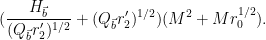
Using the bound ${s \sim Q_{\vec b}/r_1}$ , this becomes

$\displaystyle S'_{\vec b}\lessapprox M S_0 Q_{\vec b} H_{\vec b} + \sum_{r_1,r_2 \in {\mathcal S}_I: Q_{\vec b}/S_0 \ll r_1 \sim r_2 \ll yQ_{\vec b}/S_0; m_1r_1^3-m_2r_2^3 \neq 0} \sum_{s \sim Q_{\vec b}/r_1} \sum_{m_1,m_2 \sim M}$

$\displaystyle (Q_{\vec b}/r_1) (\frac{ H_{\vec b}}{[r_1,r_2]^{1/2} (Q_{\vec b}/r_1)^{1/2}} + [r_1,r_2]^{1/2} (Q_{\vec b}/r_1)^{1/2})$

$\displaystyle (m_1r_1^3 -m_2r_2^3, s)^{1/2} (r_1,r_2,m_2-m_1)^{1/2}.$

By Lemma 5 from this previous post we have

$\displaystyle \sum_{s \sim Q_{\vec b}/r_1} (m_1r_1^3 -m_2r_2^3, s) \lessapprox Q_{\vec b}/r_1$

and hence also

$\displaystyle \sum_{s \sim Q_{\vec b}/r_1} (m_1r_1^3 -m_2r_2^3, s)^{1/2} \lessapprox Q_{\vec b}/r_1$

and thus

$\displaystyle S'_{\vec b}\lessapprox M S_0 Q_{\vec b} H_{\vec b} + \sum_{r_1,r_2 \in {\mathcal S}_I: Q_{\vec b}/S_0 \ll r_1 \sim r_2 \ll yQ_{\vec b}/S_0} \sum_{m_1,m_2 \sim M} (Q_{\vec b}/r_1)^2$

$\displaystyle (\frac{ H_{\vec b}}{[r_1,r_2]^{1/2} (Q_{\vec b}/r_1)^{1/2}} + [r_1,r_2]^{1/2} (Q_{\vec b}/r_1)^{1/2}) (r_1,r_2,m_2-m_1)^{1/2}.$

Similarly, we have

$\displaystyle \sum_{m_1,m_2 \sim M: d | m_2-m_1} d^{1/2} \lessapprox \frac{M^2}{d^{1/2}} + M d^{1/2}$

for all ${d}$ , so on summing over all ${d|(r_1,r_2)}$ we have

$\displaystyle \sum_{m_1,m_2 \sim M} (r_1,r_2,m_2-m_1)^{1/2} \lessapprox M^2 + M (r_1,r_2)^{1/2}.$

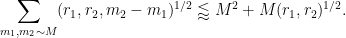
We thus have

$\displaystyle S'_{\vec b}\lessapprox M S_0 Q_{\vec b} H_{\vec b} + \sum_{r_1,r_2 \in {\mathcal S}_I: Q_{\vec b}/S_0 \ll r_1 \sim r_2 \ll yQ_{\vec b}/S_0} (Q_{\vec b}/r_1)^2$

$\displaystyle (\frac{ H_{\vec b}}{[r_1,r_2]^{1/2} (Q_{\vec b}/r_1)^{1/2}} + [r_1,r_2]^{1/2} (Q_{\vec b}/r_1)^{1/2}) (M^2 + M (r_1,r_2)^{1/2}).$

Writing ${r_0 := (r_1,r_2)}$ , ${r_1 = r_0 r'_1}$ and ${r_2 = r_0 r'_2}$ , we thus have

$\displaystyle S'_{\vec b}\lessapprox M S_0Q_{\vec b} H_{\vec b} + \sum_{r_0 \ll yQ_{\vec b}/S_0} \sum_{r'_1,r'_2 \in {\mathcal S}_I: \frac{Q_{\vec b}}{S_0 r_0} \ll r'_1 \sim r'_2 \ll \frac{yQ_{\vec b}}{S_0r_0}} (\frac{Q_{\vec b}}{r_0r'_1})^2$

$\displaystyle (\frac{ H_{\vec b}}{(Q_{\vec b} r'_2)^{1/2}} + (Q_{\vec b} r'_2)^{1/2}) (M^2 + M r_0^{1/2}).$

Performing the ${r'_2}$ summation, this becomes

$\displaystyle S'_{\vec b}\lessapprox M S_0 Q_{\vec b} H_{\vec b} + \sum_{r_0 \ll yQ_{\vec b}/S_0} \sum_{r'_1 \in {\mathcal S}_I: \frac{Q_{\vec b}}{S_0 r_0} \ll r'_1 \ll \frac{yQ_{\vec b}}{S_0r_0}} (\frac{Q_{\vec b}}{r_0})^2$

$\displaystyle (\frac{ H_{\vec b}}{Q_{\vec b}^{1/2}} (r'_1)^{-3/2} + Q_{\vec b}^{1/2} (r'_1)^{-1/2}) (M^2 + M r_0^{1/2})$

and then performing the ${r'_1}$ summation we obtain

$\displaystyle S'_{\vec b}\lessapprox M S_0 Q_{\vec b} H_{\vec b} + \sum_{r_0 \ll yQ_{\vec b}/S_0} (\frac{Q_{\vec b}}{r_0})^2$

$\displaystyle (\frac{ H_{\vec b}}{Q_{\vec b}^{1/2}} (\frac{Q_{\vec b}}{S_0 r_0})^{-1/2} + Q_{\vec b}^{1/2} (\frac{yQ_{\vec b}}{S_0 r_0})^{1/2}) (M^2 + M r_0^{1/2}).$

The net power of ${r_0}$ here is always at most ${-1}$ , so the ${r_0=1}$ term in the summation dominates:

$\displaystyle S'_{\vec b}\lessapprox M S_0 Q_{\vec b} H_{\vec b} + Q_{\vec b}^2$

$\displaystyle (\frac{ H_{\vec b}}{Q_{\vec b}^{1/2}} (\frac{Q_{\vec b}}{S_0})^{-1/2} + Q_{\vec b}^{1/2} (\frac{yQ_{\vec b}}{S_0})^{1/2}) M^2.$

We simplify this as

$\displaystyle S'_{\vec b} \lessapprox M S_0 Q_{\vec b} H_{\vec b} + M^2 H_{\vec b} Q_{\vec b} S_0^{1/2} + y^{1/2} M^2 Q_{\vec b}^3 S_0^{-1/2}. \ \ \ \ \ (43)$

To optimise this in ${S_0}$ , we select

$\displaystyle S_0 := \min( Q_{\vec b}^{4/3} M^{2/3} H_{\vec b}^{-2/3} y^{1/3}, yQ_{\vec b} ).$

(The quantity ${Q_{\vec b}^{4/3} M^{2/3} H_{\vec b}^{-2/3} y^{1/3}}$ comes from equating ${MS_0 Q_{\vec b} H_{\vec b}}$ and ${y^{1/2} M^2 Q_{\vec b}^3 S_0^{-1/2}}$ .) By construction, we have the second inequality in (40). We also claim the first inequality, since this is equivalent to

$\displaystyle H_{\vec b} \leq Q_{\vec b}^2 M y^{1/2}$

which would follow if

$\displaystyle b^{1/2} Q \frac{b}{b_1 b_2 b_3} \leq x^{1+\delta/2-4\epsilon}.$

But from (41) one has ${b^{1/2} \ll Q^{1/2}}$ and ${\frac{b}{b_1 b_2 b_3} \leq 1}$ , and the claim now follows from (36) and (13).

Inserting this value of ${S_0}$ (using ${S_0 \leq Q_{\vec b}^{4/3} M^{2/3} H_{\vec b}^{-2/3} y^{1/3}}$ for the first two terms in (43)), we conclude that

$\displaystyle S'_{\vec b} \lessapprox M^{5/3} Q_{\vec b}^{7/3} H_{\vec b}^{1/3} y^{1/3} + M^{7/3} H_{\vec b}^{2/3} Q_{\vec b}^{5/3} y^{1/6} + M^2 Q_{\vec b}^{5/2}.$

One should view the first term here as the main term. By (42), we conclude that

$\displaystyle S_{\vec b} \lessapprox M^{5/6} Q_{\vec b}^{7/6} H_{\vec b}^{2/3} y^{1/6} + M^{7/6} H_{\vec b}^{5/6} Q_{\vec b}^{5/6} y^{1/12} + M H_{\vec b}^{1/2} Q_{\vec b}^{5/4}.$

Since ${H_{\vec b} = x^{3\epsilon} H (b_1 b_2 b_3)^{-1} \leq x^{3\epsilon} H b^{-1}}$ , ${Q_{\vec b} = Q b^{-1}}$ , and ${y = x^\delta b}$ , we thus have

$\displaystyle S_{\vec b} \lessapprox x^{5\epsilon/2} b^{-1} (b_1 b_2 b_3)^{-1/2} ( M^{5/6} Q^{7/6} H^{2/3} x^{\delta/6} + M^{7/6} H^{5/6} Q^{5/6} x^{\delta/12} + M H^{1/2} Q^{5/4} ).$

From Euler products we see that

$\displaystyle \sum_{\vec b} \frac{\hbox{rad}(b_1) \hbox{rad}(b_2) \hbox{rad}(b_3)}{b^2} b^{-1} (b_1 b_2 b_3)^{-1/2} \ll 1$

and so to prove (39) it will suffice to show that

$\displaystyle M^{5/6} Q^{7/6} H^{2/3} x^{\delta/6} + M^{7/6} H^{5/6} Q^{5/6} x^{\delta/12} + M H^{1/2} Q^{5/4} \lessapprox x^{-5\epsilon} M Q^2.$

We can rewrite these conditions as upper bounds on ${H}$ :

$\displaystyle H \lessapprox x^{-\delta/4 - 15 \epsilon/2} M^{1/4} Q^{5/4}$

$\displaystyle H \lessapprox x^{-\delta/10 - 6 \epsilon} M^{-1/5} Q^{7/5}$

$\displaystyle H \lessapprox x^{-10\epsilon} Q^{3/2}.$

As ${H = Q^3 / N}$ and ${MN \sim x}$ , we can rewrite these conditions as upper bounds on ${Q}$ :

$\displaystyle Q^{7/4} \lessapprox x^{1/4-\delta/4 - 15 \epsilon/2} N^{3/4}$

$\displaystyle Q^{8/5} \lessapprox x^{-1/5-\delta/10 - 6 \epsilon} N^{6/5}$

$\displaystyle Q^{3/2} \lessapprox x^{-10\epsilon} N.$

Since ${N \gtrapprox x^{\frac{3}{2} (\frac{1}{2}+\sigma)}}$ and ${Q \lessapprox x^{1/2+2\varpi}}$ , these conditions become

$\displaystyle \frac{7}{4} (\frac{1}{2}+2\varpi) < \frac{1}{4} - \frac{\delta}{4} + \frac{3}{4} \frac{3}{2} (\frac{1}{2} + \sigma)$

$\displaystyle \frac{8}{5} (\frac{1}{2}+2\varpi) < -\frac{1}{5} - \frac{\delta}{10} + \frac{6}{5} \frac{3}{2} (\frac{1}{2} + \sigma)$

$\displaystyle \frac{3}{2} (\frac{1}{2}+2\varpi) < \frac{3}{2} (\frac{1}{2} + \sigma)$

which we may rearrange as

$\displaystyle \sigma > \frac{1}{18} + \frac{28}{9} \varpi + \frac{2}{9} \delta$

$\displaystyle \sigma > \frac{1}{18} + \frac{16}{9} \varpi + \frac{1}{18} \delta$

$\displaystyle \sigma > 2 \varpi$

but these follow from (12). The proof of Theorem 6 is complete.

94 comments

Comments feed for this article

8 July, 2013 at 12:13 am

David Roberts

(empty comment to subscribe to email updates)

8 July, 2013 at 12:37 am

Probably-clueless question here, motivated purely by aesthetics:

Clearly 2 is a gratuitously specific number :-). What happens if we replace the notion of “doubly dense divisibility” by, let’s call it, “hereditarily dense divisibility”: x is y-HDD iff either x=1 or in every interval [R/y,R] with 1 <= R <= x there is a factor of x that's also y-HDD. It seems like this is stronger than DDD but weaker than y-smoothness (but maybe intuition is deceptive here?).

8 July, 2013 at 9:21 am

Terence Tao

I think this property is equivalent to y-smoothness, since by setting R slightly less than x we see that every y-HDD number is the product of a number in (1,y] and another number which is y-HDD, and hence by induction is y-smooth. So we have a fairly continuous hierarchy of properties, from y-dense divisibility (the weakest), to double y-dense divisibility, to triple y-dense divisibility, …, all the way to hereditary y-dense divisibility or equivalently y-smoothness (the strongest property).

The sieving step can purchase us double y-dense divisibility for almost the same price as y-dense divisibility, but presumably the price keeps rising as we ask for more and more divisibility. For instance, with our current best values of $\varpi,\delta$ we can purchase double dense divsibility at $k_0=720$ (and single dense divisibility at more or less the same level), whereas smoothness requires $k_0$ to be 873 or so.

There is a chance that we will need triple or higher dense divisibility if we start iterating the van der Corput process more often than we are doing now, but thus far this seems to have been counterproductive.

8 July, 2013 at 12:55 am

Lior Silberman

Is inequality (12) reversed? Otherwise large values of $\sigma$ wouldn’t violate it.

8 July, 2013 at 9:28 am

Terence Tao

No, I think the inequalities are the right way for the Type III estimates. The parameter $\sigma$ demarcates the border between Type I and Type III; if one increases $\sigma$ , then we dump more cases into Type I (which then becomes harder to prove) but take more cases out of Type III (which becomes easier to prove). So the necessary conditions for Type I involve upper bounds on $\sigma$ while the necessary conditions for Type III involve lower bounds, which have to be balanced against each other (and with the combinatorial condition $\sigma > 1/10$ ) to get the final range of $\varpi,\delta$ . (Actually, with our current technology, the combinatorial constraint is giving a stronger lower bound than the Type III estimates, so it is not currently a critical priority to try to improve the Type III estimates further.)

8 July, 2013 at 4:57 am

Eytan Paldi

Let $P_2(x, H)$ denotes the number of consecutive prime pairs
$(p, p')$ satisfying $p > 1$ . Since it is known that
$P_2(x, 2) = O(x/ \log ^2 x)$ , the next (natural) step is to give an explicit lower bound on the growth of $P_2(x, H)$ for some $H$ , where $P_2(x,H)$ is the number of consecutive prime pairs $(p,p')$ satisfying $p < p' \leq p+H \leq x$ .

(even. $P_2(x, H) >> \log x$ should be a great advance!)

8 July, 2013 at 5:14 am

Eytan Paldi

In terms of $P_2(x, H)$ as defined above, Zhang’s theorem is equivalent to $P_2(x, H) >>1$ for some $H$ .

8 July, 2013 at 6:00 am

Lior Silberman

I haven’t followed all the details, but isn’t the argument producing an H such that, for all x large enough, there is a pair of primes at distance at most H in the interval [x,2x]? That directly gives the bound $P_2(x,H) \gg \log x$ .

8 July, 2013 at 6:30 am

Eytan Paldi

You are right of course! (it is interesting that even Bertrand’s postulate shows that Zhang’s theorem implies this seemingly stronger result.)
So perhaps the next step is to find a lower bound on the growth of P_2(x, H) as implied by the best known upper bound on the gap between consecutive primes.

8 July, 2013 at 9:34 am

Terence Tao

Dear Eytan,

You might be interested in this recent paper of Pintz at http://arxiv.org/abs/1305.6289 which discusses what results of this type one can get as consequences of Zhang’s theorem (or variants thereof). In particular, I think the bound of $P_2(x,H) \gg x /\log^{k_0} x$ can be obtained from the sieve-theoretic arguments. The arguments of Goldston, Pintz, and Yildirim at http://arxiv.org/abs/1103.5886 should in principle be able to improve this, though I don’t know if we can get the optimal $P_2(x,H) \gg x / \log^2 x$ this way. This question is a little outside of the direct scope of the Polymath8 project, but perhaps someone will look into it.

8 July, 2013 at 10:02 am

Eytan Paldi

Dear Terence, Thanks for the information ! (It seems that the conjecture that $p' = p + O(\log ^2 p)$ is sufficient to get $P_2(x, H) >>x/ \log^2 x$ )

8 July, 2013 at 11:21 am

Gergely Harcos

@Eytan: Why would $p' = p + O(\log ^2 p)$ imply $P_2(x, H) \gg x/ \log^2 x)$ ?

8 July, 2013 at 2:08 pm

Eytan Paldi

Assuming the conjecture $p_{n+1} \le p_n + C \log^2 p_n)$ for some absolute constant $C$ for each prime $p_n$ . My idea was to define the sequence $x_n, n \ge 1$ by $x_{n+1} = x_n + 3 C \log ^2 x_n$ , starting with sufficiently large $x_1$ so each interval $(x_n, x_{n+1})$ contains a pair of consecutive primes, and the number of such intervals below
$x$ is $>> x/ \log ^2 x$ , but (thanks to Gergely question) I realized that the problem is that for each fixed H, the number of H-bounded prime gaps can grow arbitrarily slower than the number of such intervals below $x$ .
So it is not clear now how to get any explicit lower bound on the growth of
$P_2(x, H)$ .

8 July, 2013 at 9:47 am

Eytan Paldi

In my previous comment (8 July, 4:57 am), the definition of $P_2(x, H)$ should be the number of consecutive prime pairs $(p, p')$ satisfying
$p < p' \le p + H \le x$ .

8 July, 2013 at 5:30 am

M Flax

In the first formula of definition (2), should log(x) be log(n)?

8 July, 2013 at 12:56 pm

Pace Nielsen

No. By convention, $\alpha$ is implicitly a function of $x$ .

8 July, 2013 at 8:57 am

Pace Nielsen

Since the current boundary is the the combinatorial bound $\sigma\geq 1/10$ , it makes sense to see what happens if we replace the approximation $N\approx x^{\frac{3}{2}(\frac{1}{2}+\sigma)}$ in the Type III computations with the weaker $N\approx x^{6\sigma}$ , which avoids the combinatorial obstacles. If we do, the three lower bounds on $\sigma$ that we obtain are

$\frac{5}{36}+\frac{7}{9}\varpi + \frac{1}{18}\delta<\sigma$

and

$\frac{1}{12}+\frac{4}{9}\varpi + \frac{1}{72}\delta<\sigma$

and

$\frac{1}{8}+\frac{1}{2}\varpi <\sigma$ .

It appears that there is room to rebalance these inequalities, but only the second one currently surpasses the $\sigma\geq 1/10$ obstacle.

It would also be interesting to rework the Type III computations but instead of working with three smooth functions use only one or two (with, respectively, $N\approx x^{2\sigma}, N\approx x^{4\sigma}$ ). We would then need to bound formulas involving $K_1,K_2$ instead of $K_3$ .

8 July, 2013 at 2:39 pm

Eytan Paldi

The pages “Dickson -Hardy-Littlewood theorems” and “Distribution of primes in smooth moduli” should be updated according to this post.

[Done, thanks for the suggestion – T.]

9 July, 2013 at 7:13 am

Eytan Paldi

More corrections:

1. In the page “Dickson-Hardy-Littlewood theorems”, in the last title MPZ should be replaced by MPZ”.
Also (to ensure that $\tilde{\theta} \le 1$ ), $\tilde{\theta}$ in the last section should be defined (as already suggested by Gergely Harcos) as the minimum between its current expression and 1.

2. In the page “Distribution of primes in smooth moduli”, in the second line MPZ” should also be mentioned. Also the definition of MPZ” should also be added as well as the definitions of $D_y$ and $D_y ^2$ .

[Corrected, thanks – T.]

9 July, 2013 at 9:50 am

Gergely Harcos

Let me clarify. Regarding Theorem 5 and its later variant of the earlier thread (https://terrytao.wordpress.com/2013/06/18/a-truncated-elementary-selberg-sieve-of-pintz/) I suggested that there was no need to redefine $\tilde\theta$ , because $G_{k_0-1,\tilde \theta}=G_{k_0-1,\min(\tilde \theta,1)}$ . The wiki page (http://michaelnielsen.org/polymath1/index.php?title=Dickson-Hardy-Littlewood_theorems) is a slightly different issue, because the Maple code there contains an upper bound for $G_{k_0-1,\tilde \theta}(0,0)$ rather than its actual value. On the other hand, this upper bound is increasing in $\tilde\theta$ (it is the antiderivative of a nonnegative function), hence if $\kappa_3$ is admissible for some $\tilde\theta>1$ , then it is admissible for the redefined $\tilde\theta:=1$ as well. This means that the Maple code worked fine in its original form (i.e. without taking the minimum of $\tilde\theta$ and $1$ ), but of course it is more efficient in its current updated form.

9 July, 2013 at 11:08 am

Eytan Paldi

Thank you! (now I understand it better.)

8 July, 2013 at 9:00 pm

Pace Nielsen

I believe that $16\delta$ in the Type I estimate bounds should be $32\delta$ .

[Sorry about this, actually the $16\delta$ is I think correct, but in the display deriving it at the bottom of Section 2, I had an $8\delta$ where there should have been a $4\delta$ instead, which I’ve now corrected. -T.]

8 July, 2013 at 11:32 pm

James Hilferty

Is all this not a little fruitless and over complicated? I have a far simpler sum, namely the Black-Scholes formula. No one has actually disproved it and for a theorem which never worked at anytime just look at all the damage it caused to the financial system. I was just recently looking at JP Morgan’s “Var” formula and they admit that there is no accurate method at predicting the price “volatility” of a future’s option and you all are trying to do something similar with your new (?) probability theorem. What do you all think?

9 July, 2013 at 7:35 am

Anonymous

I admire your imagination but deplore your ignorance.

9 July, 2013 at 9:26 am

Terence Tao

As usual, I am recording the critical numerology, i.e. the endpoint case that we currently can’t treat with our methods. Setting $\delta=0$ for simplicity, this is $\varpi = 3/280$ and $\sigma = 1/10$ . In the Heath-Brown decomposition, the enemy here is either a “Type IV” expression of the form $\psi_1 * \psi_2 * \psi_3 * \psi_4$ where $\psi_1,\psi_2,\psi_3$ are smooth and supported at scale $x^{1/5}$ and $\psi_4$ is smooth and supported at scale $x^{2/5}$ , or a “Type V” sum of the form $\psi_1 * \psi_2 * \psi_3 * \psi_4 * \psi_5$ where all of the $\psi_i$ are smooth and supported at scale $n^{1/5}$ . While it looks like the Type IV sum is treatable from the Type I method by exploiting the additional smoothness of $\beta$ in this case, it does not seem that this is available for the Type V sum, which is also far from being treatable by Type III methods.

If we attack the Type V sum by Type I methods, we factor it as $\alpha *\beta$ where $\alpha = \psi_1 * \psi_2 * \psi_3$ is supported at scale $M = x^{3/5}$ , and $\beta = \psi_4 * \psi_5$ is supported at scale $N = x^{2/5}$ . The modulus $d$ has magnitude $d \sim x^{1/2+2\varpi}$ and is factored as $d = qr$ , where $r \sim R = N = x^{2/5}$ (ignoring epsilons) and so $q \sim Q = x^{1/10 + 2\varpi}$ . After various Cauchy-Schwarz type manipulations, our task is then to show that

$|\sum_{1 \leq h \leq H} \sum_{q_1,q_2 \sim Q} \sum_n \beta(n) \beta(n+kr) \Phi_{k,r}(h,q_1,q_2;n)| \lessapprox x^{-\varepsilon} Q^2 N$

where $H \approx Q^2 R/M = x^{4\varpi}$ , and we may take $q_1,q_2$ to be coprime as the dominant case (so $q_0=1$ ). Thus we need to gain about $H \approx x^{4\varpi}$ over the trivial bound. There is also some additional averaging in the k and r parameters (the k averaging is over a negligible range, but r ranges over scales $r \sim R = x^{2/5}$ and is potentially useful) but we currently do not know how to exploit this extra averaging. The phase $\Phi_{k,r}$ is periodic with period $r q_1 q_2 \approx x^{3/5 + 4\varpi}$ .

The way we are currently treating the Type I sum, we are factoring $q_1 = s_1 t_1$ with $t_1 \approx T \approx H \approx x^{4\varpi}$ and $s_1 \approx S \approx Q/H \approx x^{1/10 - 2\varpi}$ . After Cauchy-Schwarz, we are reduced to showing that

$\sum_{1 \leq h,\tilde h \leq H; t_1,\tilde t_1 \sim T; s_1 \sim S; q_2 \sim Q}$

$|\sum_n \psi_N(n) \Phi(h, s_1 t_1, q_2; n) \overline{ \Phi(\tilde h, s_1 \tilde t_1, q_2; n) } |$

$\lessapprox x^{-\varepsilon} TSQN,$

thus we need to save a factor of $H^{-2} = x^{-8\varpi}$ over the trivial bound. Thus, on average, we need to obtain an exponential sum estimate of the form

$|\sum_n \psi_N(n) \Psi_q(n)| \lessapprox x^{-8\varpi-\varepsilon} N$

where $\Psi_q$ is an explicit but slightly messy phase of period $q = r s_1 t_1 \tilde t_1 q_2 \approx x^{3/5+8\varpi}$ . With the particular choice of $\varpi = 3/280$ , we have $N \sim q^{7/12}$ and $x^{8 \varpi} \sim q^{1/8}$ , so our objective is to prove something like

$|\sum_{n \sim q^{7/12}} \Psi_q(n)| \lessapprox q^{11/24 - \varepsilon}$

for an “average” phase $\Psi_q$ of period $q$ (as a zeroth approximation, think of the model case $\Psi_q(n) = e_q(c/n)$ where $c$ ranges over a shortish interval, say of length $x^{8\varpi} \approx q^{1/8}$ ). This is currently being treated by the van der Corput estimate, which roughly has the shape

$|\sum_{n \sim N} \Psi_q(n)| \lessapprox N^{1/2} q^{1/6}$ (*)

which doesn’t save the epsilon, and is ultimately why we just barely fail to make $\varpi$ reach $3/280$ . So the basic challenge is to do better than (*) when $N \sim q^{7/12}$ , possibly after exploiting the additional averaging in the $k, r, h, \tilde h, t_1, \tilde t_1, s_1, q_2$ parameters that are available. But these parameters are hard to exploit: the k averaging is negligible, the $r,t_1,s_1,q_2$ averages are substantial but affect the modulus which is bad, leaving only the $h,\tilde h$ averaging which looks promising but is only over a fairly short range. A model problem would be to obtain a bound of the form

$|\sum_{c \sim q^{1/8}} \sum_{n \sim q^{7/12}} e_q( c/n )| \lessapprox q^{7/12 - \varepsilon}$

for a “typical” sufficiently smooth modulus $q$ , whatever “typical” means. (Here we are implicitly using smooth cutoffs where necessary, and adopting the convention that $e_q(c/n)$ vanishes when $n$ is not coprime to $q$ .)

9 July, 2013 at 10:40 am

Terence Tao

By chance I happened to attend a nice talk by Igor Shparlinski while at Budapest in which he gave a nice summary of the start of the art on how to estimate multidimensional incomplete exponential sums (though he focused primarily on the prime modulus case rather than the smooth modulus case). In addition to the standard technique of completion of sums, he also mentioned Vinogradov-type techniques (which are traditionally used to estimate exponential sums over the integers, e.g. for Waring’s problem or in bounding the zeta function, but can also give non-trivial results in finite fields), as well as the sum-product methods of Bourgain and co-authors (but this requires a lot of multiplicative structure), and also the Burgess type arguments (again this requires some sort of multiplicativity in the phase though).

Another route is to develop the q-van der Corput theory more fully, basically replicating the theory of exponent pairs in the q-setting. There are some exponent pairs that are known that are not obtainable from the standard A- and B- processes (e.g. the work of Huxley and Watt). These may end up being a bit complicated to execute though (if we do too many fancy manipulations, the dependence on $\delta$ is eventually going to hurt us; also, the Deligne-type exponential sum we will need to control at the end gets more and more complicated, though perhaps there is only a finite amount of algebraic geometry verification to be done for each specific application of this machinery).

One route that looks moderately promising to me is to try to combine the van der Corput A-process that we are currently using with the additional averaging in auxiliary parameters such as $h,h'$ that we are currently unable to exploit (I called this a “Level 5” Type I estimate on the wiki). This should attenuate the diagonal contribution which should allow for some rebalancing of parameters that takes some of the load off of the off-diagonal contribution. (This trick already was used to good effect on the Type III sums.) I’ve tried to do this a few times in the last few days, but the problem has always been that the parameters being averaged over are over a shorter range than the difference $q_1$ that one is Weyl differencing over so no additional gain could be extracted, but I did not exhaust all the possible permutations of this strategy.

ADDED LATER: I forgot to add automorphic forms techniques (or “Kloostermania”) as a possible further technique which can exploit averaging in the modulus although once one moves away from the model problem and starts considering more realistic sums such as $\sum_c \sum_n e_q( a_q c / n )$ where $a_q$ varies with $q$ in a manner consistent with the Chinese remainder theorem, my understanding is that these methods become significantly more difficult to deploy.

9 July, 2013 at 10:52 am

Pace Nielsen

Dear Terry,

Thank you for this analysis. I’ll try to absorb it more fully over the next week. In the meantime I did have a few questions (some perhaps easier to answer than others).

1. I’m a little weak on when it is allowable to use the Linnik decomposition rather than the Heath-Brown decomposition. Assuming that we can use the Linnik decomp., is there any extra information we gain that helps in these analyses? For instance, do we gain any insight into the scales involved in the coefficient sequences?

2. In your computations above, you take $\beta=\psi_4\ast \psi_5$ . Another option would be to take $\beta=\psi_5$ and try to take advantage of the smoothness of $\beta$ . Does the smoothness (and thus avoidance of an extra Cauchy-Schwarz) make up for the smaller scale size? Or is this just a pipe dream?

3. Perhaps a better way to take advantage of the smoothness would instead be to modify the Type III computations from $\alpha\ast \psi_1\ast \psi_2\ast \psi_3$ to $\alpha \ast \psi_1\ast \psi_2$ or $\alpha \ast \psi_1$ (with $\psi_i$ of scale $N_i\sim x^{2\sigma}$ ). This would replace bounds on $K_3$ with needing bounds on $K_2, K_1$ , which seem to be much more controllable. (Again, this might be a pipe dream.)

Best wishes,
Pace

9 July, 2013 at 7:54 pm

Terence Tao

Dear Pace,

1. Morally speaking the Linnik decomposition should work in these arguments, but it has infinitely many terms and there is basically no hope of controlling sums involving the divisor function $\tau'_k$ with a really good dependence on k. Note for instance that $\sum_{n \leq x} \tau'_k(n) \mu(n)$ is (conjecturally on the Mobius pseudorandomness conjecture) believed to be $o(x)$ for any fixed $k$ (with the decay rate being highly non-uniform in $k$ ), while $\sum_{n \leq x} \Lambda(n) \mu(n)$ is certainly not $o(x)$ , so one can’t hope to use Linnik to get good estimates for $\Lambda$ from good estimates for $\tau'_k$ .

2. Let’s do a quick computation. If one halts the Type I argument before the final Cauchy-Schwarz, the objective in the critical case is to obtain an estimate roughly of the form

$|\sum_n \beta(n) \beta(n+kr) \Phi_q(n)| \lessapprox x^{-\varepsilon} H^{-1} N$

for some phase $\Phi_q(n)$ of period $q = r q_1 q_2 \approx x^{1/2+\sigma+4\varpi}$ , where $H \approx x^{4\varpi}$ . If $\beta$ is smooth, one can use the completion of sums bound

$|\sum_n \beta(n) \beta(n+kr) \Phi_q(n)| \lessapprox q^{1/2}$

which suggests the constraint

$\frac{1}{2} (\frac{1}{2} + \sigma + 4 \varpi) < - 4\varpi + \frac{1}{2} - \sigma$

which rearranges to

$6 \sigma + 24 \varpi < 1.$

If we instead use the van der Corput bound

$|\sum_n \beta(n) \beta(n+kr) \Phi_q(n)| \lessapprox N^{1/2} q^{1/6}$

then we are led to the constraint

$\frac{1}{2} (\frac{1}{2}-\sigma) + \frac{1}{6} (\frac{1}{2} + \sigma + 4 \varpi) < - 4\varpi + \frac{1}{2} - \sigma$

which becomes

$4 \sigma + 28 \varpi < 1.$

This is a bit better than the current Type I constraint of $4\sigma + 56 \varpi < 1$ , with $\varpi = 3/280$ , it allows us to take $\sigma$ as large as $7/40 = 0.175$ when $\beta$ is smooth, so we can basically handle any configuration $(t_1,\ldots,t_n)$ of exponents with $t_1 > 13/40 = 0.325$ . That’s not bad – it should dispose of most of the “Type IV” type sums we will encounter – but still quite far from dealing with the tuple $(1/5,1/5,1/5,1/5,1/5)$ which would basically require stretching $\sigma$ to be as large as $3/10$ .

If we apply the next iteration of van der Corput, this gives

$|\sum_n \beta(n) \beta(n+kr) \Phi_q(n)| \lessapprox N^{5/7} q^{1/14}$

leading to the constraint

$\frac{5}{7} (\frac{1}{2}-\sigma) + \frac{1}{14} (\frac{1}{2} + \sigma + 4 \varpi) < - 4\varpi + \frac{1}{2} - \sigma$

which rearranges as

$\frac{10}{3} \sigma + 40 \varpi < 1$

which, at $\varpi = 3/280$ , gets $\sigma$ as large as $6/35 = 0.171\ldots$ , which is actually worse than what we got with just one van der Corput (which is consistent with the other times that we have tried iterated van der Corput, the gain in the $\sigma$ aspect is generally outweighed by the loss in the $\varpi$ aspect). So we’re not making much progress here towards stretching the Type I sums all the way to the $\sigma=3/10$ case when $\beta$ is smooth.

One last numerology check: if we assume the most optimistic exponential sum bound (the Hooley conjecture)

$|\sum_n \beta(n) \beta(n+kr) \Phi_q(n)| \lessapprox N^{1/2},$

one gets

$2\sigma + 16 \varpi < 1$

which clears the bar with room to spare ( $\sigma$ can now be as large as $29/70 = 0.4143\ldots$ ). So there is hope, but it does require quite strong exponential sum estimates.

3. I haven’t given this a shot yet, but I’ll take a look at the suggestion.

10 July, 2013 at 10:15 am

Pace Nielsen

Dear Terry,

Thank you for working this out. It appears that I wasn’t conveying myself well, since my question #2 was about a lower bound on $\sigma$ , not upper bounds. However, your answer was still extremely helpful for me, and hopefully will help me explain my idea a bit better.

For simplicity I’m going to ignore all the $\delta$ ‘s and $\epsilon$ ‘s.

As you know, the combinatorial data gives a natural meeting place between the Type I/II and Type III sums, which can be thought of as given, respectively, by upper and lower bounds on $\sigma$ . The Type III sums arise from consideration of how many smooth sequences have scales somewhere in the range $[x^{2\sigma},x^{1/2-\sigma}]$ . If there are too few (or too many) such sequences (and $1/10 <\sigma$ ), then we can reduce to the Type I/II bounds. On the other hand, if there are exactly three sequences in this range, we can then either again reduce to the Type I/II bounds, or we have that the product of the three scales is at least $x^{3/2(1/2+\sigma)}$ which we call the Type III case.

My idea is to forget about some of this information in exchange for weaker combinatorial restrictions. So, for example, when we are in the Type III situation I forget about the fact that there are three smooth sequences in the range $[x^{2\sigma},x^{1/2-\sigma}]$ for which the product of the scales is fairly large, and instead only retain the information that there is a single smooth sequence in the range. This is clearly going to lead to inequalities worse than the usual Type III bounds, but as the current restriction occurs between the Type I bounds and $\sigma=1/10$ , this might not be too bad.

So, now let's work through the numerology. We have $N\approx x^{2\sigma}$ . Similarly, $R\approx N \approx x^{2\sigma}$ since we are ignoring $\delta$ . We also have $H\approx Q^{2}R/M \approx (QN)^{2}/x$ , where $x^{1/2}\lessapprox QN\lessapprox x^{1/2+2\varpi}$ . Finally, $q=rq_1q_2\approx (QN)^{2}/N$ . Now let's consider the four types of bounds from your post.

————**Completion of sums**—————

We need $q^{1/2} \lessapprox N/H$ . This leads to $(QN)^{3} \lessapprox xN^{3/2}$ . Hence

$\frac{1}{6}+2\varpi < \sigma$ .

This, in conjunction with the given Type I bound, yields $\varpi < 1/192$ which is worse than what we normally get.

————–**van der Corput once**—————-

We need $N^{1/2}q^{1/6} \lessapprox N/H$ . This leads to $(QN)^{2+1/3} \lessapprox xN^{1-1/2+1/6}$ . Hence

$\frac{1}{8} + \frac{3}{2}\varpi < \sigma$ .

This, in conjunction with the given Type I bound, yields $\varpi < 1/124$ .

—————–**van der Corput twice**—————-

We need $N^{5/7}q^{1/14} \lessapprox N/H$ . This leads to $(QN)^{2+1/7} \lessapprox xN^{1-5/7+1/14}$ . Hence

$\frac{1}{10}+6\varpi < \sigma$ .

This, in conjunction with the given Type I bound, yields $\varpi < 3/400$ , which is worse than the single van der Corput.

Notice further that in all three cases we never surpass the $1/10<\sigma$ bound.

—————-**Hooley Conjecture**———————

We need $N^{1/2} \lessapprox N/H$ . This leads to $(QN)^{2} \lessapprox xN^{1-1/2}$ . Hence

$4\varpi <\sigma$ .

In this case, it appears that we can actually remove all of the Type I considerations and reduce to the Type II sums!

10 July, 2013 at 11:57 am

Terence Tao

In case you’re interested, the general form of the van der Corput estimate (assuming as much smoothness as needed) is

$|\sum_n \psi_N(n) \Phi_q(n)| \lessapprox N^{1 - \frac{k+1}{2^{k+2}-2}} q^{1 / (2^{k+2} - 2)}$

so $q^{1/2}$ for $k=0$ (completion of sums), $N^{1/2} q^{1/6}$ for $k=1$ (single van der Corput), $N^{5/7} q^{1/14}$ for $k=2$ (double van der Corput), $N^{5/6} q^{1/30}$ for $k=3$ , and so forth. I believe one would eventually push $\sigma$ down as low as desired by continually iterating van der Corput, but it becomes exponentially expensive in $\varpi$ to do so, so unfortunately it is not a net win. (However if one just wants to prove Zhang’s theorem and don’t care how small $\varpi$ (or $\delta$ ) has to be, I think we now have the technology to do so entirely using the Type II argument, and we could even replace the completion of sums bound $q^{1/2}$ by the weaker, but more elementary, Kloosterman bound of $q^{3/4}$ that avoids the Weil conjectures completely.)

10 July, 2013 at 3:11 pm

Terence Tao

I played around a little with item 3, i.e. modifying the Type III computations to deal with $\alpha * \psi_1 * \psi_2$ or $\alpha * \psi_1$ instead of $\alpha * \psi_1 * \psi_2 * \psi_3$ . This is like asking for averaged distribution results for the trivial divisor function $\tau_1 = 1$ or the classical divisor function $\tau_2(n) = \sum_{n_1 n_2 = n} 1$ rather than the third order divisor function $\tau_3(n) = \sum_{n_1 n_2 n_3 = n} 1$ . It turns out that while the distribution results for the former functions are indeed better than the latter, this is more than compensated by the fact that a much smaller portion of the total convolution is actually coming from the divisor function in these cases, so it doesn’t look like a win.

To illustrate what is going on let us revert to “Level 3” Type III estimates that do not exploit the alpha averaging. Fouvry, Kowalski, Michel, and Nelson showed that $\tau_3$ has a level of distribution of 4/7 for smooth moduli, which roughly speaking means that they have good control on $\sum_{n \leq N: n=a\ (q)} \tau_3(n)$ on average for $q \lessapprox N^{4/7}$ . This allows one to get good distribution results for $\alpha * \psi_1 * \psi_2 * \psi_3$ for moduli $q \lessapprox x^{1/2+2\varpi}$ , where each $\psi_i$ is supported at scale $x^{t_i}$ , provided that

$\frac{1}{2} + 2 \varpi < \frac{4}{7} (t_1 + t_2 + t_3).$

Now suppose we work instead with $\tau_2$ . Here the classical result of Linnik and Selberg is that the level of distribution is at least 2/3. (Sketch of proof: one basically needs to estimate $\sum_{n \sim N} \sum_{m \sim M} 1_{nm = a\ (q)}$ to accuracy $o( NM/q )$ when $q = o( (NM)^{2/3} )$ . Assuming $N,M = o(q)$ , we can perform Fourier summation and reduce to estimating $\sum_{h = O(q/N)} \sum_{k = O( q/M) } \sqrt{q} K_2( \frac{ahk}{n}; q )$ to accuracy $o( \frac{q}{N} \frac{q}{M} \frac{NM}{q} ) = o(q)$ , where $K_2$ is the normalised Kloosterman sum

$K_2(a;q) = \frac{1}{\sqrt{q}} \sum_{xy = a\ (q)} e_q( x + y).$

If one then uses the Weyl bound $|K_2| \lessapprox 1$ (ignoring the zero frequency contribution $a=b=0$ ), we obtain the desired claim.) For smooth moduli, Fouvry and Iwaniec (and Katz) improved the 2/3 slightly to 2/3+1/48, and perhaps with Zhang's new arguments one can push this a bit further, but let's work with the 2/3 number for now. This gives good estimates for $\alpha * \psi_1 * \psi_2$ when

$\frac{1}{2} + 2 \varpi < \frac{2}{3} (t_1 + t_2).$

This constraint is better in that the 4/7 is improved to a 2/3, but worse in that we are only summing two of the $t_i$ instead of one. In the model case $t_1=t_2=t_3$ we end up significantly worse off if we try to use this estimate.

Finally, if we work with $\tau_1$ , this trivially has level of distribution 1, so we obtain a good estimate for $\alpha * \psi_1$ when

$\frac{1}{2} + 2\varpi < t_1.$

This is the Type 0 estimate that we are already using. Again, the 4/7 or 2/3 factor has been improved to 1, but at the cost of now only using one of the $t_i$ , so this is not a win in the cases we need the most badly.

Finally, for $\tau_4$ we do not have level of distribution results better than 1/2 for smooth moduli (though in principle the Type I/II/III estimates we have should give us something which is at least as good as the estimates we have for MPZ, and perhaps a little bit better because the pesky Type V sums don’t appear for $\tau_4$ – actually, it might be worth having a look to see what numerology we can get for $\tau_4$ , as this may offer a benchmark as to what to hope to get for $\Lambda$ ), so we only get

$\frac{1}{2} + 2 \varpi < \frac{1}{2} (t_1+t_2+t_3+t_4)$

which is in fact never satisfied for any positive $\varpi$ .

The numerology changes a bit if we use the latest Type III estimates but I think the general picture is more or less the same.

10 July, 2013 at 4:41 pm

Pace Nielsen

Thanks once again for answering my questions. What seems surprising to me is how badly the constants work out in the $t_1=t_2=t_3=1/5$ case. Perhaps more surprising to me is that even though the Type III summation techniques have been optimized to improve the lower bound on $\sigma$ , we seem to do better using the techniques from the Type I case when we are restricted to two sequences. That is, when trying to deal with sums involving $\alpha\ast \psi$ with $\psi$ smooth of scale $N=x^{2\sigma}$ , we get better bounds trivially modifying the Type I techniques rather than using the techniques for Type III. Unfortunately, even if it were the case that some methods from the Type I analysis made the Type III analysis turn out better, that isn’t the current point of conflict.

Thank you for your very clear analysis. It appears that to make any headway on the Type V sums, we would need to improve the level of distribution for $K_4$ quite a bit (or to get Hooley’s conjecture and skip it all).

9 July, 2013 at 11:29 pm

Sniffnoy

Just a question from an interested onlooker: Everything since H=12006 has been marked “?”. What part of H=5414 is still unconfirmed?

10 July, 2013 at 8:26 am

Terence Tao

Basically, these later bounds rely on the Type I, II and III estimates described first in a number of scattered blog comments, and then finally compiled in one place in this blog post. So far, none of the other participants of the project have confirmed these estimates (they are somewhat lengthy, and there are a number of places where an arithmetic error could occur; I myself found a few minor ones when converting the comments to the blog format), but this will presumably happen eventually. (It’s not as if we are racing against time here.)

10 July, 2013 at 5:00 pm

Terence Tao

I think I figured out a way (in principle, at least, subject to the verification of some Deligne-level exponential sum estimates) to improve the van der Corput estimate

$|\sum_n \psi_N(n) \Phi_q(n)| \lessapprox N^{1/2} q^{1/6}$

for smooth functions $\psi_N$ at some scale $N \ll q$ and some reasonable phase $\Phi_q(n)$ (e.g. the Kloosterman phase $\Phi_q(n) = e_q(c/n)$ ) periodic with a smooth period $q$ , very slightly to

$|\sum_n \psi_N(n) \Phi_q(n)| \lessapprox N^{1/2} q^{2/13}$

if one is allowed to do some averaging in the q aspect, and if one ignores the role of $\delta$ . As far as the Type I sums are concerned, this would improve the constraint

$\frac{1}{2} (\frac{1}{2}-\sigma) + \frac{1}{6} ( \frac{1}{2} + \sigma + 8\varpi ) < -8\varpi + \frac{1}{2}-\sigma$

(or equivalently, $56\varpi + 4 \sigma < 1$ ) to

$\frac{1}{2} (\frac{1}{2}-\sigma) + \frac{2}{13} ( \frac{1}{2} + \sigma + 8\varpi ) < -8\varpi + \frac{1}{2}-\sigma$

(or equivalently $\frac{160}{3} \varpi + \frac{34}{9} \sigma < 1$ ). Playing this against $\sigma > 1/10$ , this suggests that we can improve $\varpi$ from $3/280 \approx 0.0107$ to $7/600 \approx 0.0117$ – not much, but better than nothing. (Using xfxie’s table at http://www.cs.cmu.edu/~xfxie/project/admissible/k0table.html , this should correspond to $k_0$ somewhere near 630, which by the prime tuples page at http://math.mit.edu/~primegaps/ suggests a value of $H$ somewhere near 4660. But this is an extremely rough back-of-the-envelope calculation.)

To explain the strategy, let me make the general remark that much of the game here is trying to estimate averaged exponential sums such as

$\sum_{h_1 = O(H_1)} \alpha_1(h_1) \ldots \sum_{h_k = O(H_k)} \alpha_k(h_k) \Phi_q(h_1,\ldots,h_k)$

where the $\alpha_1,\ldots,\alpha_k$ are various weights at various scales $H_1,\ldots,H_k$ and $\Phi$ is some explicit algebraic phase depending on $h_1,\ldots,h_k$ ; also the modulus $q$ is also allowed to depend on one or more of the $h_1,\ldots,h_k$ parameters. The various averages $\sum_i \alpha_i(h_i)$ can be informally divided into various types:

* “smooth” averages (in which $\alpha_i$ is smooth) and “rough” averages (in which $\alpha_i$ has no smoothness).

* “long” averages (in which $H_i$ is large) and “short” averages (in which $H_i$ is small).

* “non-modulus-altering” averages (in which $q$ does not depend on $h_i$ ) and “modulus-altering” averages (in which $q$ does depend on $h_i$ ).

Basically, we want to have smooth long non-modulus-altering averages around, because there are a lot of techniques available (e.g. completion of sums) for exploiting such averaging. In contrast, averages that are rough, short, and/or modulus-altering are not easy to exploit directly and so often just have to be discarded through the triangle inequality. However, the Cauchy-Schwarz inequality and its variants (e.g. Weyl differencing, dispersion method, or Holder’s inequality) can often be used to convert a “bad” average to a “good” average, albeit at the cost of “square-rooting” any gain one gets (and often the modulus $q$ grows a little bit after one applies Cauchy-Schwarz). So the game is to use Cauchy-Schwarz as sparingly as possible to extract one or more “good” averages that one can then squeeze some cancellation out of (which, in all of our arguments so far, is only obtainable by using completion of sums combined with the Weil conjectures).

The point is that when one applies the van der Corput method once, there is a moderately long smooth average in a parameter $d_1$ which manages to not alter the modulus. After using Fourier inversion to deal with another long smooth average, we can then deal with the moderately long smooth average by a second van der Corput. (In principle one could keep iterating this procedure, but it is already rather complicated as it is so I won’t try to do so here.)

OK, to the details. We will study the averaged sum

${\bf E}_{q \sim Q} |\sum_n \psi_N(n) \Phi_q(n)|.$

We factor $q = d_1 d_2$ where $d_1 \sim D_1$ , $d_2 \sim D_2$ , and $D_1 D_2 = Q$ is to be optimised in later, though we assume we are in the regime $D_1 \ll N \ll D_2$ which is the regime of interest when applying van der Corput. We throw away the $d_2$ averaging and just average in $d_1$ , thus we need to bound

${\bf E}_{d_1 \sim D_1} |\sum_n \psi_N(n) \Phi_{d_1 d_2}(n)|.$

for a given $d_2 \sim D_2$ .

We perform Weyl differencing in the $d_1$ direction and end up staring at

${\bf E}_{d_1 \sim D_1} |{\bf E}_{k = o(N/D_1)} \sum_n \psi_N(n+kd_1) \Phi_{d_1 d_2}(n+kd_1) |.$

Pulling out the n summation from the absolute values and then applying Cauchy-Schwarz, we can bound this by

$N^{1/2} ( {\bf E}_{d_1 \sim D_1} \sum_n {\bf E}_{k,k' = o(N/D_1)} \psi_N(n+kd_1) \psi_N(n+k'd_1)$
$\Phi_{d_1 d_2}(n+kd_1) \overline{\Phi_{d_1 d_2}(n+k'd_1)} )^{1/2}.$

The diagonal term $k=k'$ contributes $O( N^{1/2} D_1^{1/2} )$ . For the off-diagonal terms, we crucially note (as in previous applications of van der Corput) that the $d_1$ component of the phases cancel, and the phase $\Phi_{d_1 d_2}(n+kd_1) \overline{\Phi_{d_1 d_2}(n+k'd_1)}$ collapses to something like $\tilde \Phi_{d_2}( k, k', d_1, n )$ , so we are now looking at

$N^{1/2} | {\bf E}_{d_1 \sim D_1} \sum_n {\bf E}_{k,k' = o(N/D_1); k \neq k'} \tilde \psi_N(n) \tilde \Phi_{d_2}(k,k',d_1,n) |^{1/2}.$

for the off-diagonal contribution, where $\tilde \psi_N$ is some smooth cutoff function whose exact form is not too important here. If we estimate this by completion of sums, we get an additional term of $N^{1/2} D_2^{1/4}$ , giving the van der Corput bound of $O( N^{1/2} D_1^{1/2} + N^{1/2} D_2^{1/4} )$ which optimises to $O( N^{1/2} q^{1/6} )$ as before. To do better than this, we first deal with the n summation by Fourier inversion, rewriting the above as something like

$N^{1/2} | {\bf E}_{d_1 \sim D_1} {\bf E}_{h = O( D_2/N)} {\bf E}_{k,k' = o(N/D_1); k \neq k'} D_2^{1/2} K( h, k, k', d_1; d_2) |^{1/2}$

where $K$ is the Kloosterman-type sum

$K(h,k,k',d_1; d_2) := \frac{1}{\sqrt{d_2}} \sum_{n \in {\bf Z}/d_2{\bf Z}} \tilde \Phi_{d_2}(k,k',d_1,n) e_{d_2}(hn).$

The point is that the $d_1$ summation is a moderately long smooth average (of length vaguely comparable to $d_2^{1/2}$ or so) that does not affect the modulus of $K(h,k,k',d_1;d_2)$ , and so (assuming certain Deligne-level estimates are OK) we expect a van der Corput bound of the form

$|\sum_{d_1 \sim D_1} K( h, k, k', d_1; d_2)| \lessapprox D_1^{1/2} d_2^{1/6}$

which if one does the arithmetic gives a bound of $N^{1/2} D_2^{1/3} D_1^{-1/4}$ for the off-diagonal terms. We have thus bounded the original exponential sum by

$O( N^{1/2} D_1^{1/2} + N^{1/2} D_2^{1/3} D_1^{-1/4} )$

which optimises to $N^{1/2} Q^{2/13}$ as claimed by setting $D_1 := Q^{4/13}$ and $D_2 := Q^{9/13}$ .

10 July, 2013 at 5:37 pm

Anonymous

Terry, Let’s do a trade, I go to ucla to learn math from you, you learn Cantonese from me, OK?

10 July, 2013 at 7:38 pm

Pace Nielsen

What prevents one from starting with a rough sequence, and then introducing a smooth sequence at the Cauchy-Schwarz step, as has been done in the past? (I initially thought there might be problems as now $\psi_N$ depends not only on $n$ but also $k,d_1$ . But if that were the issue, wouldn’t it also cause problems in the Fourier inversion step as well? I’m probably just missing something simple here.)

10 July, 2013 at 8:29 pm

Terence Tao

Yes, one can use Cauchy-Schwarz to convert all sorts of rough sequences to smooth sequences, but it can cause some of the other averages to be duplicated, and more importantly it square roots the gain one gets at the end of the day (or equivalently, it doubles the amount of gain one now has to produce to meet one’s original objectives). For instance, if one had to gain $x^{-4\varpi}$ over the trivial bound for an averaged exponential sum involving a rough sequence and then used Cauchy-Schwarz to make the rough sequence smooth, one would now have to gain $x^{-8\varpi}$ over the trivial bound (this is how the Type I and Type II arguments eliminate the rough sequence $\beta(n) \beta(n+kr)$ ).

In the van der Corput analysis above, it turns out that all the relevant sequences are already smooth; we need Cauchy-Schwarz to perform Weyl differencing but not to eliminate rough sequences (well actually there is a rough sequence implicit in the $d_1$ summation (which lies outside the absolute values) that is eliminated by the Cauchy-Schwarz that performs the Weyl differencing, so the Cauchy-Schwarz is actually doing double duty here).

16 July, 2013 at 8:19 am

Philippe Michel

I think, the required Deligne type estimates are valid here: the Kloosterman type sum that occurs $K(h)$ say (the Fourier transform of a fraction looking like $x\rightarrow 1/(x-k_1)-1/(x-k_2)$ for $k_1\not=k_2$ ) is the Frobenius trace function of a sheaf which has a singularity at $0$ .

Now the VdC method amounts to knowing whether some non-trivial additive shift of K can correlate with K times a(ny) additive character (then, in absence of correlation, Deligne bootstraps this to square root cancellation). This is equivalent to deciding whether or not the additive shift of the sheaf underlying $K$ is geometrically isomorphic to the tensor product of itself with the trivial or any Artin-Schreier sheaf. In particular these isomorphic sheaves would have the same singularities on the affine line (since additive translation fixes infinity). The Artin-Schreier sheaf has no singularities on the affine line (hence cannot “destroy” any of the affine singularities of $K$ in the tensor product), that means that the set of affine singularities of $K$ (which is non-empty) would have to be invariant under non-trivial additive translation and in particular would cover the whole finite field which is not possible (if $p$ is large enough). There are probably other arguments possible but that one is fairly general.

These sort of things will be explained in more details in my lectures tomorrow.

16 July, 2013 at 10:55 am

Terence Tao

Great! Looking forward to your lectures (at Caltech) tomorrow; this sheaf-based perspective to Deligne type estimates does indeed seem to be very well suited for analytic number theory, as all the basic operations on phases or Kloosterman sums on finite fields (e.g. Weyl differencing, pointwise multiplication, Fourier transforms, or computing correlations) seem to have natural geometric counterparts on the associated sheaves. Will definitely be taking notes :)

17 July, 2013 at 6:49 pm

Terence Tao

Dear Philippe,

After your very nice lectures (I now understand the role of l-adic sheaves a lot better now!) I tried to flesh out the Deligne-level estimates needed for the multiple van der Corput, but unfortunately I found that the sheaf Fourier transform of Deligne, Laumon, and Katz isn’t quite appropriate for the correlation sum needed, because I need the sheaf to run over a different variable than the Fourier variable.

Let me explain with the model problem of estimating an averaged incomplete Kloosterman sum

$\sum_{q \sim Q}|\sum_{n \sim N} e_q( a / n )|$

(being vague about smooth cutoffs etc.), and with $q$ smooth. We factor $q = d_1 d_2$ for some suitable $d_1,d_2$ of a certain magnitude $D_1,D_2$ and throw away the $d_2$ averaging, leaving us with

$\sum_{d_1 \sim D_1} |\sum_{n \sim N} e_{d_1 d_2}( a / n )|.$

For the inner sum we perform the q-van der Corput A-process in the $d_1$ direction, which leaves us with the task of bounding things like

$\displaystyle |\sum_{d_1 \sim D_1} \sum_{n \sim N} e_{d_1 d_2}( \frac{a}{n+kd_1} - \frac{a}{n} )|$

for some non-zero $k$ (one could conceivably try to exploit averaging in the $k$ parameter, but I will not attempt this here). As usual, the modulus of the phase collapses from $d_1 d_2$ to $d_2$ (which is the whole point of the q-van der Corput process):

$\displaystyle |\sum_{d_1 \sim D_1} \sum_{n \sim N} e_{d_2}( \frac{ka}{n(n+kd_1)})|.$

Now we perform completion of sums in the n variable and end up with things like

$\displaystyle |\sum_{d_1 \sim D_1} \sum_{n \in {\bf Z}/d_2} e_{d_2}( \frac{ka}{n(n+kd_1)} + hn)|$

for various $h$ (again, we will not attempt to exploit averaging in $h$ , it is quite a short average in practice). So we need to control something like

$\sum_{d_1 \sim D_1} K( ka, kd_1, h; d_2 )$

where $K$ is the Kloosterman-type sum

$\displaystyle K( a, b, h; d_2 ) := \frac{1}{\sqrt{d_2}} \sum_{n \in {\bf Z}/d_2} e_{d_2}( \frac{a}{n(n+b)} + hn ).$

Now, the Deligne-Laumon-Katz theorem lets us express $K$ as the trace of a Frobenius of a lisse sheaf in the h variable, but unfortunately that’s the wrong variable; we instead need a sheaf interpretation of $K$ in the b variable. That’s not obviously a Fourier transform, so DLK does not directly apply. It’s still the pushforward of a two-dimensional sheaf, though, so in principle one can still view it as a one-dimensional sheaf (though it may be a bit harder to track the singularities – presumably Laumon’s sheaf-theoretic stationary phase still applies though? Also, it may be trickier to maintain geometric irreducibility in this variable, since we don’t have the Plancherel trick any more).

17 July, 2013 at 10:29 pm

Philippe Michel

Oh I see; sorry, I took the wrong variable; thanks for correcting. I will look at the right problem now.

18 July, 2013 at 2:54 am

Gergely Harcos

Dear Philippe and Terry, it would be nice and useful to have a brief account of the l-adic techniques and their relation to older techniques (or alternately a transcript/recording/notes of Philippe’s lectures) on this blog.

18 July, 2013 at 8:42 am

Terence Tao

I’ll try to write something over the coming days. Philippe, Emmanuel, and Etienne are planning a monograph on this topic but that will probably take a bit longer :) [But Chapter 11 of Iwaniec-Kowalski already has a pretty good summary.]

18 July, 2013 at 2:15 pm

Philippe Michel

I think that being irreducible may not be too much an issue: given $K$ some trace function associated to some sheaf $KK$ the VdC method requires that for all but a bounded number of $l$ , $x \to K(x+l)$ does not correlate with $K(x)\psi(x)$ for any additive character $\psi$ . If $KK$ is irreducible this would work for all non-zero $l$ (provided $p$ is large compared to the conductor that $KK$ satisfy some mild additional condition like having a singularity on the affine line or large enough Swan conductor at $\infty$ , $>2 ?$ -the later to avoid thing like quadratic phases-).

If there are more than one irreducible component (each one satisfying the assumptions above) then it seem that the number of bad $l$ might increase but by a bounded amount only. That concerns of course the weight 0 part and if the sheaf mixed of weight $\leq 0$ the contribution from the negative weight part can be bounded trivially. So maybe there is a relatively soft proof of this form of VdC for general $K$ : of course one needs to know a bit about that specific sheaf and especially its weight 0 part but maybe not as much as one would know if it were a Fourier transforms.

That is an interesting question !

18 July, 2013 at 2:43 pm

Terence Tao

I think it may be convenient to decompose $K$ into irreducible components before applying the vdC method (this may require some uniformity of the decomposition (e.g. uniform bounds on the conductor of the components) with respect to all the various primes p dividing the modulus q, but perhaps one can appeal to some scheme-theoretic nonsense to justify this), so one doesn’t have to see the interactions between different components, instead simply using the plain old triangle inequality to glue together the contributions of each component. For a single component, I think one can in fact get an “inverse theorem” to the effect that the expected vdC theorem works unless the component is coming from a quadratic phase $x \mapsto e_q(ax^2+bx+c)$ (if one was using iterated vdC, then also higher polynomial phases would appear). So basically one has to show that $K$ usually doesn’t correlate with a quadratic phase in the b variable, which looks like a relatively easy thing to verify (but it is, naively at least, still a two-dimensional exponential sum or worse, so one still needs some Deligne-level technology to dispose of it).

18 July, 2013 at 7:47 pm

Philippe Michel

A simple way to decide whether the sheaf contains geometrically a quadratic phase (or any phase) is to use Hooley’s criterion
(On exponential sums and certain of their applications, Exeter) which state that for $f(X,Y)$ a rational function with
numerator and denominator with rational coefficient the sum

$\sum_{x,y(p)}e_p(f(x,y))=O(p)$

if the curve

$f(X,Y)-T=0$

is geometrically generically irreducible (irreducible over an algebraic closure of $F_p(T)$ ) and
if for any $t\in\overline{F_p}$ the $F_p$ -variety

$f(X,Y)-t=0$

is a curve (possibly reducible). This is a nice and simple application of Parseval together with the invariance of the weights under Galois conjugation!

One can find in (Fouvry-Michel, Sur certaines sommes d’exponentielles sur les nombres premiers) examples where this criterion is applied (and a simple criterion Prop 2.1 to verify Hooley’s criterion). I have not checked it yet on our case.

Of course it will be very interesting to have a general result to apply VdC to general trace weights of composite moduli, but that depend both on the shape of the local trace weights mod $p$ and the way the global one factorizes under the CRT. Anyway that criterion should permit to make good progress on this specific case.

20 July, 2013 at 2:43 pm

Terence Tao

I’m recording here the details of Hooley’s argument from http://www.ams.org/mathscinet-getitem?mr=697259 as it is indeed very neat. Deligne’s theorems give an expansion of the form

$\sum_{x,y \in {\Bbb F}_{p^r}} e_p( \hbox{Tr}( f(x,y) ) ) = \sum_{i=1}^k c_i \alpha_i^r$

where $\hbox{Tr}$ is the trace from ${\Bbb F}_{p^r}$ to ${\Bbb F}_p$ , $k$ and $c_1,\ldots,c_k$ are bounded integers, and $\alpha_i$ are distinct algebraic integers whose magnitude is a power of $p^{1/2}$ (and all Galois conjugates of $\alpha_i$ have the same magnitude). The problem here is that some of the $\alpha_i$ may be of too high weight – of magnitude $p^{3/2}$ or $p^2$ . But we can eliminate this using Galois theory and the Plancherel identity as follows. The left-hand side lives in the cyclotomic integers of order $p$ , so the weights $\alpha_i$ do as well. We then have

$\sum_{x,y \in {\Bbb F}_{p^r}} e_p( s \hbox{Tr}( f(x,y) ) ) = \sum_{i=1}^k c_i \sigma_s(\alpha_i)^r$

for all non-zero $s \in {\Bbb F}_p$ , where $\sigma_s$ is the Galois automorphism of the cyclotomic integers that maps $e^{2\pi i/p}$ to $e^{2\pi i s/p}$ . If one of the $\alpha_i$ has magnitude $p^{3/2}$ or more, we can then square-sum in $s$ and conclude that

$\sum_{s \in {\Bbb F}_p \backslash 0} |\sum_{x,y \in {\Bbb F}_{p^r}} e_p( s \hbox{Tr}( f(x,y) ) )|^2 \gg p^{3r+1}$

for infinitely many $r$ , which certainly implies

$\sum_{s \in {\Bbb F}_{p^r} \backslash 0} |\sum_{x,y \in {\Bbb F}_{p^r}} e_p( \hbox{Tr}( s f(x,y) ) )|^2 \gg p^{3r+1}.$

But by Plancherel, the left-hand side may be rewritten as

$p^r \sum_{t \in {\Bbb F}_{p^r}} |N_r(t) - p^r|^2$

where $N_r(t) := |\{ (x,y) \in {\Bbb F}_{p^r}^2: f(x,y) = t \}|$ . From the hypotheses on $f$ and the Weil conjectures for curves we have $N_r(t) = p^r + O(p^{r/2})$ for all but boundedly many $t$ , and $N_r(t) = O(p^r)$ in general, so the previous expression is $O(p^{3r})$ , leading to a contradiction for $p$ large enough.

For our specific application, namely showing that the function $b \mapsto \frac{1}{\sqrt{p}} \sum_{n \in {\Bbb F}_p} e_p( \frac{a}{n(n+b)} + hn)$ does not correlate with any quadratic phase, it seems that it boils down to showing that the quartic curve $\{ (x,y): \frac{a}{x(x+y)} + hx + cy^2 + dy - T = 0\}$ is geometrically generically irreducible for $a,h$ non-zero, which looks like something that can be verified by some ad hoc finite computation.

18 July, 2013 at 9:16 pm

Terence Tao

OK, so the question of making K not correlate with a quadratic phase doesn’t look too bad then, it will “just” require some classical algebraic geometry (one of Bertini’s theorems, perhaps). (For the actual application to bounded gaps, K will be a little more complicated than advertised above, because we are not summing a Kloosterman phase $e_q(a/n)$ , but rather the more complicated phase in equation (34) of this blog post that arose after two applications of Cauchy-Schwarz to eliminate the $\alpha,\beta$ weights, but hopefully the arguments will extend.) So it seems the main thing is to check that K is still coming from some reasonably well-behaved (though not necessarily geometrically irreducible) sheaf in the b variable. (I now think the decomposition of the modulus into individual primes p will not be a problem, the CRT allows one to reduce the treatment of completed exponential sums (even higher-dimensional ones) on composite (squarefree) moduli to prime moduli without much difficulty.)

18 July, 2013 at 9:47 pm

Philippe Michel

“(I now think the decomposition of the modulus into individual primes p will not be a problem, the CRT allows one to reduce the treatment of completed exponential sums (even higher-dimensional ones) on composite (squarefree) moduli to prime moduli without much difficulty.)”

What I was meaning about the CRT factorization for general trace weights was just the following:

imagine the original trace function were, say , a Kloosterman sum $KL_k(n;rs)$ the CRT yields

$KL_k(n;rs)=KL_k(s^{-k}n;r)KL_k(r^{-k}n;s)$

so after doing VdC one would get a transform of the shape

$\sum_n KL_k(b^{-k}n;r)\overline{KL_k(b^{-k}(n+b);r)}e_r(hn)$

(or as you say something a bit more complicated) so one would need to look at the variation in $b$ of the correlation of $Kl_k$ with the pair of arguments

$b^{-k}n,\ b^{-k}(n+b)$

so different values of $k$ would yield different pairs to study.

Similarly, if the trace function were (Paul’s notation)

$KL_{-k}(n;rs):=KL_k(n^{-1};rs)$

(which is the problem in present case with $k=1$ ), the pair would be

$b^{-k}n^{-1},\ b^{-k}(n+b)^{-1}$

I just mean I don’t see yet a general geometric pattern allowing to treat all possible cases all at once (unlike the case of the general Polya-Vinogradov method or the treatment of type II sums for general trace weights).

Maybe such a pattern will emerge after the present case has been sufficiently understood and digested…

20 July, 2013 at 7:01 pm

Philippe Michel

The generic geometric reducibility of the curve can be checked via the following criterion (Prop. 2.1 of Fouvry-Michel, Sur certaines sommes d’exponentielles sur les nombres premiers): $f(X,Y)-T$ is reducible over $\overline{F_p(T)}$ iff $f(X,Y)$ can be written $u(v(X,Y))$ with $u(V)\in F_p(V)$ not a fractional linear transformation (not a ratio of polynomials of degree $\leq 1$ ) and $v(X,Y)\in F_p(X,Y)$ ; in other terms the morphism $f$ factors non-trivially through the projective line. Moreover, in the present case (since $f$ has non-constant denominator) if one allow the fractions to have coefficients in $\overline F_p$ one may assume that $u$ has positive degree (a pole at $\infty$ ).

20 July, 2013 at 8:47 pm

Terence Tao

Dear Phillippe: thanks for this! Your criterion with Fouvry seems very close to Bertini’s second theorem, see Theorem 5.3 of this survey of Kleiman. In this particular case of trying to show that $f(x,y) - T$ is generically irreducible with $f(x,y) = \frac{a}{x(x+y)} +hx + cy + dy^2$ , I think we can combine this criterion (in a somewhat ad hoc fashion) with Eytan’s observation (using the cubic nature of the curve $f(x,y)-T=0$ in y) that if this expression was generically reducible, the components would have to be linear of the form $y - f_T(x)$ (note that the factors have to be Galois conjugate to each other over $\overline{\Bbb F}(T)$ , indeed they are of the form $v(x,y)=c_T$ ), which I think means that the rational function $v$ in the putative factorisation $\frac{a}{x(x+y)} + hx + cy + dy^2 = u(v(x,y))$ has to be of the form $v(x,y) = g(x) y + h(x)$ (otherwise the curves $v = \hbox{const}$ have too much multiplicity in the $y$ direction). On the other hand, as $a$ is non-zero, this rational function is singular at $x(x+y)=0$ , which means that (after shifting $v$ by a constant) we have $v(x,y) = k(x) x(x+y)$ for some rational function $k$ . Writing $y = \frac{v}{x k(x)} - x$ , we thus have

$f = \frac{ak(x)}{v} + bx - cx + \frac{cv}{xk(x)} + d (\frac{v}{xk(x)} - x)^2$

Looking at the behaviour as $v$ approaches zero, we see that $f$ cannot be a function of $v$ alone unless $k$ is constant, but then by considering the behaviour as $x$ approaches zero we must have $c, d$ both vanishing, but then taking $x \to \infty$ we see that $b$ must vanish also, which we assumed not to be the case. So I think this proves that $f(x,y)-T$ is generically geometrically irreducible. (Probably there is a less ad hoc way to do this though.)

20 July, 2013 at 9:32 pm

Philippe Michel

Dear terry

thanks for the reference to Kleiman which I didn’t t know and is great to read. No geometer pointed it to me before.

Another reference which is relevant to this discussion is this inverse theorem for Gowers norms for l adic sheaves (http://arxiv.org/abs/1211.3282) which unfortunately does not include the decomposition question in its statements. Given this and earlier comment you made: wouldn’t it be interesting to restate VdC and iterations of it systematically in terms of Gowers norms ?

20 July, 2013 at 10:22 pm

Terence Tao

Dear Philippe,

One can use lots of Cauchy-Schwarz (or van der Corput) to control incomplete sums such as $\sum_n \psi_N(n) K(n)$ in terms of various Gowers norms of $K$ , but the process is rather inefficient in the exponents, though if one is only interested in qualitative cancellation (e.g. gaining powers of $N^{-\varepsilon}$ over the trivial bound where one doesn’t care about how small $\varepsilon$ is) then one can do everything through Gowers norms. But since in this project we need exponents that are as good as possible, I don’t think it’s worth going through the Gowers norms here.

On the other hand, it seems likely that the Hooley argument allows one to deduce the inverse theorem for van der Corput (roughly speaking, that $\sum_n \psi_N(n) K(n)$ obeys a van der Corput estimate unless $K$ contains or correlates with a polynomial phase at many primes $p$ dividing the modulus $q$ of $K$ ) from the inverse theorem for the Gowers norms in your paper with Emmanuel and Etienne you linked to above… though this is sort of a roundabout way to do it, since I think the inverse van der Corput argument can be proven directly using an easier version of the methods in that paper (particularly since in our case we only use the first van der Corput estimate and not any higher iteration, though probably the inverse theorem for the iterated vdC follows by the same methods).

10 July, 2013 at 5:28 pm

Fan

Prof. Tao,
Is the new $\omega$ 7/600 or 6/700? It’s one way here and the other way on the Polymath wiki.

[Corrected, thanks – T.]

13 July, 2013 at 4:03 pm

Gergely Harcos

Two suggestions and some typos:

1. In the proof of Corollary 11, you refer to Proposition 5 of the previous post (https://terrytao.wordpress.com/2013/06/22/bounding-short-exponential-sums-on-smooth-moduli-via-weyl-differencing/). For the sake of the reader it would be cleaner/simpler to refer to just one important step in the proof of this proposition, namely to

$|\sum_{n \in {\bf Z}/q{\bf Z}} e_q(f(n))| \lessapprox (c_1,d'_1) (c_2,d'_2) (d_1,d_2)$ ,

where $q:=[d_1,d_2]$ and $f(t) := \frac{c_1 d'_2}{t+l-m} + \frac{c_2 d'_1}{t+l'-m}$ . This implies that the last term in Proposition 10 (for this choice of parameters) is

$\leq \frac{N}{q'} |\sum_{n \in {\bf Z}/q'{\bf Z}} e_{q'}(f(n) / (f,q) )|=\frac{N}{q} |\sum_{n \in {\bf Z}/q{\bf Z}} e_{q}(f(n))| \lessapprox \frac{(c_1,d'_1)}{d'_1} \frac{(c_2,d'_2)}{d'_2} N$ .

2. In the proof of Lemma 12, the term $(b_1-b_2,m,p)^{1/2}$ should be $(b_1-b_2,m,d_1,d_2)^{1/2}$ . Moreover, in three consecutive displays of this proof, $\bf Z/p{\bf Z}$ should be ${\bf Z}/p{\bf Z}$ .

3. Two lines below (7), $Type_I[\varpi,\delta,\sigma]$ should be $Type''_I[\varpi,\delta,\sigma]$ .

4. $q_2\ldots q_k$ should be $q_2\ldots q_l$ (four occurrences).

5. In Corollary 11, $q | d_1,d_2$ should be $q_0 | d_1,d_2$ ; perhaps $q_0 | (d_1,d_2)$ would be even better. In addition, $d_1/(d_1,d_2)$ should be $d_i/(d_1,d_2)$ .

6. In the proof of Corollary 11, “replaced by $d'_1,d'_2$ ” should be “replaced by $\tilde d_1, \tilde d_2$ “, and $[d'_1,d'_2]$ should be $[\tilde d_1, \tilde d_2]$ .

7. In Lemma 12, $[r_1 r_2]$ should be $[r_1, r_2]$ .

8. Three displays above Lemma 13, $1_{m \bar{b_1} yz = 1}$ should be $1_{m \bar{b_1} xy = -1}$ .

[Corrected, thanks – T.]

13 July, 2013 at 8:03 pm

Gergely Harcos

9. I think in Proposition 10 all prime factors of $q$ should be sufficiently large to make the implication

$(f,q)=1\Longrightarrow (f',q)=1\Longrightarrow (f'',q)=1$

valid. We can remove this restriction on $q$ by decomposing

$\sum_n \psi_N(n) e_q(f(n)) = \sum_{a\in{\bf Z}/q_0{\bf Z}}\sum_{n=a\ (q_0)} \psi_N(n) e_q(f(n))$ ,

where $q_0$ is the product of the small prime factors of $q$ . A similar comment applies to Corollary 11.

10. Three displays above Lemma 13, $1_{m \bar{b_1} xy = 1}$ should be $1_{m \bar{b_1} xy = -1}$ .

[Corrected, thanks – T.]

13 July, 2013 at 7:10 pm

Terence Tao

I am recording here a variant of the combinatorial lemma that relaxes the constraint $\sigma > 1/10$ to $\sigma > 1/12$ , at the cost of introducing two additional cases, the “Type IV” and “Type V” cases. We have good estimates for the Type IV case, but unfortunately not for the Type V case, so this lemma does not actually give any improvement on $\varpi,\delta$ for our application. (However if one is interested in a distribution theorem for $\tau_4$ rather than for $\Lambda$ , then the Type V case is excluded and we can do a little bit better than what we currently have (specifically, if we ignore $\delta$ , we improve $\varpi$ from $3/280$ to $1/88$ ).

Here is the precise lemma:

Combinatorial lemma Let $t_1,\ldots,t_n$ be non-negative quantities adding up to $1$ , and let $1/12 < \sigma < 1/2$ . Then at least one of the following occurs:

* (Type 0 case) We have $t_i \geq 1/2 + \sigma$ for some $i$ .

* (Type I/II case) There exists a partition $\{1,\ldots,n\} = A \cup B$ such that $1/2 - \sigma \leq \sum_{i \in A} t_i \leq \frac{1}{2} \leq \sum_{i \in B} t_i \leq 1/2 + \sigma$ .

* (Type III case) There exist distinct $i,j,k$ such that $2\sigma \leq t_i \leq t_j \leq t_k \leq 1/2-\sigma$ and $t_i+t_j \geq 1/2+\sigma$ . (This case only occurs when $\sigma \leq 1/6$ .)

* (Type IV case) There exist distinct $i,j,k,l$ such that $2 \sigma \leq t_i \leq t_j \leq t_k \leq t_l \leq 1/2-\sigma$ and $t_i+t_l \geq 1/2+\sigma$ . In particular we have $t_i \leq \frac{1-t_i-t_l}{2} \leq \frac{1}{4}-\frac{1}{2}\sigma$ , and hence $\frac{1}{4} + \frac{3}{2} \sigma \leq t_l \leq 1/2 - \sigma$ . (This case only occurs when $\sigma \leq 1/10$ .)

* (Type V case) There exist distinct $i,j,k,l,m$ such that $2 \sigma \leq t_i \leq t_j \leq t_k \leq t_l \leq t_m \leq 1/2-3\sigma$ and $t_i+t_j+t_k \geq 1/2+\sigma$ . (This case only occurs when $\sigma \leq 1/10$ .)

Proof If we have $\sum_{i \in A} t_i \in [1/2-\sigma,1/2+\sigma]$ for some $A$ then we are in the Type I/II case (possibly after replacing $A$ with its complement), so we may assume that this does not occur. Thus every $\sum_{i \in A} t_i$ is “small” (less than $1/2-\sigma$ ) or “large” (greater than $1/2+\sigma$ ).

As before, call an element $t_i$ “powerful” if the addition of $t_i$ can convert a small sum into a large sum, and “powerless” otherwise. All the powerful elements must be at least $2\sigma$ , and have large sum. If any of the powerful elements are large then we are in Type 0, so we may assume that they are all small, which implies that they remain small even if we add in all the powerless elements; in particular, there are at least three powerful elements (since two small quantities cannot sum to 1). On the other hand, since $2\sigma > 1/6$ , we see that there are at most five powerful elements.

We now divide into cases. If there are exactly three powerful elements $t_i,t_j,t_k$ , then without loss of generality $2\sigma \leq t_i \leq t_j \leq t_k \leq 1/2-\sigma$ . Since $t_k$ plus all the powerless elements is small, we conclude that $t_i+t_j$ is large, and we are in the Type III case.

If there are exactly four powerful elements $t_i,t_j,t_k,t_l$ , then without loss of generality $2\sigma \leq t_i \leq t_j \leq t_k \leq t_l \leq 1/2-\sigma$ . If $t_i+t_l$ is large then we are in the Type IV case, so suppose instead that $t_i+t_l$ is small. Then $t_i+t_l$ plus all the powerless elements is still small, so $t_j+t_k$ is large. But then $t_j,t_k,t_l$ place us in the Type III case, and we are again done.

Finally suppose that there are exactly five powerful elements $t_i,t_j,t_k,t_l$ . Without loss of generality we have $2\sigma \leq t_i \leq t_j \leq t_k \leq t_l \leq t_m \leq 1/2-\sigma$ . Note that $t_i+t_j+t_k$ is at least $6\sigma$ , which is greater than $1/2$ ; thus $t_i+t_j+t_k$ is large. Thus forces $t_l+t_m$ to be small; since $t_l \geq 2\sigma$ , we conclude that $t_m \leq 1/2-3\sigma$ as required. $\Box$

We can illustrate this lemma with the $\tau_4$ estimate when there is no Type V estimate. Ignoring $\delta$ , we can control the Type 0 sums whenever

$\sigma > 2\varpi,$

the Type I sums whenever

$4\sigma + 56 \varpi < 1$

the Type II sums whenever

$68 \varpi < 1$

and the Type III sums whenever

$\sigma > 1/18 + 28/9$ .

(The Type I condition might be improvable in view of this previous comment https://terrytao.wordpress.com/2013/07/07/the-distribution-of-primes-in-doubly-densely-divisible-moduli/#comment-238186 , but let’s ignore that for

now.)

To handle the Type IV sums, we see that as $t_l \geq 1/2 - (1/4 - 3\sigma/2)$ , we can view these sums as a Type I sum with $\sigma$ replaced by $1/4-3\sigma/2$ , and with the “ $\beta$ ” factor smooth. In this comment https://terrytao.wordpress.com/2013/07/07/the-distribution-of-primes-in-doubly-densely-divisible-moduli/#comment-238054 it is shown (or at least sketched) that such sums can be controlled if

$4(1/4-3\sigma/2) + 28 \varpi < 1$ .

One can check that these conditions (as well as the combinatorial constraint $\sigma > 1/12$ ) are satisfiable in the neighbourhood of $\sigma = 1/11$ , $\varpi = 1/88$ ). It’s a pity that we don’t yet have any good way to control Type V sums (other than to treat them to a Type I sum), otherwise we could hope to obtain this sort of improvement for the actual problem, rather than for the $\tau_4$ distribution problem.

13 July, 2013 at 7:30 pm

Brian Rothbach

Shouldn’t you be able to improve 1/12 to 1/14 in the lemma? The sum of three powerful elements just needs to be greater than $1/2-\sigma$ to be large, not $\sigma$ [probably you mean $1/2$ here – T.]; once you have that, you can’t have 6 powerful elements with a sum less than 1 (since both the first three and the last three would sum to at least $1/2+\sigma$ ).

The next obstacle to the combinatorial lemma appears to be a collections of seven 1/7th’s (and other clusterings of 1/7th), and in general collections of 2n+1 1/(2n+1)’s start new cases..

13 July, 2013 at 7:40 pm

Terence Tao

Nice observation! I think you’re right. (At present this doesn’t improve any exponents because the Type I/Type III barrier is currently at $\sigma = 1/11$ , but in principle this improvement could become relevant in the future.)

15 July, 2013 at 8:59 am

Pace Nielsen

Here is something I tried to figure out but couldn’t make it work. Does the Type V decomposition actually occur in the cases we care about? That is, when utilizing the Heath-Brown decomposition, can we have exactly 5 smooth terms, each roughly of scale $x^{1/5}$ ?

15 July, 2013 at 9:04 am

Terence Tao

I’m recording here an observation which is a bit tricky to formalise properly, but roughly asserts that one cannot hope to do much better than the Heath-Brown identity when decomposing $\Lambda$ into various Type I, Type II, Type III, etc. convolutions of various coefficient sequences, some smooth and some not, at different scales.

Let me try to explain what I mean by this. Currently, with the Heath-Brown identity, one has decomposed $\Lambda$ into a finite (or more precisely, a polylogarithmic) number of convolutions $\alpha_1 * \ldots * \alpha_n$ , where each $\alpha_i$ is a coefficient sequence at scale $x^{t_i}$ for some non-negative real numbers $t_1,\ldots,t_n$ summing to 1. Furthermore, the $\alpha_i$ are smooth whenever the $t_i$ are not absolutely tiny. We then need to find enough Type I, Type II, Type III, etc. estimates to cover all possible values of the tuple $(t_1,\ldots,t_n)$ . Each “Type X” estimate covers convolutions of a certain form $\beta_1 * \ldots * \beta_m$ , where each $\beta_i$ is supported at some scale $x^{s_i}$ , with some constraints on the $s_1,\ldots,s_m$ (typically a collection of linear inequalities), and also some requirements that some of the $\beta_i$ are smooth. (There is also a Siegel-Walfisz condition, but this is easily verified in practice and will be ignored here.) Such an estimate can “cover” a certain convolution $\alpha_1 * \ldots * \alpha_n$ if there is some way to regroup this convolution (e.g. by concatenating $\alpha_i * \alpha_j$ into a single sequence $\beta_k$ at scale $x^{t_i+t_j}$ ) to place it in a form treatable by the estimate (keeping in mind that convolution destroys smoothness).

One could hope that one could repeat this strategy with the Heath-Brown identity replaced by another identity (e.g. Vaughan’s identity) that similarly splits $\Lambda$ into finitely many pieces, each of which is covered by some “Type X” estimate, but which is superior to Heath-Brown in the sense that not every tuple $(t_1,\ldots,t_n)$ summing to 1 needs to be covered. For instance, our current nemesis is the tuple $(1/5,1/5,1/5,1/5,1/5)$ – wouldn’t it be great if there was an identity that avoided the need to control this tuple? Note that one has to interpret the phrase “avoided the need to control this tuple” carefully. For instance, in the Vaughan identity

$\Lambda_{> V} = \mu_{\leq U} * L + \mu_{> U} * \Lambda_{> V} * 1 - \mu_{\leq U} * \Lambda_{\leq V} * 1$

with $U=V=x^{1/3}$ (say), there is no term that involves the convolution of five factors, and so the tuple $(1/5,1/5,1/5,1/5,1/5)$ does not explicitly appear in this decomposition. However, it appears implicitly, for instance through the component of $\mu_{> U} * \Lambda_{> V} * 1$ in which the first two terms are at scale $x^{2/5}$ and the last term is at scale $x^{1/5}$ . This is a convolution of two rough sequences at scale $x^{2/5}$ and one smooth sequence at scale $x^{1/5}$ , which is a pattern which can also be attained by a convolution $\psi_1 * \psi_2 * \psi_3 * \psi_4 * \psi_5$ of five smooth sequences associated the tuple $(1/5,1/5,1/5,1/5,1/5)$ by grouping together two pairs of the $\psi_i$ together. Hence, if the former convolution can be treated by some “Type X” estimate, then the latter convolution can also be treated by the same estimate, and so we have not actually avoided the need to control the tuple $(1/5,1/5,1/5,1/5,1/5)$ here. In order to do that, the decomposition would have to avoid not only any term which resembled the original convolution $\psi_1*\psi_2*\psi_3*\psi_4*\psi_5$ , but also any term that resembles some regrouping of this convolution, e.g. $\alpha * \beta * \psi_5$ where $\alpha,\beta$ are rough sequences at scale $x^{2/5}$ . It is an instructive exercise to verify that no matter how one chooses the parameters $U,V$ for the Vaughan identity, one cannot avoid some recombination of $(1/5,1/5,1/5,1/5,1/5)$ using this identity.

More generally, I now believe that given any tuple $(t_1,\ldots,t_n)$ of strictly positive real numbers summing to one, any Heath-Brown or Vaughan-type decomposition of $\Lambda$ must involve at least one component that resembles some recombination of the convolution $\psi_1 * \ldots * \psi_n$ of smooth functions at scales $x^{t_1},\ldots,x^{t_n}$ respectively, which basically means that one is forced to find enough Type X estimates to cover all such tuples $(t_1,\ldots,t_n)$ . I’ll illustrate this with the tuple $(0.4,0.6)$ for sake of concreteness, although the construction generalises of course to other tuples (after setting up a certain amount of notation).

Basically, the idea is to exploit duality, introducing a weight function $f$ (which one can think of as a sort of restricted, renormalised Mobius function) that correlates with $\Lambda$ , but does not correlate with any of the convolutions of the type that come out of a Heath-Brown or Vaughan type identity EXCEPT for those which resemble the tuple $(0.4,0.6)$ or a recombination thereof. Specifically, consider the function $f: {\bf N} \to {\bf R}$ defined by setting

$f(pq) = +\log p \log q \log^{2A_0} x$

when $p,q$ are primes in $[x^{0.4}, (1+\log^{-A_0} x) x^{0.4}]$ and $[x^{0.6}, (1+\log^{-A_0} x) x^{0.6}]$ respectively, and

$f(p) = -\log p \log^{A_0} x$

when $p$ is a prime in $[x, (1+\log^{-A_0} x) x]$ , and zero otherwise, where $A_0$ is a large fixed constant. The normalisations here have been set up so that f essentially has mean zero, indeed from the prime number theorem we see that

$\sum_n f(n) \psi(n) = O( x \log^{-A_0+O(1)} x)$

for any smooth coefficient sequence $\psi$ at scale $x$ . So $f$ basically does not correlate with any smooth coefficient sequence. Also, because $f$ is supported on numbers with at most two prime factors, $f$ does not correlate with any convolution of three or more non-trivial sequences (where “non-trivial” means “not supported at 1), and can only correlate with a convolution of two sequences at scale $x^{t_1}, x^{t_2}$ respectively if $t_1,t_2$ are basically equal to $0.4,0.6$ up to permutations. On the other hand, $f$ has a strong correlation with $\Lambda(n)$ :

$|\sum_n f(n) \Lambda(n)| \sim x \log x.$

Thus, regardless of how one splits up $\Lambda$ into convolutions of various coefficient sequences at various scales, at least one of the convolutions thus obtained must either be a rough sequence at scale $x$ , or else the convolution of two sequences at scale $x^{0.4}$ and $x^{0.6}$ . Controlling either of these two types of sequences by some Type X estimate would also imply the ability to control a convolution $\psi_1 * \psi_2$ of two smooth sequences at scales $x^{0.4}, x^{0.6}$ respectively, and so we must somehow be able to cover the tuple $(0.4,0.6)$ by some Type X estimate.

There are similar arguments for longer tuples but it gets messy. For instance, for the tuple $(0.1,0.3,0.6)$ , one would want to choose a function $f$ with

$f(pqr) = +\log p \log q \log r \log^{3A_0} x$

if $p,q,r$ are primes in $[x^{0.1}, (1+\log^{-A_0} x) x^{0.1}]$ , $[x^{0.3}, (1+\log^{-A_0} x) x^{0.3}]$ , $[x^{0.6}, (1+\log^{-A_0} x) x^{0.6}]$ respectively,

$f(pq) = - \log p \log q \log^{2A_0} x$

if $p,q$ are primes in $[x^{0.1+0.3}, (1+\log^{-A_0} x) x^{0.1+0.3}]$ , $[x^{0.6}, (1+\log^{-A_0} x) x^{0.6}]$ respectively, and similarly for two other ways to concatenate the tuple $(0.1,0.3,0.6)$ , and finally

$f(p) = + \log p \log^{A_0} x$

when $p$ is a prime in $[x, (1+\log^{-A_0} x) x]$ . Then one can show that the only sequences coming out of a Heath-Brown type decomposition that can correlate strongly with $f$ are either smooth at scale $x$ , or convolutions $\alpha * \beta$ where $\alpha$ is rough at scale $x^{0.1+0.3}$ and $\beta$ is at scale $x^{0.6}$ (or permutations thereof), or convolutions $\alpha_1*\alpha_2*\alpha_3$ where $\alpha_1,\alpha_2,\alpha_3$ are at scales $x^{0.1}, x^{0.3}, x^{0.6}$ (or permutations thereof). If a Type X estimate can handle any of these expressions, it can also handle the convolution $\psi_1*\psi_2*\psi_3$ of smooth sequences at scales $x^{0.1}, x^{0.3}, x^{0.6}$ respectively, proving that one has to be able to cover the tuple $(0.1,0.3,0.6)$ in any argument of this type.

15 July, 2013 at 9:39 pm

Mike Ruxton

In the polymath wiki, the distribution result is listed as

280/3 omega bar + 70/3 delta

while your theorem 1 has 80/3 delta.

[Oops, that was a typo on the wiki; corrected now, thanks – T.]

16 July, 2013 at 8:08 pm

Terence Tao

I’m recording some elementary facts about “multiple dense divisibility”, which I think will be needed in order to flesh out the most recent refinement to the Type I estimates from https://terrytao.wordpress.com/2013/07/07/the-distribution-of-primes-in-doubly-densely-divisible-moduli/#comment-238574 (in particular, a back-of-the-envelope calculation suggests that quadruple dense divisibility is needed here).

First, the definition. Fix $y \geq 1$ . We define the notion of a $k$ -tuply $y$ -densely divisible natural number $n$ recursively as follows: every natural number is $0$ -tuply $y$ -densely divisible, and if $k \geq 1$ , we call $n$ $k$ -tuply $y$ -densely divisible if, for every $i,j \geq 0$ with $i+j < k$ and every $1 \leq R \leq n$ , one can find a factorisation $n = qr$ with $q \in [y^{-1} R, R]$ , $q$ $i$ -tuply $y$ -densely divisible, and $r$ $j$ -tuply $y$ -densely divisible.

Some easy facts:

* $k+1$ -tuply $y$ -dense divisibility implies $k$ -tuply $y$ -dense divisibility.

* $y$ -smooth numbers are $k$ -tuply $y$ -dense divisible for every $k$ (and conversely).

* More generally, if $n$ is square-free and $z$ -smooth for some $z \geq y$ and $\prod_{p \leq y: p|n} p \geq \min( (z/y)^k, n )$ , then $n$ is $k$ -tuply $y$ -densely divisible.

* If $n$ is $k$ -tuply $y$ -densely divisible and $m$ is a factor of $n$ , then $m$ is $k$ -tuply $y(n/m)$ -densely divisible.

I also conjecture that the least common multiple of two $k$ -tuply $y$ -densely divisible natural numbers is again $k$ -tuply $y$ -densely divisible (this will be convenient in some arguments). I can prove this for $k=1$ currently. (If this turns out to fail, then we may end up redefining $k$ -tuple $y$ -dense divisibility using the criterion $\prod_{p \leq y: p|n} p \geq \min( (z/y)^k, n )$ instead, since this is certainly preserved by least common multiple.

The sieve machinery that lets us reduce to single or double dense divisibility also lets us reduce to $k$ -tuply $x^\delta$ -dense divisibility as well, the only difference being that the quantity $\tilde \theta$ now needs to be set equal to $\frac{k(\delta'-\delta)/2+\varpi}{1/4+\varpi}$ .

16 July, 2013 at 10:29 pm

Gergely Harcos

A suggestion and some typos:

1. A few lines below (34) you use your earlier observation that if $a, b$ are both $y$ -densely divisible, then $[a,b]$ is also $y$ -densely divisible (https://terrytao.wordpress.com/2013/06/23/the-distribution-of-primes-in-densely-divisible-moduli/#comment-236387). For the sake of the reader I would reproduce the proof here.

2. In (22), $a_{qr}$ should be $a$ .

3. In the display below (24), the condition $(n,q)=1$ can be deleted.

4. In (25) and the preceding display, $n=a\ (r)$ should be $mn=a\ (r)$ .

5. In the display below (26), $c_{q_1} c_{q_2} \overline{\beta(n_1)} \overline{\beta(n_2)}$ should be $c_{q_1} \overline{c_{q_2}} \beta(n_1) \overline{\beta(n_2)}$ .

6. In (32), $q_1r,q_2r \in {\mathcal D}_{x^\delta}$ should be $q_1,q_2 \in {\mathcal D}_{x^\delta}$ .

7. In the second line below (32), $(q_1,q_2)$ should be $(q_1,q_2)=1$ .

8. In the fifth display below (32), $\Phi(h,q_1,q_2; n)$ should be $\Phi_{k,r}(h,q_1,q_2; n)$ .

9. In the seventh display below (33), the condition “ $s_1 \sim S; t_1 \sim T; q_2 \sim Q$ ” should be “ $s'_1 \sim S; t'_1 \sim T; q'_2 \sim Q/q_0$ “.

10. In the display before (34), $\psi_N$ should be $\psi_N(n)$ .

11. In (34), the condition “ $t_1,\tilde t_1 \sim T; s_1 \sim S; q_2 \sim Q/q_0$ ” should be “ $t'_1,\tilde t'_1 \sim T; s'_1 \sim S; q'_2 \sim Q/q_0$ “.

12. In the three lines following (34), $h \tilde t_1 = \tilde h t_1$ (resp. $h\tilde t_1 \neq \tilde ht_1$ ) should be $h \tilde t'_1 = \tilde h t'_1$ (resp. $h\tilde t'_1 \neq \tilde ht'_1$ ), and $T \gtrapprox H$ should be $q_0 T \gtrapprox H$ .

13. In the second and fourth display below (34), $h\tilde t_1-\tilde ht_1$ should be $h\tilde t'_1-\tilde ht'_1$ .

14. In the fifth display below (34), the condition “ $t_1,\tilde t_1 \sim T: h \tilde t_1 \neq \tilde h t_1$ ” should be “ $t'_1,\tilde t'_1 \sim T: h \tilde t'_1 \neq \tilde h t'_1$ “, the condition “ $s_1 \sim S; q_2 \sim Q/q_0$ ” should be “ $s'_1 \sim S; q'_2 \sim Q/q_0$ “, and $h\tilde t_1-\tilde ht_1$ should be $h\tilde t'_1-\tilde ht'_1$ .

15. In the ninth and tenth line below (34), “ $rq_0 s'_1 t'_2$ and $q'_0 \tilde q'_2$ ” should be “ $rq_0 s'_1 \tilde t'_1$ and $q_0 q'_2$ “, and $[rq_0 s'_1 t'_1 \tilde t'_1,q'_0 q'_2]$ should be $[rq_0 s'_1 t'_1 \tilde t'_1,q_0 q'_2]$ .

[Corrected, thanks – T.]

18 July, 2013 at 2:48 am

Gergely Harcos

Dear Terry, a further suggestion and some typos:

16. As we need the condition $q_1r,q_2r \in {\mathcal D}_{x^\delta}$ in (32) for later purposes, we should impose $qr \in {\mathcal D}_{x^\delta}$ as a condition on $r$ from the display before (20) up to (22), then as a condition on $q$ from (23) to (25). Finally, from (26) to (30) we should add the condition $q_1r,q_2r \in {\mathcal D}_{x^\delta}$ as well.

17. In the seventh display below (33), $q'_2 \sim Q$ should be $q'_2 \sim Q/q_0$ .

18. In the second line following (34), $T \gtrapprox H$ should be $q_0 T \gtrapprox H$ .

19. Correction #14 has not been implemented.

20. In the ninth line below (34), $q_0 \tilde q'_2$ should be $q_0 q'_2$ .

[Corrected, thanks – T.]

18 July, 2013 at 2:43 pm

Gergely Harcos

Two related suggestions and a typo:

1. I wonder if the case $P(t)=0$ was meant to be included in Proposition 10. Perhaps not, because the degree is usually not defined for the zero polynomial. At any rate, it would be useful to clarify, because while the statement is valid in this case, the proof is not. Specifically, the display following (14) fails when $P(t)=0$ . In fact, already at the beginning, we cannot achieve $(f,q)=1$ when $P(t)=0$ .

2. Shortly before (14) we infer that $p|f$ if $p$ is sufficiently large. The way I see it, we don’t need to assume here that $p$ is sufficiently large, because $Q(t)$ is monic. In fact the largeness assumption might cause subtle uniformity issues, because the implied constant in Proposition 10 must not depend on the actual coefficients of $P(t)$ and $Q(t)$ . On the other hand, $p|f$ contradicts the initial assumption that $(f,q)=1$ , so everything is fine. In fact this way we obtain the stronger conclusion

$(q_2 \ldots q_l, \overline{q_1} (f(\cdot+kq_1) - f(\cdot+k'q_1) )) \leq (q_2 \ldots q_l, k-k')$ ,

and I think we need this stronger conclusion.

3. In the fifth display below (34), $s_1 \sim S$ should be $s'_1 \sim S$ .

18 July, 2013 at 3:01 pm

Terence Tao

1. Actually I think the f=0 case is fine. With the conventions given, (f,q) is equal to q when f vanishes, and the initial reductions in the case land one in the trivial setting q=1.

2. Unfortunately I don’t think we can remove the sufficiently large hypothesis. For instance if $f(x) = \frac{1}{x^p-x+1}$ then $p | f(x+1)-f(x)$ but $p \not | f$ even though $f$ ostensibly vanishes at infinity. On the other hand, the implied constant in “sufficiently large” depends only on the degree of f and not on the coefficients (it’s the number of poles and zeroes of f that are the problem), so I don’t think the uniformity is an issue. I’ve adjusted the text slightly to emphasise this.

3. Corrected, thanks!

18 July, 2013 at 4:22 pm

Gergely Harcos

Thank you! You are absolutely right, I overlooked silly things like: $q/q=1$ or that a polynomial that is nonzero mod $p$ can still vanish mod $p$ at every integer.

18 July, 2013 at 4:57 pm

Gergely Harcos

Actually the initial reduction that $q$ has no prime factor less than $C$ can be used to infer that $p|(f,q)$ , contradicting $(f,q)=1$ , whence

$(q_2 \ldots q_l, \overline{q_1} (f(\cdot+kq_1) - f(\cdot+k'q_1) )) \leq (q_2 \ldots q_l, k-k')$ .

This is a very minor point, but it makes the argument more structured and easier to follow.

[Fair enough – I’ve adjusted the text accordingly. -T.]

19 July, 2013 at 9:18 am

Gergely Harcos

Some small suggestions:

1. In (32) I would change ${\mathcal D}_{x^\delta}$ to ${\mathcal S}_{[1,\infty)} \cap {\mathcal D}_{x^\delta}$ to avoid some necessary restrictions later. For example, without this change we would need further coprimality assumptions in (34) to guarantee the square-freeness of the moduli $r q_0 s'_1 t'_1 \tilde t'_1$ and $q_0 q'_2$ later (see also item 4 below).

2. If the previous suggestion is implemented, in (32) $(q_1,r)=(q_2,r)=1$ can be deleted. Moreover, in (33) $(q_0,q'_1)=(q_0,q'_2)=1$ and seven displays later $(q_0,s'_1t'_1) = (q_0,q'_2) = 1$ can be deleted.

3. In (34) I would add the condition $(s'_1 t'_1 \tilde t'_1,q'_2) = 1$ as it seems necessary to ensure the relation $(c_1,r) = (h\tilde t'_1-\tilde ht'_1, r)$ later.

4. In the display below (34), I would change $t'_1\tilde t'_1$ to $[t'_1,\tilde t'_1]$ to ensure the square-freeness of the moduli necessary for Corollary 11 (see also item 1 above).

5. In the endgame of the proof of Proposition 10, $1_{N > q_2 \ldots q_l / (q_2 \ldots q_l, k-k')}$ should be $1_{N \geq q_2 \ldots q_l / (q_2 \ldots q_l, k-k')}$ : three occurrences.

[Corrected, thanks – T.]

19 July, 2013 at 11:50 am

Gergely Harcos

Further small suggestions and typos:

6. If item 1 is implemented, in the first, fourth, and fifth display of Section 3, $(q_0,q'_1)=(q_0,q'_2)=1$ can be deleted. Moreover, in the sixth and eight display of Section 3, $(q_0,q'_1 q'_2 \tilde q'_1 \tilde q'_2) = 1$ can be deleted.

7. In the fourth display below (35), $\Phi(\tilde h,q_0 \tilde q'_1,q_0 \tilde q'_2; n)$ should be conjugated.

8. The fifth display below (35) should read

$1_{b/n=b'/(n+kr)\ (q_0)} e_{r q_0 [q'_1, \tilde q'_1]}(\frac{c_1}{n} ) e_{q_0 [q'_2, \tilde q'_2]}(\frac{c_2}{n+kr} )$ .

9. In Line 25 of Section 3, $\lessapprox H (Q/q_0)^2$ should be $\lessapprox HN (Q/q_0)^2$ . In the next line, $h \tilde q'_1 \tilde q'_2 = \tilde h q'_1 q'_2$ should be negated. In the next line, $\Phi(\tilde h,q_0 \tilde q'_1,q_0 \tilde q'_2; n)$ should be conjugated, and “taks” should be “takes”.

10. In the seventh display below (33) we may write $\Phi$ for $\Phi_{k,r}$ .

[Corrected, thanks -T]

19 July, 2013 at 12:18 pm

Eytan Paldi

In the page “Dickson-Hardy-Littlewood theorems”, all the criteria for conversion to DHL demand (implicitly) the (necessary) condition
$j_{k_0 - 2}^2 < 2 k_0 (k_0 - 1)$ which is not satisfied for $k_0 < 6$ .
Perhaps a remark about it should be added to this page.

[I added a remark to this effect. -T]

19 July, 2013 at 3:08 pm

George Lantern

Hello Terence,
What do you think of this conjecture I found when I was reading at viXra.org http://vixra.org/abs/1307.0081
Greetings from US.

19 July, 2013 at 6:06 pm

Mangas & Maths²

very interesting george thanks for sharing ;-)

19 July, 2013 at 4:22 pm

Gergely Harcos

Dear Terry, thanks for the new post on l-adic sheaves! Thanks for implementing my numerous small comments as well. Here is a new list:

1. The notation $b$ is a bit ambiguous for me, starting with Lemma 14. The original definition is $b:=\hbox{rad}(b_1 b_2 b_3)$ , but this is not emphasized in Lemma 14, and in fact the symbol $b$ plays two roles there. Likewise, in the third display below Lemma 14, the relation of $b$ to $b_1,b_2,b_3$ is not explained. More importantly, (41) and the text below it suggest that $Q_b$ is meant to be $\frac{Q}{b}=\frac{Q}{\hbox{rad}(b_1 b_2 b_3)}$ instead of what its definition below (40) says. I think the definition of $y$ should be updated in a similar fashion, i.e. it should be $x^\delta b=x^\delta \hbox{rad}(b_1 b_2 b_3)$ . Finally, the notation $H_b$ is also a bit confusing, because it does not really depend on $b$ but on $b_1b_2b_3$ .

2. In the first display of Section 4, $(1+O(x^{-\epsilon}) Q$ should be $(1+O(x^{-\epsilon})) Q$ . In the next display, the lower bound should be $x^{1/2} \lessapprox Q$ . In the next display, $rs$ should be $q$ .

3. Seven lines below (37), I would add “by Poisson summation and integration by parts” for the sake of the reader.

4. In the sixth display below (37), $rs$ should be $q$ .

5. In the display before (38), $\sum_m \alpha_{m: (m,q)=1}$ should be $\sum_{m: (m,q)=1} \alpha(m)$ .

6. The display before Lemma 14 is missing the normalisation factor $\frac{1}{q}$ . In fact this quantity was already defined in (15).

7. In the display after Lemma 14, the denominator should be $p^2$ .

[Corrected, thanks – T.]

19 July, 2013 at 5:13 pm

Gergely Harcos

1. OK, so $Q_{\vec b}$ is not $Q/b$ as I thought. But then I don’t understand why $rs \sim Q_{\vec b}$ , as stated four lines below (41). I thought that $q=bq'=brs= (1 + O(x^{-\epsilon})) Q$ , whence $rs \sim Q/b$ . Also, I don’t understand why we may assume that $Q_{\vec b} \gg 1$ with the current definition of $Q_{\vec b}$ , as stated by (41). Sorry if I am missing the obvious.

2. I think the fifth display below (35) is still not right. It should be

$1_{b/n=b'/(n+kr)\ (q_0)} e_{r q_0 [q'_1, \tilde q'_1]}(\frac{c_1}{n} ) e_{q_0 [q'_2, \tilde q'_2]}(\frac{c_2}{n+kr} )$ .

3. In the fifth display above (38), $n^{-\epsilon}$ should be $x^{-\epsilon}$ .

[Sorry about that – I was in the process of fixing a problem with my previous correction, it should be all right now – T.]

19 July, 2013 at 9:25 pm

Terence Tao

I’m recording some calculations to obtain more precise numerology on what the proposed improvement https://terrytao.wordpress.com/2013/07/07/the-distribution-of-primes-in-doubly-densely-divisible-moduli/#comment-238186 in the exponential sum estimates would give for $\varpi,\delta$ , assuming quadruple dense divisibility (which means that $\tilde \theta$ is now taken to be $\frac{2(\delta'-\delta)+\varpi}{1/4+\varpi}$ ). I’m going to skip some of the details which I believe will not affect the numerology.

We will assume the following Deligne-level estimate: if $p$ is a large prime and $K$ is the Kloosterman-type sum

$K(a,b,h;p) := \frac{1}{\sqrt{p}} \sum_{n \in {\bf Z}/p{\bf Z}} e_p( \frac{a}{n(n+b)} + hn)$

then one has

$|\sum_{b \in {\bf Z}/p{\bf Z}} K(a,b+l,h;p) \overline{K(a,b,h,p)} e_p( kl )| \ll \sqrt{p}$

for any $a,h,k \in {\bf Z}/p{\bf Z} \backslash \{0\}$ . This is roughly comparable in strength to the Bombieri-Birch estimate, but I was not able to reduce this estimate to known estimates.

Anyway, to the numerology. We repeat the argument in the blog post up to equation (34), but retain the averaging in $r$ ; for simplicity we work in the case $q_0=1$ , which should be dominant. Our task is then basically to show that

${\bf E}_{r \sim R; h,\tilde h \sim H; s_1 \sim S; t_1,\tilde t_1 \sim T; q_2 \sim Q}$
$|\sum_n \psi_N(n) \Phi_{k,r}(h,s_1t_1,q_2;n) \overline{\Phi_{k,r}(\tilde h,s_1\tilde t_1,q_2;n)}| \lessapprox H^{-2} N.$

If we assume the original moduli to be quadruply $x^\delta$ -densely divisible, one can assume that $r$ is doubly densely divisible and the $q$ variables are densely divisible, which was already needed to obtain the factorisation of $q_1$ into $s_1$ and $t_1$ variables.

We now split $r = d_1 r'$ where $x^{-\delta} D_1 \lessapprox d_1 \lessapprox D_1$ and $1 \lessapprox D_1 \lessapprox R$ is to be chosen later, and $r'$ is densely divisible. Throwing away most of the averages, we need to show

${\bf E}_{d_1 \sim D} |\sum_n \psi_N(n) \Psi(d_1,n)| \lessapprox H^{-2} N$

for typical values of $r',h,\tilde h, s_1, t_1, \tilde t_1, q_2$ and some $x^{-\delta} D_1 \lessapprox D \lessapprox D_1$ , where

$\Psi(d_1,n) := \Phi_{k,d_1 r'}(h,s_1t_1,q_2;n) \overline{\Phi_{k,d_1r'}(\tilde h,s_1\tilde t_1,q_2;n)}$ .

We apply van der Corput and reduce to showing that

$|{\bf E}_{d_1 \sim D} {\bf E}_{l = O( N/D)} \sum_n \tilde \psi_N(n) \Psi(d_1,n+ld_1) \overline{\Psi(d_1,n)}| \lessapprox H^{-4} N.$

The diagonal case $l=0$ contributes $O( \frac{D}{N} N )$ , so we need

$D_1 \lessapprox H^{-4} N.$ (*)

For the off-diagonal case, we complete sums in the n variable, noting that $\Psi(d_1,n+ld_1) \overline{\Psi(d_1,n)}$ is periodic with period $d_2 := r' s_1 [t_1,t'_1] q_2$ , and reduce to showing that

$|\sum_{d_1 \sim D} \sum_{n \in {\bf Z}/d_2{\bf Z}} \Psi(d_1,n+ld_1) \overline{\Psi(d_1,n)} e_{d_2}( mn )| \lessapprox H^{-4} D N$

for arbitrary $m$ . By construction, $d_2$ is $x^\delta$ -densely divisible. Using van der Corput and assuming the Deligne level estimates, the left-hand side may be bounded by

$d_2^{1/2} \times D^{1/2} x^{\delta/6} d_2^{1/6}$

so we need

$(d_2 D)^{2/3} x^{\delta/6} \lessapprox H^{-4} D^{7/6} N$ .

We can bound $d_2 D \lessapprox R S T^2 Q$ and $D \gtrapprox x^{-\delta} D_1$ , so we need

$(RST^2 Q)^{2/3} x^{\delta/6} \lessapprox H^{-4} x^{-7\delta/6} D_1^{7/6} N$ .

Combining this with (*) we reduce to

$(RST^2 Q)^{2/3} x^{\delta/6} \lessapprox H^{-4} x^{-7\delta/6} (H^{-4} N)^{7/6} N$ .

Since $T \lessapprox x^\delta H,$ latex ST \sim Q$, we reduce to

$(RQ^2 H x^{\delta})^{2/3} x^{\delta/6} \lessapprox H^{-4} x^{-7\delta/6} (H^{-4} N)^{7/6} N$

which we rearrange as

$x^{2\delta} H^{28/3} R^{2/3} Q^{4/3} \lessapprox N^{13/6}.$

Since $H$ is basically $Q^2 R/M \lessapprox x^{4\varpi+\delta}$ , and $Q \lessapprox x^{1/2+2\varpi}/R$ , this becomes

$x^{34\delta/3} x^{112\varpi/3} R^{-2/3} x^{4/3 (1/2+2\varpi)} \lessapprox N^{13/6}$

which (since $R^{-2/3} \lessapprox N^{-2/3} x^{2\delta/3}$ ) becomes

$x^{12\delta} x^{40\varpi} x^{2/3} \lessapprox N^{17/6};$

since $N \gtrapprox x^{1/2-\sigma}$ , this becomes (after some algebra)

$\frac{160}{3} \varpi + 16 \delta + \frac{34}{9} \sigma < 1$ ;

setting $\sigma=1/10$ , this becomes

$\frac{600}{7} \varpi + \frac{180}{7} \delta < 1$ .

As mentioned previously, this should lead to $k_0$ roughly around 630, keeping in mind that one has to adjust $\tilde \theta$ to ensure quadruple dense divisibility.

20 July, 2013 at 8:16 am

Aubrey de Grey

Two quick novice-level questions:

1) Is this refinement essentially what is referred to as “Type I level 5” on the wiki, or does that refinement still potentially exist as a next step?

2) Given the exhaustion of options in Type I and the consequent need to focus on somehow reducing sigma, I’m curious at the lack of response to Pace Nielsen’s comment https://terrytao.wordpress.com/2013/07/07/the-distribution-of-primes-in-doubly-densely-divisible-moduli/#comment-238723 . Is it obviated by Terry’s comment posted just five minutes later? If not, and if there is indeed some mysterious reason why a Type V situation is impossible, is that the lowest-hanging fruit at this point?

20 July, 2013 at 9:26 am

Terence Tao

1) Yes, one could view this as partially realising the idea behind the Level 5 Type I estimate, although the original version of this idea didn’t quite work; it tried to push additional averaging, e.g. over $r$ parameters, inside the Cauchy-Schwarz to reduce the diagonal terms, which it does do, but this makes the off-diagonal terms much worse because these the modulus varies with these parameters and one is left with a sum over a much larger modulus, which is undesirable. However the $r$ averaging can be partially used after applying a van der Corput to modify the modulus to the point where it does not depend on one of the factors $d_1$ of $r$ , and then one can safely exploit averaging in the $d_1$ parameter. (There is a related idea of Fouvry and Iwaniec that was pointed out to me by Philippe.) I’ve updated the wiki to reflect this.

2) The stumbling block is having to invent a new type of estimate – a Type V estimate – to deal with the convolution of five smooth but very short sequences. The only way we know how to do this is to combine some of the short sequences into rough sequences and then use the Type I arguments; the Type III arguments (which can control the convolution of three smooth and medium-length sequences) don’t seem to give a favorable numerology in the quintuple convolution setting (even the quadruple convolution case makes this argument only recover the Bombieri-Vinogradov type bound). There’s a more general problem with exponential sum estimates in that very short averages are quite difficult to exploit, even if there are many of them; the main trick to exploit such averages is to combine many of them together into one long average (weighted by some divisor function which is then eliminated by a Cauchy-Schwarz), but one has to perform at least one completion of sums trick before one can do this, and when one is convolving many short sequences together this becomes very expensive. It may be that one will have to wait for a radically new technique for controlling exponential sums to be discovered before one can start making Type V estimates that are competitive with the existing Type I, II, III estimates in the parameter ranges of interest.

20 July, 2013 at 10:42 am

Aubrey de Grey

1) Thanks! 2) Well sure, but what I was referring to was this comment from Pace: “Here is something I tried to figure out but couldn’t make it work. Does the Type V decomposition actually occur in the cases we care about? That is, when utilizing the Heath-Brown decomposition, can we have exactly 5 smooth terms, each roughly of scale x^{1/5}?”. I am far from being able to know in sufficient detail just what are “the cases we care about”, but is there anything in this? Maybe Pace could elaborate?

20 July, 2013 at 1:51 pm

Pace Nielsen

@Aubrey,

Terry’s post five minutes after mine was exactly the type of thing I was asking after. It appears that we cannot simply avoid consideration of the Type V case; it does actually occur in practice.

Thus, as far as I understand it, the only easy/likely way we currently can improve the estimates is by directly improving the numerics in the Type I case.

20 July, 2013 at 2:04 pm

Terence Tao

In the specific case of the Heath-Brown identity

$\Lambda = \sum_{j=1}^K (-1)^{j-1} \binom{K}{j} \mu_{\leq x^{1/K}}^{*j} * 1^{*j-1} * L$

the Type V sum arises as follows. If $K \geq 5$ , then the $j=5$ term contains, among other things, a component of the form $1 * 1 * 1 * 1 * L$ , which on dyadic decomposition gives Type V sums, including the most critical one where all five components are at scale $x^{1/5}$ . For smaller values of $K$ , the Type V sums are more implicit. For instance, when $K=4$ , we have a term of the form $\mu_{\leq x^{1/4}} * 1 * 1 * 1 * L$ which is actually worse than a Type V sum because one of the factors is rough instead of smooth, and for which all five components can be at scale $x^{1/5}$ . Similarly for $K=3$ and $\mu_{\leq x^{1/3}} * \mu_{\leq x^{1/3}} * 1 * 1 * L$ . For $K=2$ , we have a term of the form $\mu_{\leq x^{1/2}} * \mu_{\leq x^{1/2}} * 1 * L$ , which among other things contains the convolution of a rough sequence at scale $x^{2/5}$ , a rough sequence at scale $x^{1/5}$ , and two smooth sequences at scale $x^{1/5}$ which is a worse convolution to deal with than five smooth convolutions at scale $x^{1/5}$ (since the latter type of convolution is a subcase of the former). Similarly for $K=1$ and $\mu * L$ .

20 July, 2013 at 2:11 pm

Aubrey de Grey

Thanks! And anyway, I note that reducing sigma has become almost non-beneficial with the latest type I improvement (I’m getting 123/1318 or about 1/10.7 for the optimal sigma, with varpi at 8/659 if that sigma were permitted), pending any Type III improvements.

20 July, 2013 at 2:55 pm

Gergely Harcos

Dear Terry, congratulations to this amazing post. I have verified everything carefully, so all the question marks at the relevant Wiki pages can be deleted.

Here is a list of minor suggestions and corrections:

1. In Lemma 13 we should make clear that $h$ runs through integers coprime with $r_1r_2s$ .

2. In the second display below (42), the conditions $(r_1r_2s,b)=1$ and $(h,r_1r_2s)=1$ are missing. More importantly, the factor $\tilde c'_{br_1s} \overline{\tilde c'_{br_2s}}$ is missing.

3. In the fifth display below (42), I would add the condition $(r_1r_2s,b)=1$ for clarity, although formally speaking this is not necessary.

4. In the seventh display below (42), the condition $m_1 r_1^3 - m_2 r_2^3 \neq 0$ is missing.

5. In the sixth display above (43), $\ll$ should be $\lessapprox$ , and the condition $d | m_2-m_1$ should be deleted.

6. In the third and fourth display above (43), $r_1,r_2 \in {\mathcal S}_I$ should be $r'_1,r'_2 \in {\mathcal S}_I$ .

7. In the display below (43), $\frac{yQ_{\vec b}}{b}$ should be $yQ_{\vec b}$ .

8. I think that (13) needs to be strengthened to $\varpi< \frac{1}{12}$ in order to yield the third display below (43).

9. In the fourth display below (43), the factor $b^{1/2}$ can be deleted (cf. item 7). Accordingly, in the next display the factor $b^{1/4}$ can be deleted.

10. In the ninth and twelfth display below (43), $10\epsilon/3$ should be $15\epsilon/2$ .

[Corrected, thanks, and many thanks for the careful reading of all the blog posts! – T.]

21 July, 2013 at 12:36 am

Gergely Harcos

1. In the second display below (42), the condition $(r_1r_2s,hb)=1$ appears too early as $h$ does not exist at that point. This is why I suggested the separate conditions $(r_1r_2s,b)=1$ and $(h,r_1r_2s)=1$ .

2. In the third display above (43), $r_1,r_2 \in {\mathcal S}_I$ should be $r'_1 \in {\mathcal S}_I$ .

3. In the twelfth display below (43), $10\epsilon/3$ should be $15\epsilon/2$ .

[Corrected, thanks – T.]

20 July, 2013 at 5:10 pm

Eytan Paldi

It seems that if the above quartic curve is reducible, then its factors should be of first degree with respect to y. So y should be a rational function of x for both factors.
Therefore this factorization is generic in the above parameters only if the discriminant of the resulting quadratic equation of y is a square of a polynomial in x for each choise of the above parameters.

27 July, 2013 at 9:34 am

Terence Tao

I managed to get a value of $k_0 = 633$ from the constraint $600 \varpi./7 + 180 \delta/7 < 1$ from https://terrytao.wordpress.com/2013/07/07/the-distribution-of-primes-in-doubly-densely-divisible-moduli/#comment-239189 and quadruple dense divisibility (which means that the quatity $\tilde \theta$ is set equal to $\frac{2(\delta' - \delta) + \varpi}{1/4 + \varpi}$ instead of $\frac{(\delta' - \delta)/2 + \varpi}{1/4 + \varpi}$ (for dense divisibility) or $\frac{(\delta' - \delta) + \varpi}{1/4 + \varpi}$ (for double dense divisibility). It is likely that one can shave $k_0$ a little bit more by optimising the free parameters $\delta, \delta', A$ further. From the tables at http://math.mit.edu/~primegaps/ , this gives bounded gaps between primes with $H = 4,686$ .

I’m in the process of writing the details of the Type I estimate leading to this improvement in a blog post which should be ready within a day or two.

k0 := 633; delta := 1/8000; varpi := (1 - 180*delta/7) * 7 / 600; deltap := 1/130; A := 500; theta := deltap / (1/4 + varpi); thetat := min( (2*(deltap - delta) + varpi) / (1/4 + varpi), 1); deltat := delta / (1/4 + varpi); j := BesselJZeros(k0-2,1); eps := 1 - j^2 / (k0 * (k0-1) * (1+ 4*varpi)); kappa1 := int( (1-t)^((k0-1)/2)/t, t = theta..1, numeric); kappa2 := (k0-1) * int( (1-t)^(k0-1)/t, t=theta..1, numeric); alpha := j^2 / (4 * (k0-1)); e := exp( A + (k0-1) * int( exp(-(A+2*alpha)*t)/t, t=deltat..theta, numeric ) ); gd := (j^2/2) * BesselJ(k0-3,j)^2; tn := sqrt(thetat)*j; gn := (tn^2/2) * (BesselJ(k0-2,tn)^2 - BesselJ(k0-3,tn)*BesselJ(k0-1,tn)); kappa3 := (gn/gd) * e; eps2 := 2*(kappa1+kappa2+kappa3); # we win if eps2 < eps

27 July, 2013 at 2:02 pm

Gergely Harcos

Sounds great! I think $k_0=632$ is admissible, yielding prime gaps of size $H=4680$ (http://math.mit.edu/~primegaps/tuples/admissible_632_4680.txt). Using $\varpi=7/600-1/39000$ , $\delta=(7-600*\varpi)/180$ , $\delta'=1/131$ , $A=202$ , I am getting $\epsilon\approx 1.83\times 10^{-5}$ , $2\kappa_1\approx 1.68\times 10^{-5}$ , $2\kappa_2\approx 4.86\times 10^{-7}$ , $2\kappa_3\approx 5.32\times 10^{-7}$ . Please check as I am writing this in a rush.

[This seems to check out – T.]

27 July, 2013 at 4:53 pm

Terence Tao

Oops, I encountered a problem while writing up the argument… it turns out that in order for a $y'$ -smooth number $n$ to be $k$ -tuply densely divisible, it is not enough for $\prod_{p|n: p \leq y} p \geq (y'/y)^k$ as I had thought… instead one needs the slightly stronger condition $\prod_{p|n: p \leq y} p \geq (y')^k /y$ . This has the effect of increasing $\tilde \theta$ slightly from $(2(\delta' - \delta) + \varpi) / (1/4 + \varpi)$ to $(2\delta' - \delta/2 + \varpi) / (1/4 + \varpi)$ . I can recover $k_0=633$ with this weaker criterion (using $\varpi = 7/600 - 1/39000$ , $\delta' = 1/131.7$ , and $A = 200$ ) but just barely fail recovering $k_0=632$ (keeping those same values of $\varpi,\delta',A$ one is only off by about 5% or so). But perhaps a more careful optimisation can recover this.

In any event, even without delta issues, $\varpi=7/600$ gives $k_0=630$ at best, so there isn’t terribly much room for further optimisation without improving $\varpi$ .

27 July, 2013 at 6:32 pm

Gergely Harcos

$k_0=632$ seems to follows with the parameters $\delta=1/11500$ , $\delta'=1/128$ , $A=200$ .

[Confirmed, thanks! – T.]

27 July, 2013 at 6:57 pm

Gergely Harcos

$k_0=632$ also seems to follow from the clean parameters $\delta=1/10000$ , $\delta'=1/105$ , $A=200$ . These yield $\epsilon\approx 1.68\times 10^{-6}$ , $2\kappa_1\approx 1.29\times 10^{-6}$ , $2\kappa_2\approx 3.50\times 10^{-9}$ , $2\kappa_3\approx 1.40\times 10^{-7}$ .

30 July, 2013 at 1:08 pm

Eytan Paldi

Since $\kappa_1$ is (significantly) dominant over
$\kappa_2, \kappa_3$ , it seems that its reduction may lead to a further (small) reduction in $k_0$ . One possibility is by trying to increase
$\delta'$ (and thereby $\theta$ ). Another possibility is to improve the upper bound on $\kappa_1$ (by improving the current bound on
$G_{k_0 - 1} (0, t)$ – I just found a simple improved bound – I’m preparing the details.)

27 July, 2013 at 6:55 pm

An improved Type I estimate | What's new

[…] purpose of this (rather technical) post is both to roll over the polymath8 research thread from this previous post, and also to record the details of the latest improvement to the Type I estimates (based on […]

	Anonymous on Analysis II
	Anonymous on Two announcements: AI for Math…
	Anonymous on Compactness and contradiction
	Anonymous on Two announcements: AI for Math…
	El problema de Erdős… on Two announcements: AI for Math…
	Anonymous on Two announcements: AI for Math…
	Anonymous on An airport-inspired puzzle
	oliverknill on Two announcements: AI for Math…
	Anonymous on An airport-inspired puzzle
	Prashant Patil on Two announcements: AI for Math…
	Anonymous on Two announcements: AI for Math…
	Anonymous on Two announcements: AI for Math…
	Anonymous on 275A, Notes 3: The weak and st…
	Anonymous on 275A, Notes 3: The weak and st…
	Anonymous on Two announcements: AI for Math…

The distribution of primes in doubly densely divisible moduli

Recent Comments

Articles by others

Diversions

Mathematics

Selected articles

Software

The sciences

Top Posts

Archives

Categories

The Polymath Blog

94 comments

Leave a comment Cancel reply

For commenters

The distribution of primes in doubly densely divisible moduli

Share this:

Recent Comments

Articles by others

Diversions

Mathematics

Selected articles

Software

The sciences

Top Posts

Archives

Categories

The Polymath Blog

94 comments

Leave a comment Cancel reply

For commenters