I had occasion recently to look up the proof of Hilbert’s nullstellensatz, which I haven’t studied since cramming for my algebra qualifying exam as a graduate student. I was a little unsatisfied with the proofs I was able to locate – they were fairly abstract and used a certain amount of algebraic machinery, which I was terribly rusty on – so, as an exercise, I tried to find a more computational proof that avoided as much abstract machinery as possible. I found a proof which used only the extended Euclidean algorithm and high school algebra, together with an induction on dimension and the obvious observation that any non-zero polynomial of one variable on an algebraically closed field has at least one non-root. It probably isn’t new (in particular, it might be related to the standard model-theoretic proof of the nullstellensatz, with the Euclidean algorithm and high school algebra taking the place of quantifier elimination), but I thought I’d share it here anyway.
Throughout this post, F is going to be a fixed algebraically closed field (e.g. the complex numbers  ). I’d like to phrase the nullstellensatz in a fairly concrete fashion, in terms of the problem of solving a set of simultaneous polynomial equations
  in several variables
  over F, thus
 ![P_1,\ldots,P_m \in F[x]](https://s0.wp.com/latex.php?latex=P_1%2C%5Cldots%2CP_m+%5Cin+F%5Bx%5D&bg=ffffff&fg=545454&s=0&c=20201002) are polynomials in d variables. One obvious obstruction to solvability of this system is if the equations one is trying to solve are inconsistent in the sense that they can be used to imply 1=0. In particular, if one can find polynomials
are polynomials in d variables. One obvious obstruction to solvability of this system is if the equations one is trying to solve are inconsistent in the sense that they can be used to imply 1=0. In particular, if one can find polynomials ![Q_1,\ldots,Q_m \in F[x]](https://s0.wp.com/latex.php?latex=Q_1%2C%5Cldots%2CQ_m+%5Cin+F%5Bx%5D&bg=ffffff&fg=545454&s=0&c=20201002) such that
such that  , then clearly one cannot solve
  . The weak nullstellensatz asserts that this is, in fact, the only obstruction:
Weak nullstellensatz. Let be polynomials. Then exactly one of the following statements holds:
- The system of equations has a solution
 .
.
- There exist polynomials such that .
Note that the hypothesis that F is algebraically closed is crucial; for instance, if F is the reals, then the equation  has no solution, but there is no polynomial
  such that
  .
.
Like many results of the “The only obstructions are the obvious obstructions” type, the power of the nullstellensatz lies in the ability to take a hypothesis about non-existence (in this case, non-existence of solutions to ) and deduce a conclusion about existence (in this case, existence of  such that ). The ability to get “something from nothing” is clearly going to be both non-trivial and useful. In particular, the nullstellensatz offers an important correspondence between algebraic geometry (the conclusion 1 is an assertion that a certain algebraic variety is empty) and commutative algebra (the conclusion 2 is an assertion that a certain ideal is non-proper).
Now suppose one is trying to solve the more complicated system  for some polynomials
  . Again, any identity of the form will be an obstruction to solvability, but now more obstructions are possible: any identity of the form
  for some non-negative integer r will also obstruct solvability. The strong nullstellensatz asserts that this is the only obstruction:
Strong nullstellensatz. Let ![P_1,\ldots,P_m, R \in F[x]](https://s0.wp.com/latex.php?latex=P_1%2C%5Cldots%2CP_m%2C+R+%5Cin+F%5Bx%5D&bg=ffffff&fg=545454&s=0&c=20201002) be polynomials. Then exactly one of the following statements holds:
be polynomials. Then exactly one of the following statements holds:
- The system of equations ,
 has a solution .
- There exist polynomials and a non-negative integer r such that .
Of course, the weak nullstellensatz corresponds to the special case in which R=1. The strong nullstellensatz is usually phrased instead in terms of ideals and radicals, but the above formulation is easily shown to be equivalent to the usual version (modulo Hilbert’s basis theorem).
One could consider generalising the nullstellensatz a little further by considering systems of the form  , but this is not a significant generalisation, since all the inequations
  can be concatenated into a single inequation
  . The presence of the exponent r in conclusion (2) is a little annoying; to get rid of it, one needs to generalise the notion of an algebraic variety to that of a scheme (which is worth doing for several other reasons too, in particular one can now work over much more general objects than just algebraically closed fields), but that is a whole story in itself (and one that I am not really qualified to tell).
[Update, Nov 26: It turns out that my approach is more complicated than I first thought, and so I had to revise the proof quite a bit to fix a certain gap, in particular making it significantly messier than my first version. On the plus side, I was able to at least eliminate any appeal to Hilbert’s basis theorem, so in particular the proof is now manifestly effective (but with terrible bounds). In any case, I am keeping the argument here in case it has some interest.]
— The base case  —
—
I had initially posted here an attempted proof of the weak nullstellensatz by induction on dimension, and then deduced the strong nullstellensatz from the weak via a lifting trick of Zariski (the key observation being that the inequation  was equivalent to the solvability of the equation
  for some y). But I realised that my proof of the weak nullstellensatz was incorrect (it required the strong nullstellensatz in one lower dimension as the inductive hypothesis), and so now I am proceeding by establishing the strong nullstellensatz directly.
We shall induct on the dimension d (i.e. the number of variables in the system of equations).
The case d=0 is trivial, so we use the d=1 case as the base case, thus  are all polynomials of one variable. This case follows easily from the fundamental theorem of algebra, but it will be important for later purposes to instead use a more algorithmic proof in which the coefficients of the polynomials required for (2) are obtained from the coefficients of in an explicitly computable fashion (using only the operations of addition, subtraction, multiplication, division, and branching on whether a given field element is zero or non-zero). In particular, one does not need to locate roots of polynomials in order to construct (although one will of course need to do so to locate a solution x to (1)). [It is likely that one could get these sorts of computability properties on “for free” from Galois theory, but I have not attempted to do so.] It is however instructive to secretly apply the fundamental theorem of algebra throughout the proof which follows, to clarify what is going on.
Let us say that a collection  of polynomials obeys the nullstellensatz if at least one of (1) and (2) is true. It is clear that (1) and (2) cannot both be true, so to prove the nullstellensatz it suffices to show that every collection obeys the nullstellensatz.
We can of course throw away any of the  that are identically zero, as this does not affect whether
  obeys the nullstellensatz. If none of the remain, then we are in case (1), because the polynomial R has at most finitely many zeroes, and because an algebraically closed field must be infinite. So suppose that we have some non-zero . We repeatedly use the extended Euclidean algorithm to locate the greatest common divisor D(x) of the remaining . Note that this algorithm automatically supplies for us some polynomials
  such that
 .
.
Because of this, we see that obeys the nullstellensatz if and only if  obeys the nullstellensatz. So we have effectively reduced to the case m=1.
Now we apply the extended Euclidean algorithm again, this time to D and R, to express the gcd D’ of D and R as a combination D’ = D A + R B, and also to factor D = D’ S and R = D’ T for some polynomials A, B, S, T with AS + BT = 1. A little algebra then shows that one has a solution to the problem
whenever one has a solution to the problem
 .
.
Also, if some power of D’ is a multiple of S, then some power of R is a multiple of D. Thus we see that if (S; D’) obeys the nullstellensatz, then (D; R) does also. But we see that the net degree of S and D’ is less than the net degree of D and R unless R is constant, so by infinite descent we may reduce to that case. If R is zero then we are clearly in case (2), so we may assume R is non-zero. If D is constant then we are again in case (2), so assume that D is non-constant. But then as the field is algebraically closed, D has at least one root, and so we are in case (1). This completes the proof of the d=1 case.
For the inductive step, it is important to remark that the above proof is algorithmic in the sense that a computer which was given the coefficients for  as inputs could apply a finite number of arithmetic operations (addition, subtraction, multiplication, division), as well as a finite number of branching operations based on whether a given variable was zero or non-zero, in order to output either
- the coefficients of a non-constant polynomial D with the property that any root x of D would solve (1);
- the coefficients of a non-zero polynomial R with the property that any non-root x of R would solve (1); or
- the coefficients of polynomials which solved (2) for some specific r.
In most cases, the number of branching operations is rather large (see for instance the example of solving two linear equations below). There is however one simple case in which only one branching is involved, namely when m=2, R=1, and  are monic. In this case, we have an identity of the form

where  are polynomials (whose coefficients are polynomial combinations of the coefficients of
  and
and  and
and  is the resultant of and , which is another polynomial combination of the coefficients of and . If the resultant is non-zero then we have
and so the system is unsolvable (we are in case (2)); otherwise, the system is solvable.
— The inductive case  —
—
Now we do the inductive case, when  and the claim has already been proven for d-1. The basic idea is to view the system (1) not as a system of equations in d unknowns, but as a d-1-dimensional family of systems in one unknown. We will then apply the d=1 theory to each system in that family and use the algorithmic nature of that theory to glue everything together properly.
We write the variable as  for
for  and
and  . The ring F[x] of polynomials in d variables can thus be viewed as a ring F[y][t] of polynomials in one variable t, in which the coefficients lie in the ring F[y].
Let I be the ideal in F[x] generated by  . We either need to solve the system
 ;
;  (1)
(1)
or show that
 for some r. (2)
We assume that no solution to (1) exists, and use this to synthesise a relation of the form (2).
Let be arbitrary. We can view the polynomials  as polynomials in F[t], whose coefficients lie in F but happen to depend in a polynomial fashion on y. To emphasise this, we write
  for
for  and
and  for
for  . Then by hypothesis, there is no t for which
 ;
;  .
.
To motivate the strategy, let us consider the easy case when  , m=2, and , are monic polynomials in t. Then by our previous discussion, the above system is solvable for any fixed y precisely when
  is zero. So either the equation
  has a solution, in which case we are in case (1), or it does not. But in the latter case, by applying the nullstellensatz at one lower dimension we see that must be constant in y. But recall that the resultant is a linear combination
  of
of  and
and  , where the polynomials
  and
and  depend polynomially on and and thus on y itself. Thus we end up in case (2), and the induction closes in this case.
Now we turn to the general case. Applying the d=1 analysis, we conclude that there exist polynomials ![Q_{1,y},\ldots,Q_{m,y} \in F[t]](https://s0.wp.com/latex.php?latex=Q_%7B1%2Cy%7D%2C%5Cldots%2CQ_%7Bm%2Cy%7D+%5Cin+F%5Bt%5D&bg=ffffff&fg=545454&s=0&c=20201002) of t, and an
of t, and an  , such that
 . (3)
. (3)
Now, if the exponent  was constant in y, and the coefficients of
  depended polynomially on y, we would be in case (2) and therefore done.
It is not difficult to make constant in y. Indeed, we observe that the degrees of  are bounded uniformly in y. Inspecting the d=1 analysis, we conclude that the exponent returned by that algorithm is then also bounded uniformly in y. We can always raise the value of by multiplying both sides of (3) by
  , and so we can make
  independent of y, thus
 . (4)
. (4)
Now we need to work on the Q’s. Unfortunately, the coefficients on Q are not polynomial in y; instead, they are piecewise rational in y. Indeed, by inspecting the algorithm used to prove the d=1 case, we see that the algorithm makes a finite number of branches, depending on whether certain polynomial expressions T(y) of y are zero or non-zero. At the end of each branching path, the algorithm returns polynomials whose coefficients were rational combinations of the coefficients of  and are thus rational functions of x. Furthermore, all the division operations are by polynomials T(y) which were guaranteed to be non-zero by some stage of the branching process, and so the net denominator of any of these coefficients is some product of the T(y) that are guaranteed non-zero.
An example might help illustrate what’s going on here. Suppose m=2, that R = 1, and  is linear in t, thus

for some polynomials ![a,b,c,d \in F[y]](https://s0.wp.com/latex.php?latex=a%2Cb%2Cc%2Cd+%5Cin+F%5By%5D&bg=ffffff&fg=545454&s=0&c=20201002) . To find the gcd of and for a given y, which determines the solvability of the system
. To find the gcd of and for a given y, which determines the solvability of the system  , the Euclidean algorithm branches as follows:
- If b(y) is zero, then
- If a(y) is zero, then
- If d(y) is non-zero, then
 is the gcd (and the system is solvable).
- Otherwise, if d(y) is zero, then
- If c(y) is non-zero, then
 is the gcd (and the system is unsolvable).
- Otherwise, if c(y) is zero, then
 is the gcd (and the system is solvable).
- Otherwise, if a(y) is non-zero, then
 is the gcd (and the system is unsolvable).
- Otherwise, if b(y) is non-zero, then
- If a(y)d(y)-b(y)c(y) is non-zero, then
 is the gcd (and the system is unsolvable).
- Otherwise, if a(y)d(y)-b(y)c(y) is zero, then
 is the gcd (and the system is solvable).
So we see that even in the rather simple case of solving two linear equations in one unknown, there is a moderately complicated branching tree involved. Nevertheless, there are only finitely many branching paths. Some of these paths may be infeasible, in the sense that there do not exist any which can follow these paths. But given any feasible path, say one in which the polynomials  are observed to be zero, and
  are observed to be non-zero, we know (since we are assuming no solution to (1)) that the algorithm creates an identity of the form (4) in which the coefficients of are rational polynomials in y, whose denominators are products of
  . We may thus clear denominators (enlarging r if necessary) and obtain an identity of the form
 (5)
(5)
for some polynomials  . This identity holds whenever y is such that are zero and are non-zero. But an inspection of the algorithm shows that the only reason we needed to be non-zero was in order to divide by these numbers; if we clear denominators throughout, we thus see that we can remove these constraints and deduce that (5) holds whenever are zero. Further inspection of the algorithm then shows that even if are non-zero, this only introduces additional terms to (5) which are combinations (over
 ![F[y,t]](https://s0.wp.com/latex.php?latex=F%5By%2Ct%5D&bg=ffffff&fg=545454&s=0&c=20201002) ) of
) of  . Thus, for any feasible path, we obtain an identity in F[y,t] of the form

for some polynomials ![U_1,\ldots,U_m,V_1,\ldots,V_a \in F[y,t]](https://s0.wp.com/latex.php?latex=U_1%2C%5Cldots%2CU_m%2CV_1%2C%5Cldots%2CV_a+%5Cin+F%5By%2Ct%5D&bg=ffffff&fg=545454&s=0&c=20201002) . In other words, we see that
. In other words, we see that
 (5)
(5)
for any feasible path.
Now what we need to do is fold up the branching tree and simplify the relations (5) until we obtain (2). More precisely, we claim that (5) holds (for some r) not only for complete feasible paths (in which we follow the branching tree all the way to the end), but for partial feasible paths, in which we branch some of the way and then stop in a place where at least one can solve all the constraints branched on so far. In particular, the empty feasible path will then give (2).
To prove this claim, we induct backwards on the length of the partial path. So suppose we have some partial feasible path, which required to be zero and to be non-zero in order to get here. If this path is complete, then we are already done, so suppose there is a further branching, say on a polynomial  . At least one of the cases
  and
and  must be feasible; and so we now divide into three cases.
Case 1: is feasible and is infeasible. If we follow the path and use the inductive hypothesis, we obtain a constraint
 (6)
(6)
for some r. On the other hand, since is infeasible, we see that the problem

has no solution. Since the nullstellensatz is assumed to hold for dimension d-1, we conclude that
 .
.
for some r’. If we then raise (6) to the power r’ by  to eliminate the role of W, we conclude (5) (for rr’+r’) as required.
Case 2: is infeasible and is feasible. If we follow the path, we obtain a constraint
 (7)
(7)
for some r”, while the infeasibility of the path means that there is no solution to

and so by the nullstellensatz in dimension d-1 we have

for some polynomial Z and some r”’. If we then multiply (7) by  to eliminate W, we obtain (5) as desired (for r”+r”’).
Case 3: and are both feasible.
In this case we obtain the constraints (6) and (7). We rewrite (6) in the form

for some Z, and then multiply (7) by  to eliminate W and obtain (5) as desired (for r + r”).
This inductively establishes (5) for all partial branching paths, leading eventually to (2) as desired.


42 comments
Comments feed for this article
26 November, 2007 at 8:28 am
Anonymous
Thanks!
26 November, 2007 at 11:44 pm
Doug
Hi Terence,
I found the Chinese remainder theorem to be linked to the extended Euclidean algorithm.
There was this caveat in the section ‘A constructive algorithm to find the solution’: “These sets however will produce the same solution i.e. 11 modulo 60.”
Is this a reason for the discarded, ancient base 60 system?
In turn the Chinese remainder theorem is linked to “One may consider the ring of integers mod n, where n is squarefree” in Idempotence .
This wiki page ends with: “But the probability distributions associated with eigenstates are idempotents. To see this we might consider a given eigenstate. Now as time progresses, only the phase changes. So the absolute square yields a probability distribution P which is a constant with respect to time. In this case the function f simply allows a random amount of time to pass, so that P=f(P)=f(f(P)), etc.”
This may be a means of relating nilpotents to idempotents?
[I apologize for bringing a physics and engineering discussion into your blog, but I remain curious as to why these related mathematical oriented disciplines appear to emphasize different concepts.]
1 December, 2007 at 10:36 pm
The Hahn-Banach theorem, Menger’s theorem, and Helly’s theorem « What’s new
[…] Helly’s theorem, linear programming, Menger’s theorem, minimax theorem, separation theorem In the previous post, I discussed how an induction on dimension approach could establish Hilbert’s […]
2 December, 2007 at 3:38 am
Jens Gottschalk
Hi Terence!
“The presence of the exponent r in conclusion (2) is a little annoying; to get rid of it, one needs to generalise the notion of an algebraic variety to that of a scheme”
This sounds interesting! I’m not very familiar with schemes, but I would be very glad if you or somebody else could explain the connection between this exponent and the notion of schemes.
You wrote that this could be a whole story itself, but maybe somebody wants to write one or two words about it here.
Thank you in advance and the best regards to you and all the other readers of this great blog!
Jens
3 December, 2007 at 3:25 pm
Anonymous
That’s funny, because only a month ago I was looking at precisely the same problem: there must be a reasonably elementary proof of the (weak) Nullstellensatz (I am teaching an undergraduate-level algebraic geometry class, so I certainly wanted to avoid too much algebra).
I soon realized that the problem was not quite as elementary as I’d hoped, but there was a very nice proof by Arrondo published in the Monthly in 2006, that uses only resultants and Noether normalization. It’s only two pages long, I think it’s about as easy as it gets. I’m happy to share the reference with your readers.
http://www.mat.ucm.es/~arrondo/publications.html
3 December, 2007 at 9:43 pm
Terence Tao
Dear Jens: I don’t work with schemes on a regular basis, so I am not well placed to answer your question. But one viewpoint that I learned from a friend, which appeals to my background in analysis, is to think of schemes (in, say, , for sake of discussion, though I guess one has to take a little care here as
  is not algebraically closed) as “infinitesimally thickened” varieties. An (affine) variety is the intersection of various zero loci
  of polynomials; you can think of an (affine) scheme as the intersection of near-zero loci
  , where
  is an infinitesimal. Instead of looking at the functions which vanish on the zero locus, one then looks at functions which are of size
  (locally, at least) on the near-zero locus. For instance, the scheme
  is an infinitesimal thickening of the origin
  which is “fatter” than than the scheme
  ; the polynomial
  “vanishes” on the latter but not the former, while
  vanishes on both schemes. So schemes carry some information about multiplicity of vanishing which algebraic varieties do not; in particular they can distinguish between the vanishing of a polynomial
  and the vanishing of a power
  of that polynomial. This kind of viewpoint is sort of specific to fields such as
  and
and  though, which have good notions of infinitesimals; I don’t know how to interpret schemes like this over, say, fields of finite characteristic.
Dear Anonymous: thanks for the reference! It is a nice argument; it proceeds by induction on dimension, as with my own argument, but with the neat additional trick of randomly rotating (or skewing) the variety first to prepare it for the projection to one lower dimension. I’m quite fond of random projection arguments in combinatorics, and it’s nice to see one come up in algebra too.
4 December, 2007 at 6:07 am
Emmanuel Kowalski
One of the simple ways of looking at infinitesimals in the scheme framework over a general field (or any commutative ring), and why they can be useful, is the following :
Let be the ring
 ![D=k[\epsilon]/(\epsilon^2)](https://s0.wp.com/latex.php?latex=D%3Dk%5B%5Cepsilon%5D%2F%28%5Cepsilon%5E2%29&bg=ffffff&fg=545454&s=0&c=20201002) , where
, where  is seen as an indeterminate. This is often called the ring of “dual numbers” over
  . It has the property that
  is non-zero, but
  , so
, so  is “infinitesimal of the first order”.
Now take any -algebra
  , say
, say ![A=k[X_1,....,X_r]/I](https://s0.wp.com/latex.php?latex=A%3Dk%5BX_1%2C....%2CX_r%5D%2FI&bg=ffffff&fg=545454&s=0&c=20201002) for concreteness, where
for concreteness, where  is some ideal.
Then look at -linear ring homomorphisms
  .
.
Writing , for uniquely defined
  and
and  , we find by writing out the conditions that (1)
  , and (2)
  , that to give
  is equivalent to giving a pair
  where
where
(1) is a ring homomorphism
  , which means nothing else than an assignation of variables
  so that
  is a solution of the equations defined by the ideal
  ;
;
(2) is a
is a  -linear map
  , with
  , such that
or in other words, is a derivation “at the point
  “. Intuitively,
  is a vector tangent (at the point
  ) to the zero set
  in
in  defined by the polynomial equations in the ideal
  .
.
This means that the set of all homomorphisms
  can be seen naturally as being the whole tangent “bundle” of
  (quotes because there might be singularities where this bundle is not as nicely behaved as the differential geometry analogy would suggest). Intuitively, it is the same to give a point on
  with coordinates in the ring of dual numbers, or to give a tangent vector to
  .
.
As hint that this is useful, one may note that if we have a -linear ring homomorphism
  , we immediately obtain by composition an induced map
  , where
  is
is  , and this corresponds geometrically to the association of the tangent map
  to a (polynomial) map
  between their zero sets (in the reverse direction because
  corresponds to functions on
  ).
).
14 December, 2007 at 11:32 am
The Nullstellensatz and Partitions of Unity « Secret Blogging Seminar
[…] Tao has a nice post explaining how to prove the Nullstellensatz by bulldozing forward in the most straightforward […]
17 December, 2007 at 7:06 pm
Affine Varieties « Rigorous Trivialities
[…] two facts which seem fairly straightforward, are in fact rather difficult to prove (here is a proof that Tao wrote up), and are essential to algebraic geometry. The first tells us that we […]
12 March, 2008 at 1:14 am
SriRam
“The presence of the exponent r in conclusion (2) is a little annoying; to get rid of it, one needs to generalise the notion of an algebraic variety to that of a scheme”
Continuing on the above topic (by Jens) I would be very interested in having the reference where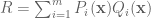 can be proved using schemes.
Here is the context: I have a bunch of cubic polynomials . I want to prove that
  is independent of
  . Also, in my problem setting I can check at as many points,
  as possible (at say W points, for some natural number W) that
 ![\hbox{rank}([\nabla f_1 \nabla f_2 ... \nabla f_{k+1}]) < (k+1)](https://s0.wp.com/latex.php?latex=%5Chbox%7Brank%7D%28%5B%5Cnabla+f_1+%5Cnabla+f_2+...+%5Cnabla+f_%7Bk%2B1%7D%5D%29+%3C+%28k%2B1%29&bg=ffffff&fg=545454&s=0&c=20201002) .
.
For that, I would like to prove: If is dependent on
  then
then ![\hbox{rank}([\nabla f_1 \nabla f_2 ... \nabla f_{k+1}]) < (k+1)](https://s0.wp.com/latex.php?latex=%5Chbox%7Brank%7D%28%5B%5Cnabla+f_1+%5Cnabla+f_2+...+%5Cnabla+f_%7Bk%2B1%7D%5D%29+%3C+%28k%2B1%29&bg=ffffff&fg=545454&s=0&c=20201002) .
.
In this proof by contradiction, suppose is dependent. Then
  vanishes wherever
  is zero (mutual zero) (Note that this is an assumption I make because of “dependence”. And the fact that experimentally at a lot of points it is true). By Hilbert’s Nullstellensatz,
  s.t.
s.t.  .
. .
.
Differentiating on both sides we get,
Evaluating it at points , I get
  , which would have nicely proved the result
 ![\hbox{rank}([\nabla f_1 \nabla f_2 ... \nabla f_{k+1}]) < (k+1)](https://s0.wp.com/latex.php?latex=%5Chbox%7Brank%7D%28%5B%5Cnabla+f_1+%5Cnabla+f_2+...+%5Cnabla+f_%7Bk%2B1%7D%5D%29+%3C+%28k%2B1%29&bg=ffffff&fg=545454&s=0&c=20201002) , except that we are not sure if
, except that we are not sure if  between 1 and k.
In which case I dont get any result as it becomes .
.
However, in case the exponent is not there, I will get
 which will give my result.
Any reference to prove / solve the above issue would be great.
Thanks in advance.
18 May, 2008 at 8:57 pm
My Conjecture « Reasonable Deviations
[…] Hilbert’s nullstellensatz Possibly related posts: (automatically generated)Existence of God […]
4 August, 2008 at 1:07 pm
Anonymous
This is late, but you might find Munshi’s proof of the Nullstellensatz interesting. It’s at http://www.math.uchicago.edu/~may/PAPERS/MunshiFinal2.pdf
It avoids harder results in commutative algebra such as Noether’s normalization theorem, and instead introduces the idea of a “flow” to prove the intersection of a maximal ideal in R[x_1, …, x_n] and R is nonempty. The proof of the weak nullstellensatz follows easily this and the strong form follows from the standard Rabinowitsch argument.
7 March, 2009 at 9:34 am
Infinite fields, finite fields, and the Ax-Grothendieck theorem « What’s new
[…] there exists a finitary algebraic obstruction that witnesses this lack of solution (see also my blog post on this topic). Specifically, suppose for contradiction that we can find a polynomial which is […]
24 April, 2009 at 6:24 pm
Hilbert Nullstellensatz « A Mind for Madness
[…] Tao proves it in a way I’ve never […]
22 June, 2009 at 9:08 pm
wuzhengpeng
Dear Prof. Tao,
I have a trivial question about the proof. How to “eliminate the role of W” in the case 1? Because RHS of (6) is linear about “W”, maybe r’ power of both sides could eliminate the role of W?
23 June, 2009 at 4:13 pm
Terence Tao
Yes, one has to raise (6) to the power r’ first; thanks for the correction!
19 July, 2009 at 4:26 pm
Why simple modules are often finite-dimensional, I « Delta Epsilons
[…] Actually proving the Nullstellensatz could make another interesting algebraic post. For now, I’ll recommend David Speyer’s interpretation of it, and Terence Tao’s elementary proof. […]
7 October, 2009 at 4:48 pm
On Hilbert’s Nullstellensatz (a non HW post) « Math840's Blog
[…] Click on the Link […]
15 October, 2009 at 7:50 pm
Reading seminar: “Stable group theory and approximate subgroups”, by Ehud Hrushovski « What’s new
[…] the -definable sets are the boolean combinations of algebraic sets; this fact is closely related to Hilbert’s nullstellensatz (and can be proven by quantifier elimination). Similarly, in the language of ordered rings, if is […]
27 November, 2009 at 4:51 pm
The weak Nullstellensatz and affine varieties « Annoying Precision
[…] weak Nullstellensatz and affine varieties November 27, 2009 Hilbert’s Nullstellensatz is a basic but foundational theorem in commutative algebra that has been discussed on the […]
26 June, 2010 at 9:28 am
The uncertainty principle « What’s new
[…] zero locus cuts out . The fundamental connection between the two perspectives is given by the nullstellensatz, which then leads to many of the basic fundamental theorems in classical algebraic […]
28 July, 2010 at 2:29 am
David Corwin
At http://mathoverflow.net/questions/33563/intuition-for-model-theoretic-proof-of-the-nullstellensatz/33576#33576, I believe I have developed an elementary and algorithmic proof of the Nullstellensatz, based largely off of a certain exposition of a model theoretic proof of it.
18 April, 2011 at 2:03 pm
J. M. Almira
Hi! Perhaps you will find interesting my paper on Nullstellensatz at Rendiconti del Circolo Matematico di Torino. The proof is elementary and, I hope, well motivated and easy to follow. You can download it from:
http://seminariomatematico.dm.unito.it/rendiconti/65-3.html
Yours,
J. M. Almira
18 May, 2011 at 1:57 pm
Lien résultant-résidu? « Exercices Aléatoires
[…] lu ici que un résultat sur le résultant du type , avec res=résultant non […]
5 July, 2011 at 2:48 pm
Polynomial bounds via nonstandard analysis « What’s new
[…] elimination theory (somewhat similar, actually, to approach I took to the nullstellensatz in my own blog post). She also notes that one could also establish the result through the machinery of Gr” obner […]
17 March, 2012 at 4:53 pm
Drei Sätze von Hilbert Ⅱ « Fight with Infinity
[…] 这种形式的零点定理在算法理论中很有用处。这里是一个基于算法精神的初等证明。 […]
16 November, 2013 at 10:12 pm
Qualitative probability theory, types, and the group chunk and group configuration theorems | What's new
[…] elimination of quantifiers in algebraically closed fields, the existence of which follows from Hilbert’s nullstellensatz) that a set is definable if and only if it is the union of a finite number of disjoint […]
22 February, 2014 at 11:07 am
Jack
For , one can explicitly give the coefficient
  in the weak nullstellensatz. Can this be done generally for
  ?
?
23 February, 2014 at 7:28 am
Jack
I’m lost in the case . It seems that when
  are not monomial, the calculation becomes rather complicated. Would you sketch your strategy for example how to find
  for
for  in
in ![{\Bbb C}[x,t]](https://s0.wp.com/latex.php?latex=%7B%5CBbb+C%7D%5Bx%2Ct%5D&bg=ffffff&fg=545454&s=0&c=20201002) ?
?
23 February, 2014 at 9:14 am
Terence Tao
The idea is to freeze all but one variable t, use the 1D theory for each choice of frozen parameters, and then glue things back together. For instance, one can set x to be (say) 57, and use the 1D theory to locate such that
  . This will be a branching process, depending on whether various expressions involving 57 vanish or not. This eventually gives a rather messy piecewise polynomial-in-57 formula for the
  in terms of a branching tree that branches depending on the vanishing or non-vanishing of various polynomials involving 57. One then has to use the algorithm described at the end of the post to collapse the tree and get genuine polynomials
  .
.
23 February, 2014 at 6:00 pm
Jack
Hmm, so the principle is to reduce the problem to which one can apply the 1D theory. I tried by Mathematica as the following :
In[35]:= f1[t_, x_] := t^2 + x^2 – 2
In[36]:= f2[t_, x_] := t*x – 1
f3[t_, x_] := t^3 + 5*t*x^2 + 1
In[38]:= g1 = Expand[-(x*t)*f1[t, x]]
Out[38]= 2 t x – t^3 x – t x^3
In[39]:= g2 = Expand[(-4*x^2 – 2)*f2[t, x]]
Out[39]= 2 – 2 t x + 4 x^2 – 4 t x^3
In[40]:= g3 = Expand[x*f3[t, x]]
Out[40]= x + t^3 x + 5 t x^3
In[41]:= g4 = g1 + g2 + g3
Out[41]= 2 + x + 4 x^2
In[42]:= g5 = Expand[x^2*f1[t, x] – (t*x + 1)*f2[t, x]]
Out[42]= 1 – 2 x^2 + x^4
In[43]:= PolynomialExtendedGCD[g4, g5, x]
Out[43]= {1, {(352 – 82 x – 142 x^2 + 47 x^3)/1225, (521 – 188 x)/
1225}}
I did it by trial and error to reduce the three polynomials in two variables to two polynomials in one variable and then use the 1D theory. I’m not sure if this is in the same spirit of your algorithm.
Using the notations in your algorithm, what we get by setting is
is  . Do we need to set other parameters, (say)
  to get
  and then go to the procedure which you call “folding up the branching tree”, or we just find
  “abstractly”?
8 July, 2014 at 12:31 pm
isomorphismes
I get that $1 \over x^2+1$ is not a polynomial, but couldn’t you represent it with an infinite series and then ${x^2 + 1 \over x^2 + 1} = 1$ identically everywhere?
8 July, 2014 at 8:53 pm
Terence Tao
Well, one can certainly work with the field of formal power series instead of the smaller ring of polynomials, but then one can no longer easily detect vanishing, which is the whole point of the Nullstellensatz. For instance, can be formally inverted by the power series
  despite the fact that it vanishes at
  .
.
9 January, 2015 at 6:15 am
Timothy P Keller ( Tim )
I have been reading Pfister’s ‘Quadratic Forms with Applications to Algebraic Geometry and Topology’. Chapter 4 has a really neat proof
of the Nullstellensatz in the homogeneous case. Unfortunately, the statement of his result ( Theorem 1.3 ) is false – but only due to a technicality –
The theorem is stated for K a p-field ( an algebraically closed field, e.g. the complex numbers, is automatically a p-field ), and R the polynomial ring over K in n + 1 variables, and f_1 , …, f_n are homogeneous polynomials ,
where for all i , p does not divide the degree of f_i.
The conclusion is that f_1, …, f_n have a common zero in K^(n+1), other than the trivial one.
For C , and R = C[X,Y], take f_1 = X, and f_2 = Y, and it’s clear the result does not hold. What’s the problem ? If one takes I = ( X,Y), then
M = R/I is isomorphic to C, i.e. dim_C ( M ) = 0. I think the result must
contain the condition that dim_C ( M ) > 0.
What do you think?
It’s a really neat ( thoroughly un-geometric, for better or worse ) proof,
and I would like to understand it thoroughly.
Thanks, Tim
8 April, 2016 at 3:03 pm
Samin Riasat
Reblogged this on Samin Riasat's Blog and commented:
Leaving it here because I want to study this at some point.
22 May, 2017 at 8:37 am
Lưu lại đề đọc sau
[…] https://terrytao.wordpress.com/2007/11/26/hilberts-nullstellensatz/ […]
6 February, 2018 at 7:27 pm
The Nullstellensatz (again) | Mark Sapir
[…] to do a blog post on the proof of Hilbert Nullstellensatz (another attempt is Terry Tao’s blog). Since I am lecturing in a few days on the Nullstellensatz, I decided to find the easiest proof, […]
9 February, 2018 at 8:48 am
Mark Sapir
Hi Terry, There is another blog post with a proof of that theorem: https://marksapir.wordpress.com/2018/02/06/the-nullstellensatz-again/
20 December, 2018 at 7:07 am
Nullstellensatz – chikurin
[…] It starts with Nullstellensatz. I am going to follow my notes, Atiyah-Macdonald, and Eisenbud. This post from Terry Tao is also a nice reading. Warning: This post would be very dry, because I don’t […]
17 April, 2020 at 11:09 am
Devendra
It’s still not concrete. I learnt this theorem when I was 19years of age. This was the occasion of the first mathematics programme in india. And i was the first indian to travel some 1800kms from my native place for the starting of this programme. It’s nothing like what a hilbert some 100yrs back and in these days the medalists have gone through during their student lives. I was quite unaware of the fact that mathematics would have taken such an industrial form. And there existed division of labour in society everywhere which has entered even mathematics. And with passage of time this led to precisely what can be called the perversion of labour. All professors started abusing me when i asked them what all those theorems simply meant in concrete forms. Only later did I come to find out that they all had gone to universities, which are nothing more than shops, at the cost of their father’s money. I was a scholarship winner but all my money was ” eaten away” by the elders in the Indian system. A knowledge of general statements generally blights the beauty which one is blessed with. Universities never serve the purpose which they profess.
3 June, 2020 at 4:07 pm
247B, Notes 4: almost everywhere convergence of Fourier series | What's new
[…] there exists a finitary algebraic obstruction that witnesses this lack of solution (see also my blog post on this topic). Specifically, suppose for contradiction that we can find a polynomial which is […]
11 April, 2021 at 7:10 pm
¿En dónde está el cero? – El paraíso de Cantor
[…] T., 2021. Hilbert’s nullstellensatz. [online] Terrence Tao’s Blog. Available at: <https://terrytao.wordpress.com/2007/11/26/hilberts-nullstellensatz/> [Accessed 8 March […]