We now begin our study of measure-preserving systems  , i.e. a probability space
  together with a probability space isomorphism
  (thus
(thus  is invertible, with T and
  both being measurable, and
  for all
  and all n). For various technical reasons it is convenient to restrict to the case when the
  -algebra
  is separable, i.e. countably generated. One reason for this is as follows:
Exercise 1. Let be a probability space with separable. Then the Banach spaces  are separable (i.e. have a countable dense subset) for every
  ; in particular, the Hilbert space
  is separable. Show that the claim can fail for
  . (We allow the
  spaces to be either real or complex valued, unless otherwise specified.)
Remark 1. In practice, the requirement that be separable is not particularly onerous. For instance, if one is studying the recurrence properties of a function  on a non-separable measure-preserving system , one can restrict to the separable sub--algebra
  generated by the level sets
  for integer n and rational q, thus passing to a separable measure-preserving system
  on which f is still measurable. Thus we see that in many cases of interest, we can immediately reduce to the separable case. (In particular, for many of the theorems in this course, the hypothesis of separability can be dropped, though we won’t bother to specify for which ones this is the case.)
We are interested in the recurrence properties of sets or functions  . The simplest such recurrence theorem is
Theorem 1. (Poincaré recurrence theorem) Let  be a measure-preserving system, and let be a set of positive measure. Then
  . In particular,
  has positive measure (and is thus non-empty) for infinitely many n.
(Compare with Theorem 1 of Lecture 3.)
Proof. For any integer  , observe that
  , and thus by Cauchy-Schwarz
 (1)
(1)
The left-hand side of (1) can be rearranged as
 (2)
(2)
On the other hand,  . From this one easily obtains the asymptotic
 (3)
(3)
where o(1) denotes an expression which goes to zero as N goes to infinity. Combining (1), (2), (3) and taking limits as  we obtain

(4)
as desired. 
Remark 2. In classical physics, the evolution of a physical system in a compact phase space is given by a (continuous-time) measure-preserving system (this is Hamilton’s equations of motion combined with Liouville’s theorem). The Poincaré recurrence theorem then has the following unintuitive consequence: every collection E of states of positive measure, no matter how small, must eventually return to overlap itself given sufficient time. For instance, if one were to burn a piece of paper in a closed system, then there exist arbitrarily small perturbations of the initial conditions such that, if one waits long enough, the piece of paper will eventually reassemble (modulo arbitrarily small error)! This seems to contradict the second law of thermodynamics, but the reason for the discrepancy is because the time required for the recurrence theorem to take effect is inversely proportional to the measure of the set E, which in physical situations is exponentially small in the number of degrees of freedom (which is already typically quite large, e.g. of the order of the Avogadro constant). This gives more than enough opportunity for Maxwell’s demon to come into play to reverse the increase of entropy. (This can be viewed as a manifestation of the curse of dimensionality.) The more sophisticated recurrence theorems we will see later have much poorer quantitative bounds still, so much so that they basically have no direct significance for any physical dynamical system with many relevant degrees of freedom.
Exercise 2. Prove the following generalisation of the Poincaré recurrence theorem: if is a measure-preserving system and  is non-negative, then
  .
.
Exercise 3. Give examples to show that the quantity  in the conclusion of Theorem 1 cannot be replaced by any larger quantity in general, regardless of the actual value of
  . (Hint: use a Bernoulli system example.)
Exercise 4. Using the pigeonhole principle instead of the Cauchy-Schwarz inequality (and in particular, the statement that if  , then the sets
  cannot all be disjoint), prove the weaker statement that for any set E of positive measure in a measure-preserving system, the set is non-empty for infinitely many n. (This exercise illustrates the general point that the Cauchy-Schwarz inequality can be viewed as a quantitative strengthening of the pigeonhole principle.)
For this lecture and the next we shall study several variants of the Poincaré recurrence theorem. We begin by looking at the mean ergodic theorem, which studies the limiting behaviour of the ergodic averages  in various spaces, and in particular in
  .
.
— Hilbert space formulation —
We begin with the Hilbert space formulation of the mean ergodic theorem, due to von Neumann.
Theorem 2. (Von Neumann ergodic theorem) Let  be a unitary operator on a separable Hilbert space H. Then for every
  we have
 , (5)
, (5)
where  is the orthogonal projection from H to the closed subspace
  consisting of the U-invariant vectors.
Proof. We give the slick (but not particularly illuminating) proof of Riesz. It is clear that (5) holds if v is already invariant (i.e.  ). Next, let W denote the (possibly non-closed) space
  . If Uw-w lies in W and v lies in
  , then by unitarity
 (6)
(6)
and thus W is orthogonal to . In particular  . From the telescoping identity
 (7)
(7)
we conclude that (5) also holds if  ; by linearity we conclude that (5) holds for all v in
  . A standard limiting argument (using the fact that the linear transformations
  and
and  are bounded on H, uniformly in n) then shows that (5) holds for v in the closure
  .
.
To conclude, it suffices to show that the closed space is all of H. Suppose for contradiction that this is not the case. Then there exists a non-zero vector w which is orthogonal to all of . In particular, w is orthogonal to Uw – w. Applying the easily verified identity  (related to the parallelogram law) we conclude that Uw=w, thus w lies in . This implies that w is orthogonal to itself and is thus zero, a contradiction.
On a measure-preserving system , the shift map  is a unitary transformation on the separable Hilbert space . We conclude
Corollary 1. (mean ergodic theorem) Let be a measure-preserving system, and let  . Then we have converges in
  norm to
  , where
  is the orthogonal projection to the space
  consists of the shift-invariant functions in
  .
.
Example 4. (Finite case) Suppose that is a finite measure-preserving system, with discrete and  the uniform probability measure. Then T is a permutation on X and thus decomposes as the direct sum of disjoint cycles (possibly including trivial cycles of length 1). Then the shift-invariant functions are precisely those functions which are constant on each of these cycles, and the map
  replaces a function
  with its average value on each of these cycles. It is then an instructive exercise to verify the mean ergodic theorem by hand in this case.
Exercise 5. With the notation and assumptions of Corollary 1, show that the limit  exists, is real, and is greater than or equal to
  . (Hint: the constant function
  lies in
  .) Note that this is stronger than the conclusion of Exercise 2.
Let us now give some other proofs of the von Neumann ergodic theorem. We first give a proof (close to von Neumann’s original proof) using the spectral theorem for unitary operators. This theorem asserts (among other things) that a unitary operator can be expressed in the form  , where
  is the unit circle and is a projection-valued Borel measure on the circle. More generally, we have
 (8)
(8)
and so for any vector v in H and any positive integer N
 . (9)
. (9)
We separate off the  portion of this integral. For
  , we have the geometric series formula
 (10)
(10)
(compare with (7)), thus we can rewrite (9) as
 . (11)
Now observe (using (10)) that  is bounded in magnitude by 1 and converges to zero as
  for any fixed . Applying the dominated convergence theorem (which requires a little bit of justification in this vector-valued case), we see that the second term in (11) goes to zero as . So we see that (9) converges to
  . But
. But  is just the orthogonal projection to the eigenspace of U with eigenvalue 1, i.e. the space , thus recovering the von Neumann ergodic theorem. (It is instructive to use spectral theory to interpret Riesz’s proof of this theorem and see how it relates to the argument just given.)
Remark 3. The above argument in fact shows that the rate of convergence in the von Neumann ergodic theorem is controlled by the spectral gap of U – i.e. how well-separated the trivial component  of the spectrum is from the rest of the spectrum. This is one of the reasons why results on spectral gaps of various operators are highly prized.
We now give another proof of Theorem 2, based on the energy decrement method; this proof is significantly lengthier, but is particularly well suited for conversion to finitary quantitative settings. For any positive integer N, define the averaging operators  ; by the triangle inequality we see that
  for all v. Now we observe
Lemma 1. (Lack of uniformity implies energy decrement) Suppose  . Then
  .
.
Proof. This follows from the identity
 (12)
(12)
and the fact that  has operator norm at most 1.
We now iterate this to obtain
Proposition 1. (Koopman-von Neumann type theorem) Let v be a unit vector, let  , and let
  be a sequence of integers with
  . Then there exists
  and a decomposition
  where
where  and
and  for all
  .
.
(The letters s, r stand for “structured” and “random” (or “residual”) respectively. For more on decompositions into structured and random components, see my FOCS lecture notes.)
Proof. We perform the following algorithm:
- Initialise j := J-1, s := 0, and r := v.
- If for all then STOP. If instead
 for some , observe from Lemma 1 that
  .
.
- Replace r with
 , replace s with
  , and replace j with j-1. Then return to Step 2.
Observe that this procedure must terminate in at most  steps (since the energy
  starts at 1, drops by at least
  at each stage, and cannot go below zero). In particular, j stays positive. Observe also that r always has norm at most 1, and thus
  at any given stage of the algorithm. From this and the triangle inequality one easily verifies the required claims.
Corollary 2 (partial von Neumann ergodic theorem). For any vector v, the averages  form a Cauchy sequence in H.
Proof. Without loss of generality we can take v to be a unit vector. Suppose for contradiction that was not Cauchy. Then one could find and  such that
  (say) for all j. By sparsifying the sequence if necessary we can assume that
  is large compared to
  ,
,  and
and  . Now we apply Proposition 1 to find
  and a decomposition v = s + r such that
  and
and  . If is large enough depending on
  , we thus have
  , and thus by the triangle inequality,
  , a contradiction.
Remark 4. This result looks weaker than Theorem 2, but the argument is much more robust; for instance, one can modify it to establish convergence of multiple averages such as  in norms for commuting shifts
  , which does not seem possible using the other arguments given here; see this paper of mine for details. Further quantitative analysis of the mean ergodic theorem can be found in this paper of Avigad, Gerhardy, and Towsner.
Corollary 2 can be used to recover Theorem 2 in its full strength, by combining it with a weak form of Theorem 2:
Proposition 2 (Weak von Neumann ergodic theorem) The conclusion (5) of Theorem 2 holds in the weak topology.
Proof. The averages lie in a bounded subset of the separable Hilbert space H, and are thus precompact in the weak topology by the sequential Banach-Alaoglu theorem. Thus, if (5) fails, then there exists a subsequence  which converges in the weak topology to some limit w other than
  . By telescoping series we see that
  , and so on taking limits we see that
  , i.e.
  . On the other hand, if y is any vector in , then
  , and thus on taking inner products with v we obtain
  . Taking limits we obtain
  , i.e. v-w is orthogonal to . These facts imply that
  , giving the desired contradiction.
— Conditional expectation —
We now turn away from the abstract Hilbert approach to the ergodic theorem (which is excellent for proving the mean ergodic theorem, but not flexible enough to handle more general ergodic theorems) and turn to a more measure-theoretic dynamics approach, based on manipulating the four components  of the underlying system separately, rather than working with the single object
  (with the unitary shift T). In particular it is useful to replace the -algebra by a sub--algebra
  , thus reducing the number of measurable functions. This creates an isometric embedding of Hilbert spaces
 (13)
(13)
and so the former space is a closed subspace of the latter. In particular, we have an orthogonal projection  , which can be viewed as the adjoint of the inclusion (13). In other words, for any ,
  is the unique element of
  such that
 (14)
(14)
for all  . (A reminder: when dealing with spaces, we identify any two functions which agree -almost everywhere. Thus, technically speaking, elements of spaces are not actually functions, but rather equivalence classes of functions.)
Example 5. (Finite case) Let X be a finite set, thus can be viewed as a partition of X, and is a coarser partition of X. To avoid degeneracies, assume that every point in X has positive measure with respect to . Then an element f of is just a function which is constant on each atom of . Similarly for  . The conditional expectation is then the function whose value on each atom A of is equal to the average value
  on that atom. (What needs to be changed here if some points have zero measure?)
We leave the following standard properties of conditional expectation as an exercise.
Exercise 6. Let be a probability space, and let be a sub--algebra. Let  .
.
- The operator
 is a bounded self-adjoint projection on . It maps real functions to real functions, it preserves constant functions (and more generally preserves
  -measurable functions), and commutes with complex conjugation.
- If f is non-negative, then
 is non-negative (up to sets of measure zero, of course). More generally, we have a comparison principle: if f, g are real-valued and
  pointwise a. e., then
  a.e. Similarly, we have the triangle inequality
  a.e..
a.e..
- (Module property) If
 , then
  a.e..
a.e..
- (Contraction) If
 for some
  , then
  . (Hint: do the p=1 and
  cases first.) This implies in particular that conditional expectation has a unique continuous extension to
  for (the case is exceptional, but note that
  is contained in since is finite).
For applications to ergodic theory, we will only be interested in taking conditional expectations with respect to a shift-invariant sub--algebra , thus  and preserve . In that case T preserves
  , and thus T commutes with conditional expectation, or in other words that
 (15)
(15)
a.e. for all 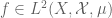 and all n.
Now we connect conditional expectation to the mean ergodic theorem. Let  be the set of essentially shift-invariant sets. One easily verifies that this is a shift-invariant sub--algebra of .
Exercise 7. Show that if E lies in  , then there exists a set
  which is genuinely invariant (TF=F) and which differs from E only by a set of measure zero. Thus it does not matter whether we deal with shift-invariance or essential shift-invariance here. (More generally, it will not make any significant difference if we modify any of the sets in our -algebras by null sets.)
The relevance of this algebra to the mean ergodic theorem arises from the following identity:
Exercise 8. Show that  .
.
As a corollary of this and Corollary 1, we have
Corollary 2. (Mean ergodic theorem, again) Let be a measure-preserving system. Then for any , the averages  converge in norm to
  .
.
Exercise 9. Show that Corollary 2 continues to hold if is replaced throughout by for any . (Hint: for the case  , use that is dense in . For the case
  , use that is dense in .) What happens when ?
Let us now give another proof of Corollary 2 (leading to a fourth proof of the mean ergodic theorem). The key here will be the decomposition  , where
  is the “structured” part of f (at least as far as the mean ergodic theorem is concerned) and
  is the “random” part. (The subscripts
  stand for “anti-uniform” and “uniform” respectively; this notation is not standard.) As
  is shift-invariant, we clearly have
 (16)
(16)
so it suffices to show that
 (17)
(17)
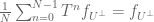
as . But we can expand out the left-hand side (using the unitarity of T) as
 (18)
(18)
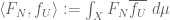
where  is the dual function of f_U, defined as
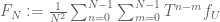 . (19)
Now, from the triangle inequality we know that the sequence of dual functions is uniformly bounded in norm, and so by Cauchy-Schwarz we know that the inner products  are bounded. If they converge to zero, we are done; otherwise, by the Bolzano-Weierstrass theorem, we have
  for some subsequence and some non-zero c.
(One could also use ultrafilters instead of subsequences here if desired, it makes little difference to the argument.) By the Banach-Alaoglu theorem (or more precisely, the sequential version of this in the separable case), there is a further subsequence  which converges weakly (or equivalently in this Hilbert space case, in the weak-* sense) to some limit
  . Since c is non-zero,
  must also be non-zero. On the other hand, from telescoping series one easily computes that
  decays like O(1/N) as , so on taking limits we have
  . In other words, lies in
  .
.
On the other hand, by construction of  we have
  . From (15) and linearity we conclude that
  for all N, so on taking limits we have
  . But since is already in , we conclude
  , a contradiction.
Remark 5. This argument is lengthier than some of the other proofs of the mean ergodic theorem, but it turns out to be fairly robust; it demonstrates (using the compactness properties of certain “dual functions”) that a function with sufficiently strong “mixing” properties (in this case, we require that  ) will cancel itself out when taking suitable ergodic averages, thus reducing the study of averages of f to the study of averages of
  . In the modern jargon, this means that is (the -algebra induced by) a characteristic factor of the ergodic average
  . We will see further examples of characteristic factors for other averages later in this course.
Exercise 10. Let  be a countably infinite discrete group. A Følner sequence is a sequence of increasing finite non-empty sets
  in
in  with
with  with the property that for any given finite set
  , we have
  as
as  , where
  is the product set of and S,
  denotes the cardinality of , and
  denotes symmetric difference. (For instance, in the case
  , the sequence
  is a Følner sequence.) If acts (on the left) in a measure-preserving manner on a probability space , and , show that
  converges in to
  , where
  is the collection of all measurable sets which are -invariant modulo null sets, and
  is the function
  .
.
[Update, Jan 30: exercise corrected, another exercise added.]
[Update, Feb 1: Some corrections.]
[Update, Feb 4: Ergodic averages changed to sum over 0 to N-1 rather than over 1 to N.]
[Update, Feb 11: Discussion of the ergodic theorem in weak topologies (Proposition 2) added.]
[Update, Feb 21: Exercise 10 corrected.]
[Update, Mar 31: Exercise 5 corrected.]
[Update, Jun 14: Some corrections.]


64 comments
Comments feed for this article
3 November, 2018 at 11:31 pm
Maths student
Unfortunately, there seems to have been a flaw in my argument, but I believe also that I see how it may be corrected.
4 November, 2018 at 12:09 am
Maths student
Apparently, the “slick” proof is the best way forward, because it seems as though no matter what, one needs to exploit the dychotomy between being in the invariant space and being orthogonal to it. Too bad that that one computation I made is not valid…
30 November, 2020 at 11:59 pm
Adam
Dear professor
I read your proof of theorem 1, and I have one question. Why inequality (3) is true?. I have tried to prove it using intuition, that the greatest element of a given set is greater than arithmetic mean of this set. I would be grateful if you gave me at least a hint.
Regards
4 December, 2020 at 12:43 pm
Terence Tao
Hint: For any one has
  such that
  for all
  except possibly for those pairs for which
  , for which one can instead use the trivial bound
  .
.
29 February, 2024 at 8:05 am
Jas, the Physicist
For exercise 1, I used that we have a sigma-finite space and not a probability space, I am wondering if I made a mistake.