We now turn to the theory of parabolic Harnack inequalities, which control the variation over space and time of solutions to the scalar heat equation
 (1)
(1)
which are bounded and non-negative, and (more pertinently to our applications) of the curvature of Ricci flows
 (2)
(2)
whose Riemann curvature  or Ricci curvature
  is bounded and non-negative. For instance, the classical parabolic Harnack inequality of Moser asserts, among other things, that one has a bound of the form
 (3)
(3)
whenever ![u: [T_-,T_+] \times M \to {\Bbb R}^+](https://s0.wp.com/latex.php?latex=u%3A+%5BT_-%2CT_%2B%5D+%5Ctimes+M+%5Cto+%7B%5CBbb+R%7D%5E%2B&bg=ffffff&fg=545454&s=0&c=20201002) is a bounded non-negative solution to (1) on a complete static Riemannian manifold M of bounded curvature,
is a bounded non-negative solution to (1) on a complete static Riemannian manifold M of bounded curvature, ![(t_1,x_1), (t_0,x_0) \in [T_-,T_+] \times M](https://s0.wp.com/latex.php?latex=%28t_1%2Cx_1%29%2C+%28t_0%2Cx_0%29+%5Cin+%5BT_-%2CT_%2B%5D+%5Ctimes+M&bg=ffffff&fg=545454&s=0&c=20201002) are spacetime points with
are spacetime points with  , and
, and  is a constant which is uniformly bounded for fixed
  when
when  range over a compact set. (The even more classical elliptic Harnack inequality gives (1) in the steady state case, i.e. for bounded non-negative harmonic functions.) In terms of heat kernels, one can view (1) as an assertion that the heat kernel associated to
  dominates (up to multiplicative constants) the heat kernel at
  .
.
The classical proofs of the parabolic Harnack inequality do not give particularly sharp bounds on the constant . Such sharp bounds were obtained by Li and Yau, especially in the case of the scalar heat equation (1) in the case of static manifolds of non-negative Ricci curvature, using Bochner-type identities and the scalar maximum principle. In fact, a stronger differential version of (3) was obtained which implied (3) by an integration along spacetime curves (closely analogous to the  -geodesics considered in earlier lectures). These bounds were particularly strong in the case of ancient solutions (in which one can send
  ). Subsequently, Hamilton applied his tensor-valued maximum principle together with some remarkably delicate tensor algebra manipulations to obtain Harnack inequalities of Li-Yau type for solutions to the Ricci flow (2) with bounded non-negative Riemannian curvature. In particular, this inequality applies to the
  -solutions introduced in the previous lecture.
In this current lecture, we shall discuss all of these inequalities (although we will not give the full details for the proof of Hamilton’s Harnack inequality, as the computations are quite involved), and derive several important consequences of that inequality for -solutions. The material here is based on several sources, including Evans’ PDE book, Müller’s book, Morgan-Tian’s book, the paper of Cao-Zhu, and of course the primary source papers mentioned in this article.
— Scalar parabolic Harnack inequalities —
Before we turn to the inequalities for Ricci flows (which are our main interest), we first consider the simpler case of scalar non-negative bounded solutions to the heat equation (1) on a static complete smooth Riemannian manifold  . This case will not actually be used in our applications but serve as an important motivating example of the method. Our basic tools will be the scalar maximum principle and the following identity.
Exercise 1. Let  be a smooth function. Establish the Bochner formula
 . (4)
. (4)
(Hint: use abstract index notation, and use the torsion-free nature of the connection, combined with the definitions of Riemann and Ricci curvature.) 
This leads to the following consequence:
Exercise 2. Let be a strictly positive solution to (1), and let  . Establish the nonlinear heat equation identities
 (5)
(5)
 (6)
(6)
 . (7)
. (7)
Now we can state the Li-Yau Harnack inequality.
Proposition 1. (Li-Yau Harnack inequality) Let M be a smooth compact d-dimensional Riemannian manifold with non-negative Ricci curvature, and let be a strictly positive smooth solution to (1). Then for every ![(t,x) \in (T_-,T_+] \times M](https://s0.wp.com/latex.php?latex=%28t%2Cx%29+%5Cin+%28T_-%2CT_%2B%5D+%5Ctimes+M&bg=ffffff&fg=545454&s=0&c=20201002) , we have
, we have
 . (8)
. (8)
Proof. By adding an epsilon to u if necessary (and then sending epsilon back to zero at the end of the argument) we may assume that  for some
  . (We shall use this trick frequently in the sequel and refer to it as the epsilon-regularisation trick.) Write and
  . From Cauchy-Schwarz we have
  , and so from (6) we see that F is a supersolution to a nonlinear heat equation:
 . (9)
. (9)
On the other hand,  is a sub-solution to the same equation, and the hypothesis that u is smooth and bounded below by
  (together with the compactness of M) implies that F dominates at times close to
  . Applying the scalar maximum principle (Corollary 1 from Lecture 3) we conclude that
  . The claim (8) now follows from (5) and the chain rule.
Remark 1. One can extend this inequality to the case when M is not compact, but is instead complete with bounded curvature, as long as one now adds the hypothesis that u is bounded (which was automatic in the compact case). The basic idea used to modify the proof is to multiply u by a suitable weight that grows at infinity to force the minimum value of F to lie in a compact set so that the maximum principle arguments can still be applied; we omit the standard details.
Remark 2. Observe that when  is Euclidean and u is the fundamental solution
  for some
  , that (8) becomes an equality.
For strictly positive ancient solutions ![u: (-\infty,0] \times M \to {\Bbb R}^+](https://s0.wp.com/latex.php?latex=u%3A+%28-%5Cinfty%2C0%5D+%5Ctimes+M+%5Cto+%7B%5CBbb+R%7D%5E%2B&bg=ffffff&fg=545454&s=0&c=20201002) to (1) on a compact manifold of non-negative Ricci curvature, one can send to negative infinity, we conclude from (8) that
to (1) on a compact manifold of non-negative Ricci curvature, one can send to negative infinity, we conclude from (8) that
 . (10)
In particular we see that  ; thus non-negative ancient solutions to the linear heat equation on compact manifolds of non-negative Ricci curvature are non-decreasing in time. [Actually, it turns out that the only such solutions are in fact constant, but we will shortly generalise this assertion to less trivial situations.]
One can linearise the inequality (10) in u, obtaining the assertion that
 (10′)
(10′)
for any vector field X. Indeed (10) and (10′) are easily seen to be equivalent by the Cauchy-Schwarz inequality. One advantage of the formulation (10′) is that it also holds true when u is merely non-negative, as opposed to strictly positive u, by the epsilon-regularisation trick. In terms of  , (10′) can also be expressed as
 (11)
(11)
although now one needs u to be strictly positive for (11) to make sense.
Now let ![(t_0,x_0), (t_1,x_1) \in (-\infty,0] \times M](https://s0.wp.com/latex.php?latex=%28t_0%2Cx_0%29%2C+%28t_1%2Cx_1%29+%5Cin+%28-%5Cinfty%2C0%5D+%5Ctimes+M&bg=ffffff&fg=545454&s=0&c=20201002) be points in spacetime with , let
be points in spacetime with , let  , and let
 ![\gamma: [0,\tau_1] \to M](https://s0.wp.com/latex.php?latex=%5Cgamma%3A+%5B0%2C%5Ctau_1%5D+%5Cto+M&bg=ffffff&fg=545454&s=0&c=20201002) be a path from
be a path from  to
to  . From the fundamental theorem of calculus and the chain rule we have
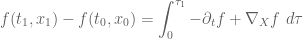 (12)
(12)
where  and the integrand is evaluated at
  . Applying (11) and then exponentiating we obtain the Harnack inequality
 (13)
(13)
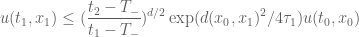
which can be extended from strictly positive solutions u to non-negative solutions u by the epsilon-regularisation trick. (Observe the similarity here with the -geodesic theory from Lecture 10.) By choosing  to be the constant-speed minimising geodesic from to , we thus conclude that
 . (14)
Remark 3. Specialising to the case when u is a static harmonic function and sending  (and using Remark 1), we recover a variant of Liouville’s theorem: a bounded harmonic function on a Riemannian manifold of bounded non-negative curvature is constant.
Exercise 3. If the non-negative solution u to (1) is not ancient, but is only restricted to a time interval ![{}[T_-,T_+]](https://s0.wp.com/latex.php?latex=%7B%7D%5BT_-%2CT_%2B%5D&bg=ffffff&fg=545454&s=0&c=20201002) , show that one still has the variant
, show that one still has the variant
 . (15)
Exercise 4. If the non-negative solution u to (1) is restricted to a time interval , and one no longer assumes that the Ricci curvature is non-negative (but it will still be bounded, since M is compact), establish the Harnack inequality (3) for some . (Hint: repeat the above arguments but with F replaced by  for some small . Show (using (6), (7)) that if is small enough, then
  obeys an inequality similar to (9) but with an additional factor of
  on the right-hand side.
Exercise 5. Establish the strong maximum principle: if M is compact and is a non-negative solution to (1) which is not identically zero, then it is strictly positive for times ![t \in (T_-,T_+]](https://s0.wp.com/latex.php?latex=t+%5Cin+%28T_-%2CT_%2B%5D&bg=ffffff&fg=545454&s=0&c=20201002) (or equivalently, if u vanishes at even one point in
(or equivalently, if u vanishes at even one point in ![(T_-,T_+] \times M](https://s0.wp.com/latex.php?latex=%28T_-%2CT_%2B%5D+%5Ctimes+M&bg=ffffff&fg=545454&s=0&c=20201002) , then it is identically zero).
, then it is identically zero).
Exercise 6. Generalise the strong maximum principle to the case when u is a supersolution  to the heat equation rather than a solution. Also generalise it to the case when the metric g is not static, but instead varies smoothly in time. (For an additional challenge, generalise further to the case when M is complete, the metric has uniformly bounded Riemann curvature, u is bounded, and one also has a drift term
  on the right-hand side of the equation for some bounded X.)
Exercise 7. Using the final generalisation of Exercise 6, as well as the evolution equation for scalar curvature (equation (31) of Lecture 1), show that the scalar curvature of a solution is strictly positive at every point in spacetime. (We will prove stronger versions of this fact later in this lecture.)
Further variants and applications of these scalar Harnack inequalities can be found in the paper of Li and Yau.
— Parabolic Harnack inequalities for the Ricci flow —
Now we turn from the scalar equation (1) to the Ricci flow equation (2), which one could think of as a kind of tensor-valued quasilinear heat equation (by de Turck’s trick, see Lecture 1). To begin with let us first consider the simple two-dimensional case d=2. In this case the Bianchi identities make the Riemann, Ricci, and scalar curvatures are all essentially equivalent (see Lecture 0); in particular one has the identity
 (16)
(16)
in the two-dimensional case. In particular, the heat equation for scalar curvature (equation (31) from Lecture 1) simplifies to
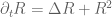 (17)
(17)
in this case; compare this with (1).
Suppose that the scalar curvature R is strictly positive. Setting  , one has an analogue of (5):
 . (18)
Exercise 8. If we set  , show the following analogue of (9):
 . (19)
[Hint: you will need to first derive the identity  for arbitrary smooth v.] Conclude that if M is compact and R is strictly positive on the time interval , then
  , and thus conclude Hamilton’s Harnack inequality for surfaces:
 . (20)
Extend this inequality to the case when R is merely non-negative rather than strictly positive by setting f equal to  rather than
  and then setting to zero (this is how should performs the epsilon regularisation trick for Ricci flow, by modifying the logarithm function by an epsilon, rather than the solution).
For ancient two-dimensional solutions with non-negative curvature, we thus conclude from the Harnack inequality (20) that R (and  ) obeys the same bounds (10), (10′), (11) that scalar solutions u did previously. In particular R is non-decreasing in time, and more generally
 (21)
(21)
for any X. We can also obtain an analogue of (13). Also, observe from the assumption of non-negative curvature and (2) that the metric is non-increasing with time, and so we can also deduce an analogue of (14):
 . (22)
With a non-trivial amount of effort, one can extend Hamilton’s Harnack inequality to higher dimensions. One cannot argue solely using the scalar curvature R, because the equation  for that curvature also involves the Ricci tensor, which thus also needs to be controlled. What is worse, one cannot argue solely using the Ricci tensor either, because the equation
 (23)
(23)
for the evolution of that curvature involves the Riemann tensor. To proceed, one in fact has to deal with the equation for the full Riemann tensor,
 (24)
(24)
where  is an explicit but rather complicated quadratic expression in the Riemann curvature. This expression simplifies when using a moving orthonormal frame, as was done in Lecture 3, to the form
 . (25)
By using (25) and many tensor calculations, one can (eventually) establish a (rather complicated) analogue of the (21) for  , and hence for and then (after taking some traces) to R. In particular, we have
Theorem 1. (Hamilton’s Harnack inequality for ancient Ricci flows) Let  be a complete ancient Ricci flow with non-negative bounded Riemann curvature. (In particular, all -solutions are of this form.) Then we have the pointwise inequality
 (26)
(26)
for any vector field X.
Note that in the two-dimensional case, (26) collapses to (23) thanks to (16).
The proof of (26) is remarkably delicate (in particular, going through the tensor curvature equation (25)), but ultimately follows broadly similar lines to the previous arguments (i.e. Bochner-type identities, Cauchy-Schwarz type inequalities, and tensor maximum principles). For technical reasons it is also convenient to carry auxiliary tensor fields such as the vector field X appearing in (26) throughout the argument. We refer the reader to Hamilton’s original paper for details. (There are alternate proofs, such as the one by Chow and Chu using a metric closely related to the high-dimensional metrics considered in Lecture 9, but all of the proofs I know of require a significant amount of calculation.)
Exercise 9. Suppose that solves the gradient steady soliton equation  for some smooth f. Using the Bianchi identity
  , establish the identity
 (27)
(27)
(note this identity also holds for gradient shrinking or expanding solitons) and then by taking divergences and using the Bianchi identity again, establish that
 . (28)
Conclude that (26) is an identity in this case when one sets  .
.
— Applications of the Harnack inequality —
Now we develop some applications of the Harnack inequality for -solutions. One easy application follows by setting X equal to 0, giving
the pointwise monotonicity of the scalar curvature in time:
 . (29)
Another application is to obtain a slightly weakened version of (22) (with the 4 in the denominator replaced by 2):
Exercise 10. Show that one has  whenever one has non-negative Riemann curvature. Using this and (26), show that
 . (30)
for all -solutions and all spacetime points  with .
Now we use the Harnack inequality to obtain some further control on the reduced length function  . Recall that this quantity takes the form
 (31)
(31)
where  and is a minimising -geodesic, which in particular means that it obeys the -geodesic equation
 (32)
(32)
(see equation (27) from Lecture 10). Using (32) and the chain rule, we can compute the total derivative  along the path
as
 . (33)
On the other hand, the Harnack inequality (26) (with X replaced by 2X) lets us bound the total derivative of R:
 . (34)
We add (33) and (34) and rearrange to obtain
![\displaystyle \frac{d}{d\tau} [\tau^{3/2} (|X|^2+R)] \leq \frac{3}{2} \sqrt{\tau} (|X|^2+R) - \tau^{1/2} |X|^2](https://s0.wp.com/latex.php?latex=%5Cdisplaystyle+%5Cfrac%7Bd%7D%7Bd%5Ctau%7D+%5B%5Ctau%5E%7B3%2F2%7D+%28%7CX%7C%5E2%2BR%29%5D+%5Cleq+%5Cfrac%7B3%7D%7B2%7D+%5Csqrt%7B%5Ctau%7D+%28%7CX%7C%5E2%2BR%29+-+%5Ctau%5E%7B1%2F2%7D+%7CX%7C%5E2&bg=ffffff&fg=545454&s=0&c=20201002) . (35)
. (35)
We (somewhat crudely) discard the non-negative  term and integrate in
  using (31) to obtain
 (36)
(36)
where we abbreviate  as l. Using the first variation formulae for reduced length (see equations (14), (15) from Lecture 11), as well as the nonnegativity of R (and hence of l), we obtain the useful inequalities
 (37)
(37)
and
 . (38)
Informally, this means that at any given point to the past of , l is roughly constant at spatial scales  and at temporal scales . Furthermore, if l is bounded, then one has bounded normalised curvature at such scales.
— A splitting theorem —
Our final application of these ideas (or more precisely, of the strong maximum principle) will be to establish a dichotomy (due to Hamilton) for 3-dimensional -solutions: either their Ricci curvature is strictly positive, or the solution splits locally as the product of a line with a two-dimensional solution.
Proposition 1. Let be a three-dimensional -solution. Suppose that the Ricci tensor has a zero eigenvalue at some point . Then on the slab  , the Ricci flow locally splits as the product of a two-dimensional Ricci flow and a line.
Proof. The first stage is to show that the Ricci tensor has a zero eigenvalue on all of
. Let  denote the three eigenvalues of the Riemann tensor as viewed in an orthonormal frame (as in Lecture 3), thus a zero eigenvalue of the Ricci tensor is equivalent to
  . Suppose for contradiction that at some time , this quantity is not identically zero, thus we can find some non-negative scalar function
  , not
, not
identically zero, such that  at time
  . We then extend h by the heat equation, so by the strong maximum principle h is strictly positive for all times after . From the convexity of the functional
  (which one can view as the minimal trace of over two-dimensional subspaces), we see that the set
  cuts out a fibrewise convex parallel subset of a suitable vector bundle over
 ![{}[t_1,t_0] \times M](https://s0.wp.com/latex.php?latex=%7B%7D%5Bt_1%2Ct_0%5D+%5Ctimes+M&bg=ffffff&fg=545454&s=0&c=20201002) (in the sense of the tensor maximum principle, Proposition 1 from Lecture 3), which one can easily check to be preserved under the ODE associated to the simultaneous evolution of (25) and the scalar heat equation for h.
(in the sense of the tensor maximum principle, Proposition 1 from Lecture 3), which one can easily check to be preserved under the ODE associated to the simultaneous evolution of (25) and the scalar heat equation for h.
Applying the tensor maximum principle we conclude that for all times in ![{}[t_1,t_0]](https://s0.wp.com/latex.php?latex=%7B%7D%5Bt_1%2Ct_0%5D&bg=ffffff&fg=545454&s=0&c=20201002) , and in particular that is non-zero at , a contradiction. Thus the Ricci curvature must have a zero eigenvalue on all of , thus
, and in particular that is non-zero at , a contradiction. Thus the Ricci curvature must have a zero eigenvalue on all of , thus  on this slab. On the other hand, from Exercise 7 we must have
  throughout this slab.
The symmetric rank 2 tensor thus has rank 1 at every point, and thus locally can be expressed in the form  for some smooth non-zero scalar a and a unit vector field v. (If M was orientable, one could extend this vector field to be global). The equation (25) then becomes

 . (39)
Since v is a unit vector field, the vector fields  are orthogonal to v for every v. Thus we can restrict to the component of (39) that is completely orthogonal to v, and conclude (since a is nonzero) that
  . If we then inspect the component of (39) which is partially orthogonal to v, we also learn that
  . Expressing the left-hand side in an orthonormal basis as the sum of rank one positive semi-definite matrices, we easily conclude that
  , i.e. v is parallel to the connection. This implies that the dual one-form
  is closed and hence locally exact; thus v is locally the gradient of some potential function f. From this we easily see that the flow locally splits as the product of a two-dimensional flow (on a level set of f) and a line (the flow lines of v), and then it is easy to verify that the two-dimensional flow is a Ricci flow, as claimed.
Remark 4. One cannot always extend this local splitting to a global one, due to topological obstructions; consider for instance the oriented round shrinking cylinder quotient (Example 3 of Lecture 12). One could also imagine the product of a round shrinking  and a static circle
  , in which the null eigenvector of the Ricci tensor splits off as a circle rather than a line; but this is not a -solution because it becomes collapsed at large scales in the distant past.
Remark 5. The above splitting analysis can be carried out in any dimension; for instance, one can show that the rank of the Riemann tensor is a constant for any ancient solution with bounded non-negative Riemann curvature. For this and further splitting results in this case, see the paper of Hamilton.


9 comments
Comments feed for this article
21 May, 2008 at 8:46 pm
285G, Lecture 14: Stationary points of Perelman entropy or reduced volume are gradient shrinking solitons « What’s new
[…] Perelman entropy, reduced volume, Ricci flow We continue our study of -solutions. In the previous lecture we primarily exploited the non-negative curvature of such solutions; in this lecture and the next, […]
27 May, 2008 at 5:58 pm
285G, Lecture 15: Geometric limits of Ricci flows, and asymptotic gradient shrinking solitons « What’s new
[…] we use the estimates on reduced length from the Harnack inequality analysis in Lecture 13 to locate some good regions of spacetime of a -solution in which to do the asymptotic analysis. […]
30 May, 2008 at 10:16 pm
285G, Lecture 16: Classification of asymptotic gradient shrinking solitons « What’s new
[…] is if the scalar curvature vanishes also. But then the strong maximum principle (Exercise 7 from Lecture 13) forces the gradient shrinking soliton to be flat at all sufficiently early times (and hence at all […]
3 June, 2008 at 12:36 pm
285G, Lecture 17: The structure of κ-solutions « What’s new
[…] curvature vanishes at any point, then by Hamilton’s splitting theorem (Proposition 1 from Lecture 13) the flow splits (locally, at least) as a line and a two-dimensional flow. Passing to a double […]
10 August, 2008 at 2:27 pm
ky
I am lost as to how you get the coefficient of 2 on (34) from (26). Please elaborate.
11 August, 2008 at 2:39 pm
Terence Tao
Dear ky,
Apply (26) with X replaced by 2X.
9 October, 2015 at 7:02 am
Azita
That was so helpful. thank you a lot.
28 December, 2020 at 6:42 pm
Adrian
Hi, Prof. Tao. Could you elaborate on Remark 1? Like what weight should we multiply exactly? Thanks.
28 December, 2020 at 10:24 pm
Terence Tao
One can find a version of this argument for instance in the original paper of Li and Yau (in Theorem 1.2; note that in the setting here one can set to zero, then send
  to infinity and
  to 1). They apply a weight in a slightly different fashion from the one suggested here but the strategy is broadly the same.