In these notes we lay out the basic theory of the Fourier transform, which is of course the most fundamental tool in harmonic analysis and also of major importance in related fields (functional analysis, complex analysis, PDE, number theory, additive combinatorics, representation theory, signal processing, etc.). The Fourier transform, in conjunction with the Fourier inversion formula, allows one to take essentially arbitrary (complex-valued) functions on a group {G} (or more generally, a space {X} that {G} acts on, e.g. a homogeneous space {G/H}), and decompose them as a (discrete or continuous) superposition of much more symmetric functions on the domain, such as characters {\chi: G \rightarrow S^1}; the precise superposition is given by Fourier coefficients {\hat f(\xi)}, which take values in some dual object such as the Pontryagin dual {\hat G} of {G}. Characters behave in a very simple manner with respect to translation (indeed, they are eigenfunctions of the translation action), and so the Fourier transform tends to simplify any mathematical problem which enjoys a translation invariance symmetry (or an approximation to such a symmetry), and is somehow “linear” (i.e. it interacts nicely with superpositions). In particular, Fourier analytic methods are particularly useful for studying operations such as convolution {f, g \mapsto f*g} and set-theoretic addition {A, B \mapsto A+B}, or the closely related problem of counting solutions to additive problems such as {x = a_1 + a_2 + a_3} or {x = a_1 - a_2}, where {a_1, a_2, a_3} are constrained to lie in specific sets {A_1, A_2, A_3}. The Fourier transform is also a particularly powerful tool for solving constant-coefficient linear ODE and PDE (because of the translation invariance), and can also approximately solve some variable-coefficient (or slightly non-linear) equations if the coefficients vary smoothly enough and the nonlinear terms are sufficiently tame.

The Fourier transform {\hat f(\xi)} also provides an important new way of looking at a function {f(x)}, as it highlights the distribution of {f} in frequency space (the domain of the frequency variable {\xi}) rather than physical space (the domain of the physical variable {x}). A given property of {f} in the physical domain may be transformed to a rather different-looking property of {\hat f} in the frequency domain. For instance:

  • Smoothness of {f} in the physical domain corresponds to decay of {\hat f} in the Fourier domain, and conversely. (More generally, fine scale properties of {f} tend to manifest themselves as coarse scale properties of {\hat f}, and conversely.)
  • Convolution in the physical domain corresponds to pointwise multiplication in the Fourier domain, and conversely.
  • Constant coefficient differential operators such as {d/dx} in the physical domain corresponds to multiplication by polynomials such as {2\pi i \xi} in the Fourier domain, and conversely.
  • More generally, translation invariant operators in the physical domain correspond to multiplication by symbols in the Fourier domain, and conversely.
  • Rescaling in the physical domain by an invertible linear transformation corresponds to an inverse (adjoint) rescaling in the Fourier domain.
  • Restriction to a subspace (or subgroup) in the physical domain corresponds to projection to the dual quotient space (or quotient group) in the Fourier domain, and conversely.
  • Frequency modulation in the physical domain corresponds to translation in the frequency domain, and conversely.

(We will make these statements more precise below.)

On the other hand, some operations in the physical domain remain essentially unchanged in the Fourier domain. Most importantly, the {L^2} norm (or energy) of a function {f} is the same as that of its Fourier transform, and more generally the inner product {\langle f, g \rangle} of two functions {f} is the same as that of their Fourier transforms. Indeed, the Fourier transform is a unitary operator on {L^2} (a fact which is variously known as the Plancherel theorem or the Parseval identity). This makes it easier to pass back and forth between the physical domain and frequency domain, so that one can combine techniques that are easy to execute in the physical domain with other techniques that are easy to execute in the frequency domain. (In fact, one can combine the physical and frequency domains together into a product domain known as phase space, and there are entire fields of mathematics (e.g. microlocal analysis, geometric quantisation, time-frequency analysis) devoted to performing analysis on these sorts of spaces directly, but this is beyond the scope of this course.)

In these notes, we briefly discuss the general theory of the Fourier transform, but will mainly focus on the two classical domains for Fourier analysis: the torus {{\Bbb T}^d := ({\bf R}/{\bf Z})^d}, and the Euclidean space {{\bf R}^d}. For these domains one has the advantage of being able to perform very explicit algebraic calculations, involving concrete functions such as plane waves {x \mapsto e^{2\pi i x \cdot \xi}} or Gaussians {x \mapsto A^{d/2} e^{-\pi A |x|^2}}.

— 1. Generalities —

Let us begin with some generalities. An abelian topological group is an abelian group {G = (G,+)} with a topological structure, such that the group operations of addition {+: G \times G \rightarrow G} and negation {-: G \rightarrow G} are continuous. (One can of course also consider abelian multiplicative groups {G = (G,\cdot)}, but to fix the notation we shall restrict attention to additive groups.) For technical reasons (and in particular, in order to apply many of the results from the previous quarter) it is convenient to restrict attention to abelian topological groups which are locally compact Hausdorff (LCH); these are known as locally compact abelian (LCA) groups.

Some basic examples of locally compact abelian groups are:

  • Finite additive groups (with the discrete topology), such as cyclic groups {{\bf Z}/N{\bf Z}}.
  • Finitely generated additive groups (with the discrete topology), such as the standard lattice {{\bf Z}^d}.
  • Tori, such as the standard {d}-dimensional torus {{\Bbb T}^d :=({\bf R}/{\bf Z})^d} with the standard topology.
  • Euclidean spaces, such the standard {d}-dimensional Euclidean space {{\bf R}^d} (with the standard topology, of course).
  • The rationals {{\bf Q}} are not locally compact with the usual topology; but if one uses the discrete topology instead, one recovers an LCA group.
  • Another example of an LCA group, of importance in number theory, is the adele ring {{\Bbb A}}, discussed in this earlier blog post.

Thus we see that locally compact abelian groups can be either discrete or continuous, and either compact or non-compact; all four combinations of these cases are of importance. The topology of course generates a Borel {\sigma}-algebra in the usual fashion, as well as a space {C_c(G)} of continuous, compactly supported complex-valued functions. There is a translation action {x \mapsto \tau_x} of {G} on {C_c(G)}, where for every {x \in G}, {\tau_x: C_c(G) \rightarrow C_c(G)} is the translation operation

\displaystyle  \tau_x f(y) := f(y-x).

LCA groups need not be {\sigma}-compact (think of the free abelian group on uncountably many generators, with the discrete topology), but one has the following useful substitute:

Exercise 1 Show that every LCA group {G} contains a {\sigma}-compact open subgroup {H}, and in particular is the disjoint union of {\sigma}-compact sets. (Hint: Take a compact symmetric neighbourhood {K} of the identity, and consider the group {H} generated by this neighbourhood.)

An important notion for us will be that of a Haar measure: a Radon measure {\mu} on {G} which is translation-invariant (i.e. {\mu(E+x) = \mu(E)} for all Borel sets {E \subset G} and all {x \in G}, where {E+x := \{ y+x: y \in E \}} is the translation of {E} by {x}). From this and the definition of integration we see that integration {f \mapsto \int_G f\ d\mu} against a Haar measure (an operation known as the Haar integral) is also translation-invariant, thus

\displaystyle  \int_G f(y-x)\ d\mu(y) = \int_G f(y)\ d\mu(y) \ \ \ \ \ (1)

or equivalently

\displaystyle  \int_G \tau_x f\ d\mu = \int_G f\ d\mu \ \ \ \ \ (2)

for all {f \in C_c(G)} and {x \in G}. The trivial measure {0} is of course a Haar measure; all other Haar measures are called non-trivial.

Let us note some non-trivial Haar measures in the four basic examples of locally compact abelian groups:

  • For a finite additive group {G}, one can take either counting measure {\#} or normalised counting measure {\#/\#(G)} as a Haar measure. (The former measure emphasises the discrete nature of {G}; the latter measure emphasises the compact nature of {G}.)
  • For finitely generated additive groups such as {{\bf Z}^d}, counting measure {\#} is a Haar measure.
  • For the standard torus {({\bf R}/{\bf Z})^d}, one can obtain a Haar measure by identifying this torus with {[0,1)^d} in the usual manner and then taking Lebesgue measure on the latter space. This Haar measure is a probability measure.
  • For the standard Euclidean space {{\bf R}^d}, Lebesgue measure is a Haar measure.

Of course, any non-negative constant multiple of a Haar measure is again a Haar measure. The converse is also true:

Exercise 2 (Uniqueness of Haar measure up to scalars) Let {\mu, \nu} be two non-trivial Haar measures on a locally compact abelian group {G}. Show that {\mu, \nu} are scalar multiples of each other, i.e. there exists a constant {c>0} such that {\nu=c\mu}. (Hint: for any {f, g \in C_c(G)}, compute the quantity {\int_G \int_G g(y) f(x+y)\ d\mu(x) d\nu(y)} in two different ways.)

The above argument also implies a useful symmetry property of Haar measures:

Exercise 3 (Haar measures are symmetric) Let {\mu} be a Haar measure on a locally compact abelian group {G}. Show that {\int_G f(-x)\ d\mu(x) = \int_G f(x)\ d\mu(x)} for all {f \in C_c(G)}. (Hint: expand {\int_G \int_G f(y) f(x+y)\ d\mu(x) d\mu(y)} in two different ways.) Conclude that Haar measures on LCA groups are symmetric in the sense that {\mu(-E) = \mu(E)} for all measurable {E}, where {-E := \{ -x: x \in E \}} is the reflection of {E}.

Exercise 4 (Open sets have positive measure) Let {\mu} be a non-trivial Haar measure on a locally compact abelian group {G}. Show that {\mu(U) > 0} for any non-empty open set {U}. Conclude that if {f \in C_c(G)} is non-negative and not identically zero, then {\int_G f\ d\mu > 0}.

Exercise 5 Let {G} be an LCA group with non-trivial Haar measure {\mu}. Let {\tilde L^\infty(G)} be the space of equivalence classes of functions {f: G \rightarrow {\bf C}} such that for every set {K} of finite measure, the restriction of {f} to {K} lies in {L^\infty(K)} with a norm bounded uniformly in {K}, with two functions in {\tilde L^\infty(G)} in the same equivalence class if they agree almost everywhere on every set {K} of finite measure, and with the {\tilde L^\infty(G)} norm of {f} equal to the supremum of the {L^\infty(K)} norms of the restrictions. (For {\sigma}-finite groups {G}, {\tilde L^\infty(G)} is identical to {L^\infty(G)}, but the two spaces differ slightly in general.) Show that {L^1(G)^*} is identifiable with {\tilde L^\infty(G)}. (Unfortunately, {G} is not always {\sigma}-finite, and so the standard duality theorem from Notes 3 of 245B does not directly apply. However, one can get around this using Exercise 1.)

It is a (not entirely trivial) theorem, due to André Weil, that all LCA groups have a non-trivial Haar measure. For discrete groups, one can of course take counting measure as a Haar measure. For compact groups, the result is due to Haar, and one can argue as follows:

Exercise 6 (Existence of Haar measure, compact case) Let {G} be a compact metrisable abelian group. For any real-valued {f \in C_c(G)}, and any Borel probability measure {\mu} on {G}, define the oscillation {\hbox{osc}_f(\mu)} of {\mu} with respect to {f} to be the quantity {\hbox{osc}_f(\mu) := \sup_{y \in G} \int_G \tau_y f\ d\mu(x) - \inf_{y \in G} \int_G \tau_y f\ d\mu(x)}.

  • (a) Show that a Borel probability measure {\mu} is a Haar measure if and only if {\hbox{osc}_f(\mu)=0} for all {f \in C_c(G)}.
  • (b) If a sequence {\mu_n} of Borel probability measures converges in the vague topology to another Borel probability measure {\mu}, show that {\hbox{osc}_f(\mu_n) \rightarrow \hbox{osc}_f(\mu)} for all {f \in C_c(G)}.
  • (c) If {\mu} is a Borel probability measure and {f \in C_c(G)} is such that {\hbox{osc}_f(\mu) > 0}, show that there exists a Borel probability measure {\mu'} such that {\hbox{osc}_f(\mu') < \hbox{osc}_f(\mu)} and {\hbox{osc}_g(\mu') \leq \hbox{osc}_g(\mu)} for all {g \in C_c(G)}. (Hint: take {\mu'} to be the an average of certain translations of {\mu}.)
  • (d) Given any finite number of functions {f_1, \ldots,f_n \in C_c(G)}, show that there exists a Borel probability measure {\mu} such that {\hbox{osc}_{f_i}(\mu)=0} for all {i=1,\ldots,n}. (Hint: Use Prokhorov’s theorem, see Corollary 13 of 245B Notes 12. Try the {n=1} case first.)
  • (e) Show that there exists a unique Haar probability measure on {G}. (Hint: One can identify each probability measure {\mu} with the element {(\int_G f\ d\mu)_{f \in C_c(G)}} of the product space {\prod_{f \in C_c(G)} [-\sup_{x \in G} |f(x)|, \sup_{x \in G} |f(x)|]}, which is compact by Tychonoff’s theorem. Now use (d) and the finite intersection property.)

(The argument can be adapted to the case when {G} is not metrisable, but one has to replace the sequential compactness given by Prokhorov’s theorem by the topological compactness given by the Banach-Alaoglu theorem.)

For general LCA groups, the proof is more complicated:

Exercise 7 (Existence of Haar measure, general case) Let {G} be an LCA group. Let {C_c(G)^+} denote the space of non-negative functions {f \in C_c(G)} that are not identically zero. Given two {f,g \in C_c(G)^+}, define a {g}-cover of {f} to be an expression of the form {a_1 \tau_{x_1} g + \ldots + a_n \tau_{x_n} g} that pointwise dominates {f}, where {a_1,\ldots,a_n} are non-negative numbers and {x_1,\ldots,x_n \in G}. Let {(f:g)} denote the infimum of the quantity {a_1+\ldots+a_n} for all {g}-covers of {f}.

  • (a) (Finiteness) Show that {0 < (f:g) < +\infty} for all {f,g \in C_c(G)^+}.
  • (b) Let {\mu} is a Haar measure on {G}. Show that {\int_G f\ d\mu \leq (f:g) (\int_G g\ d\mu)} for all {f,g \in C_c(G)^+}. Conversely, for every {f \in C_c(G)^+} and {\varepsilon > 0}, and any neighbourhood {U} of the identity, show that there exists {g \in C_c(G)^+} supported in {U} such that {\int_G f\ d\mu \geq (f:g) (\int_G g\ d\mu) - \varepsilon}. (Hint: {f} is uniformly continuous. Take {g} to be an approximation to the identity.) Thus Haar integrals are related to certain renormalised versions of the functionals {f \mapsto (f:g)}; this observation underlies the strategy for construction of Haar measure in the rest of this exercise.
  • (c) (Transitivity) Show that {(f:h) \leq (f:g) (g:h)} for all {f,g,h \in C_c(G)^+}.
  • (d) (Translation invariance) Show that {(\tau_x f:g) = (f:g)} for all {f,g \in C_c(G)^+} and {x \in G}.
  • (e) (Sublinearity) Show that {(f+g:h) \leq (f:h) + (g:h)} and {(cf:g) = c(f:g)} for all {f,g,h \in C_c(G)^+} and {c>0}.
  • (f) (Approximate superadditivity) If {f,g \in C_c(G)^+} and {\varepsilon > 0}, show that there exists a neighbourhood {U} of the identity such that {(f:h)+(g:h) \leq (1+\varepsilon) (f+g:h)} whenever {h \in C_c(G)^+} is supported in {U}. (Hint: {f, g, f+g} are all uniformly continuous. Take a {h}-cover of {f+g} and multiply the weight {a_i} at {x_i} by weights such as {f(x_i)/(f(x_i)+g(x_i)-\varepsilon)} and {g(x_i)/(f(x_i)+g(x_i)-\varepsilon)}.)

Next, fix a reference function {f_0 \in C_c(G)^+}, and define the functional {I_g: C_c(G)^+ \rightarrow {\bf R}^+} for all {g \in C_c(G)^+} by the formula {I_g(f) := (f:g) / (f_0:g)}.

  • (g) Show that for any fixed {f}, {I_g(f)} ranges in the compact interval {[(f_0:f)^{-1}, (f:f_0)]}; thus {I_g} can be viewed as an element of the product space {\prod_{f \in C_c(G)^+} [(f_0:f)^{-1}, (f:f_0)]}, which is compact by Tychonoff’s theorem.
  • (h) From (d), (e) we have the translation-invariance property {I_g(\tau_x f) = I_g(f)}, the homogeneity property {I_g(cf) = c I_g(f)}, and the sub-additivity property {I_g(f+f') \leq I_g(f)+I_g(f')} for all {g,f,f' \in C_c(G)^+}, {x \in G}, and {c>0}; we also have the normalisation {I_g(f_0)=1}. Now show that for all {f_1,\ldots,f_n,f'_1,\ldots,f'_n \in C_c(G)^+} and {\varepsilon > 0}, there exists {g \in C_c(G)^+} such that {I_g(f_i+f'_i) \geq I_g(f_i)+I_g(f'_i)-\varepsilon} for all {i=1,\ldots,n}.
  • (i) Show that there exists a unique Haar measure {\mu} on {G} with {\mu(f_0)=1}. (Hint: Use (h) and the finite intersection property to obtain a translation-invariant positive linear functional on {C_c(G)}, then use the Riesz representation theorem.)

Now we come to a fundamental notion, that of a character.

Definition 8 (Characters) Let {G} be a LCA group. A multiplicative character {\chi} is a continuous function {\chi: G \rightarrow S^1} to the unit circle {S^1 := \{ z \in {\bf C}: |z|=1\}} which is a homomorphism, i.e. {\chi(x+y)=\chi(x) \chi(y)} for all {x,y \in G}. An additive character or frequency {\xi: x \mapsto \xi \cdot x} is a continuous function {\xi: G \rightarrow {\bf R}/{\bf Z}} which is a homomorphism, thus {\xi \cdot (x+y) = \xi \cdot x + \xi \cdot y} for all {x,y \in G}. The set of all frequencies {\xi} is called the Pontryagin dual of {G} and is denoted {\hat G}; it is clearly an abelian group. A multiplicative character is called non-trivial if it is not the constant function {1}; an additive character is called non-trivial if it is not the constant function {0}.

Multiplicative characters and additive characters are clearly related: if {\xi \in \hat G} is an additive character, then the function {x \mapsto e^{2\pi i \xi \cdot x}} is a multiplicative character, and conversely every multiplicative character arises uniquely from an additive character in this fashion.

Exercise 9 Let {G} be an LCA group. We give {\hat G} the topology of local uniform convergence on compact sets, thus the topology on {\hat G} are generated by sets of the form {\{ \xi \in \hat G: |\xi \cdot x - \xi_0 \cdot x| < \varepsilon \hbox{ for all } x \in K \}} for compact {K \subset G}, {\xi_0 \in \hat G}, and {\varepsilon > 0}. Show that this turns {\hat G} into an LCA group. (Hint: Show that for any neighbourhood {U} of the identity in {G}, the sets {\{ \xi \in \hat G: \xi \cdot x \in [-\varepsilon,\varepsilon] \hbox{ for all } x \in U \}} for {0 < \varepsilon < 1/4} (say) are compact.) Furthermore, if {G} is discrete, show that {\hat G} is compact.

The Pontryagin dual can be computed easily for various classical LCA groups:

Exercise 10 Let {d \geq 1} be an integer.

  • (a) Show that the Pontryagin dual {\widehat{{\bf Z}^d}} of {{\bf Z}^d} is identifiable as an LCA group with {({\bf R}/{\bf Z})^d}, by identifying each {\xi \in ({\bf R}/{\bf Z})^d} with the frequency {x \mapsto \xi \cdot x} given by the dot product.
  • (b) Show that the Pontryagin dual {\widehat{{\bf R}^d}} of {{\bf R}^d} is identifiable as an LCA group with {{\bf R}^d}, by identifying each {\xi \in {\bf R}^d} with the frequency {x \mapsto \xi \cdot x} given by the dot product.
  • (c) Show that the Pontryagin dual {\widehat{({\bf R}/{\bf Z})^d}} of {({\bf R}/{\bf Z})^d} is identifiable as an LCA group with {{\bf Z}^d}, by identifying each {\xi \in {\bf Z}^d} with the frequency {x \mapsto \xi \cdot x} given by the dot product.
  • (d) (Contravariant functoriality) If {\phi: G \rightarrow H} is a continuous homomorphism between LCA groups, show that there is a continuous homomorphism {\phi^*: \hat H \rightarrow \hat G} between their Pontryagin duals, defined by {\phi^*(\xi) \cdot x := \xi \cdot \phi(x)} for {\xi \in \hat H} and {x \in G}.
  • (e) If {H} is a closed subgroup of an LCA group {G} (and is thus also LCA), show that {\hat H} is identifiable with {\hat G/H^\perp}, where {H^\perp} is the space of all frequencies {\xi \in \hat G} which annihilate {H} (i.e. {\xi \cdot x = 0} for all {x \in H}).
  • (f) If {G, H} are LCA groups, show that {\widehat{G \times H}} is identifiable as an LCA group with {\hat G \times \hat H}.
  • (g) Show that the Pontryagin dual of a finite abelian group {G} is identifiable with itself. (Hint: first do this for cyclic groups {{\bf Z}/N{\bf Z}}, identifying {\xi \in {\bf Z}/N{\bf Z}} with the additive character {x \mapsto x \xi/N}), then use the classification of finite abelian groups.) Note that this identification is not unique.

Exercise 11 Let {G} be an LCA group with non-trivial Haar measure {\mu}, and let {\chi: G \rightarrow S^1} be a measurable function such that {\chi(x) \chi(y) = \chi(x+y)} for almost every {x,y \in G}. Show that {\chi} is equal almost everywhere to a multiplicative character {\tilde \chi} of {G}. (Hint: on the one hand, {\tau_x \chi = \chi(-x) \chi} a.e. for almost every {x}. On the other hand, {\tau_x \chi} depends continuously on {x} in, say, the local {L^1} topology.)

In the remainder of this section, {G} is a fixed LCA group with a non-trivial Haar measure {\mu}.

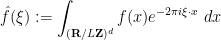
Given an absolutely integrable function {f \in L^1(G)}, we define the Fourier transform {\hat f: \hat G \rightarrow {\bf C}} by the formula

\displaystyle  \hat f(\xi) := \int_G f(x) e^{-2\pi i \xi \cdot x}\ d\mu(x).

This is clearly a linear transformation, with the obvious bound

\displaystyle  \sup_{\xi \in \hat G} |\hat f(\xi)| \leq \|f\|_{L^1(G)}.

It converts translations into frequency modulations: indeed, one easily verifies that

\displaystyle  \widehat{\tau_{x_0} f}(\xi) = e^{-2\pi i \xi \cdot x_0} \hat f(\xi) \ \ \ \ \ (3)

for any {f \in L^1(G)}, {x_0 \in G}, and {\xi \in \hat G}. Conversely, it converts frequency modulations to translations: one has

\displaystyle  \widehat{\chi_{\xi_0} f}(\xi) = \hat f(\xi-\xi_0) \ \ \ \ \ (4)

for any {f \in L^1(G)} and {\xi_0,\xi \in \hat G}, where {\chi_{\xi_0}} is the multiplicative character {\chi_{\xi_0}: x \mapsto e^{2\pi i \xi_0 \cdot x}}.

Exercise 12 (Riemann-Lebesgue lemma) If {f \in L^1(G)}, show that {\hat f: \hat G \rightarrow {\bf C}} is continuous. Furthermore, show that {\hat f} goes to zero at infinity in the sense that for every {\varepsilon > 0} there exists a compact subset {K} of {\hat G} such that {|\hat f(\xi)| \leq \varepsilon} for {\xi \not \in K}. (Hint: First show that there exists a neighbourhood {U} of the identity in {G} such that {\| \tau_x f - f \|_{L^1(G)} \leq \varepsilon^2} (say) for all {x \in U}. Now take the Fourier transform of this fact.) Thus the Fourier transform maps {L^1(G)} continuously to {C_0(\hat G)}, the space of continuous functions on {\hat G} which go to zero at infinity; the decay at infinity is known as the Riemann-Lebesgue lemma.

Exercise 13 Let {G} be an LCA group with non-trivial Haar measure {\mu}. Show that the topology of {\hat G} is the weakest topology such that {\hat f} is continuous for every {f \in L^1(G)}.

Given two {f,g \in L^1(G)}, recall that the convolution {f*g: G \rightarrow {\bf C}} is defined as

\displaystyle  f*g(x) := \int_G f(y) g(x-y)\ d\mu(y).

From Young’s inequality (Exercise 25 of Notes 1) we know that {f*g} is defined a.e., and lies in {L^1(G)}; indeed, we have

\displaystyle  \|f*g\|_{L^1(G)} \leq \|f\|_{L^1(G)} \|g\|_{L^1(G)}.

Exercise 14 Show that the operation {f, g \mapsto f*g} is a bilinear, continuous, commutative, and associative operation on {L^1(G)}. As a consequence, the Banach space {L^1(G)} with the convolution operation as “multiplication” operation becomes a commutative Banach algebra. If we also define {f^*(x) := \overline{f(-x)}} for all {f \in L^1(G)}, this turns {L^1(G)} into a Banach {*}-algebra.

For {f, g \in L^1(G)}, show that

\displaystyle  \widehat{f*g}(\xi) = \hat f(\xi) \hat g(\xi) \ \ \ \ \ (5)

for all {\xi \in \hat G}; thus the Fourier transform converts convolution to pointwise product.

Exercise 15 Let {G, H} be LCA groups with non-trivial Haar measures {\mu, \nu} respectively, and let {f \in L^1(G)}, {g \in L^1(H)}. Show that the tensor product {f \otimes g \in L^1(G \times H)} (with product Haar measure {\mu \times \nu}) has a Fourier transform of {\hat f \otimes \hat g}, where we identify {\widehat{G \times H}} with {\hat G \times \hat H} as per Exercise 10(f). Informally, this exercise asserts that the Fourier transform commutes with tensor products. (Because of this fact, the tensor power trick is often available when proving results about the Fourier transform on general groups.)

Exercise 16 (Convolution and Fourier transform of measures) If {\nu \in M(G)} is a finite Radon measure on an LCA group {G} with non-trivial Haar measure {\mu}, define the Fourier-Stieltjes transform {\hat \nu: \hat G \rightarrow {\bf C}} by the formula {\hat \nu(\xi) := \int_G e^{-2\pi i \xi \cdot x}\ d\nu(x)} (thus for instance {\hat{\mu_f} = \hat f} for any {f \in L^1(G)}). Show that {\hat \nu} is a bounded continuous function on {\hat G}. Given any {f \in L^1(G)}, define the convolution {f*\nu: G \rightarrow {\bf C}} to be the function

\displaystyle  f*\nu(x) := \int_G f(x-y)\ d\nu(y)

and given any finite Radon measure {\rho}, let {\nu*\rho: G \rightarrow {\bf C}} be the measure

\displaystyle  \nu*\rho(E) := \int_G \int_G 1_E(x+y)\ d\nu(x) d\rho(y).

Show that {f*\nu \in L^1(G)} and {\widehat{f*\nu}(\xi) = \hat f(\xi) \hat \nu(\xi)} for all {\xi \in\hat G}, and similarly that {\nu*\rho} is a finite measure and {\widehat{\nu*\rho}(\xi) = \hat \nu(\xi) \hat \rho(\xi)} for all {\xi \in \hat G}. Thus the convolution and Fourier structure on {L^1(G)} can be extended to the larger space {M(G)} of finite Radon measures.

— 2. The Fourier transform on compact abelian groups —

In this section we specialise the Fourier transform to the case when the locally compact group {G} is in fact compact, thus we now have a compact abelian group {G} with non-trivial Haar measure {\mu}. This case includes that of finite groups, together with that of the tori {({\bf R}/{\bf Z})^d}.

As {\mu} is a Radon measure, compact groups {G} have finite measure. It is then convenient to normalise the Haar measure {\mu} so that {\mu(G)=1}, thus {\mu} is now a probability measure. For the remainder of this section, we will assume that {G} is a compact abelian group and {\mu} is its (unique) Haar probability measure, as given by Exercise 6.

A key advantage of working in the compact setting is that multiplicative characters {\chi: G \rightarrow S^1} now lie in {L^2(G)} and {L^1(G)}. In particular, they can be integrated:

Lemma 17 Let {\chi} be a multiplicative character. Then {\int_G \chi\ d\mu} equals {1} when {\chi} is trivial and {0} when {\chi} is non-trivial. Equivalently, for {\xi \in \hat G}, we have {\int_G e^{2\pi i \xi \cdot x}\ d\mu = \delta_0(\xi)}, where {\delta} is the Kronecker delta function at {0}.

Proof: The claim is clear when {\chi} is trivial. When {\chi} is non-trivial, there exists {x \in G} such that {\chi(x) \neq 1}. If one then integrates the identity {\tau_x \chi = \chi(-x) \chi} using (2) one obtains the claim. \Box

Exercise 18 Show that the Pontryagin dual {\hat G} of a compact abelian group {G} is discrete (compare with Exercise 9).

Exercise 19 Show that the Fourier transform of the constant function {1} is the Kronecker delta function {\delta_0} at {0}. More generally, for any {\xi_0 \in \hat G}, show that the Fourier transform of the multiplicative character {x \mapsto e^{2\pi i \xi_0 \cdot x}} is the Kronecker delta function {\delta_{\xi_0}} at {\xi_0}.

Since the pointwise product of two multiplicative characters is again a multiplicative character, and the conjugate of a multiplicative character is also a multiplicative character, we obtain

Corollary 20 The space of multiplicative chararacters is an orthonormal set in the complex Hilbert space {L^2(G)}.

Actually, one can say more:

Theorem 21 (Plancherel theorem for compact abelian groups) Let {G} be a compact abelian group with probability Haar measure {\mu}. Then the space of multiplicative characters is an orthonormal basis for the complex Hilbert space {L^2(G)}.

The full proof of this theorem will have to wait until later notes, once we have developed the spectral theorem, though see Exercise 56 below. However, we can work out some important special cases here.

  • When {G} is a torus {G = {\Bbb T}^d = ({\bf R}/{\bf Z})^d}, the multiplicative characters {x \mapsto e^{2\pi i \xi \cdot x}} separate points (given any two {x,y \in G}, there exists a character which takes different values at {x} and at {y}). The space of finite linear combinations of multiplicative characters (i.e. the space of trigonometric polynomials) is then an algebra closed under conjugation that separates points and contains the unit {1}, and thus by the Stone-Weierstrass theorem, is dense in {C(G)} in the uniform (and hence in {L^2}) topology, and is thus dense in {L^2(G)} (in the {L^2} topology) also.
  • The same argument works when {G} is a cyclic group {{\bf Z}/N{\bf Z}}, using the multiplicative characters {x \mapsto e^{2\pi i \xi x / N}} for {\xi \in {\bf Z}/N{\bf Z}}. As every finite abelian group is isomorphic to the product of cyclic groups, we also obtain the claim for finite abelian groups.
  • Alternatively, when {G} is finite, one can argue by viewing the linear operators {\tau_x: C_c(G) \rightarrow C_c(G)} as {|G| \times |G|} unitary matrices (in fact, they are permutation matrices) for each {x \in G}. The spectral theorem for unitary matrices allows each of these matrices to be diagonalised; as {G} is abelian, the matrices commute and so one can simultaneously diagonalise these matrices. It is not hard to see that each simultaneous eigenvector of these matrices is a multiple of a character, and so the characters span {L^2(G)}, yielding the claim. (The same argument will in fact work for arbitrary compact abelian groups, once we obtain the spectral theorem for unitary operators.)

If {f \in L^2(G)}, the inner product {\langle f, \chi_\xi\rangle_{L^2(G)}} of {f} with any multiplicative character {\chi_\xi: x \mapsto e^{2\pi i \xi \cdot x}} is just the Fourier coefficient {\hat f(\xi)} of {f} at the corresponding frequency. Applying the general theory of orthonormal bases (see Notes 5), we obtain the following consequences:

Corollary 22 (Plancherel theorem for compact abelian groups, again) Let {G} be a compact abelian group with probability Haar measure {\mu}.

  • (Parseval identity) For any {f \in L^2(G)}, we have {\|f\|_{L^2(G)}^2 = \sum_{\xi \in \hat G} |\hat f(\xi)|^2}.
  • (Parseval identity, II) For any {f,g \in L^2(G)}, we have {\langle f, g \rangle_{L^2(G)} = \sum_{\xi \in \hat G} \hat f(\xi) \overline{\hat g(\xi)}}.
  • (Unitarity) Thus the Fourier transform is a unitary transformation from {L^2(G)} to {\ell^2(\hat G)}.
  • (Inversion formula) For any {f \in L^2(G)}, the series {x \mapsto \sum_{\xi \in \hat G} \hat f(\xi) e^{2\pi i \xi \cdot x}} converges unconditionally in {L^2(G)} to {f}.
  • (Inversion formula, II) For any sequence {(c_\xi)_{\xi \in \hat G}} in {\ell^2(\hat G)}, the series {x \mapsto \sum_{\xi \in \hat G} c_\xi e^{2\pi i \xi \cdot x}} converges unconditionally in {L^2(G)} to a function {f} with {c_\xi} as its Fourier coefficients.

We can record here a textbook application of the Riesz-Thorin interpolation theorem from the previous notes. Observe that the Fourier transform map {{\mathcal F}: f \mapsto \hat f} maps {L^2(G)} to {\ell^2(\hat G)} with norm {1}, and also trivially maps {L^1(G)} to {\ell^\infty(\hat G)} with norm {1}. Applying the interpolation theorem, we conclude the Hausdorff-Young inequality

\displaystyle  \| \hat f \|_{\ell^{p'}(\hat G)} \leq \|f\|_{L^p(G)} \ \ \ \ \ (6)

for all {1 \leq p \leq 2} and all {f \in L^p(G)}; in particular, the Fourier transform maps {L^p(G)} to {\ell^{p'}(\hat G)}, where {p'} is the dual exponent of {p}, thus {1/p+1/p'=1}. It is remarkably difficult (though not impossible) to establish the inequality (6) without the aid of the Riesz-Thorin theorem. (For instance, one could use the Marcinkiewicz interpolation theorem combined with the tensor power trick.) The constant {1} cannot be improved, as can be seen by testing (6) with the function {f=1} and using Exercise 19. By combining (6) with Hölder’s inequality, one concludes that

\displaystyle  \| \hat f \|_{\ell^q(\hat G)} \leq \|f\|_{L^p(G)} \ \ \ \ \ (7)

whenever {2 \leq q \leq \infty} and {\frac{1}{p}+\frac{1}{q} \leq 1}. These are the optimal hypotheses on {p,q} for which (14) holds, though we will not establish this fact here.

Exercise 23 If {f, g \in L^2(G)}, show that the Fourier transform of {fg \in L^1(G)} is given by the formula

\displaystyle  \widehat{fg}(\xi) = \sum_{\eta \in \hat G} \hat f(\eta) \hat g(\xi - \eta).

Thus multiplication is converted via the Fourier transform to convolution; compare this with (5).

Exercise 24 (Hardy-Littlewood majorant property) Let {p \geq 2} be an even integer. If {f, g \in L^p(G)} are such that {|\hat f(\xi)| \leq \hat g(\xi)} for all {\xi \in \hat G} (in particular, {\hat g} is non-negative), show that {\|f\|_{L^p(G)} \leq \|g\|_{L^p(G)}}. (Hint: use Exercise 23 and the Plancherel identity.) The claim fails for all other values of {p}, a result of Fournier.

Exercise 25 In this exercise and the next two, we will work on the torus {{\Bbb T} = {\bf R}/{\bf Z}} with the probability Haar measure {\mu}. The Pontryagin dual {\hat {\Bbb T}} is identified with {{\bf Z}} in the usual manner, thus {\hat f(n) = \int_{{\bf R}/{\bf Z}} f(x) e^{-2\pi i nx}\ dx} for all {f \in L^1({\Bbb T})}. For every integer {N > 0} and {f \in L^1({\Bbb T})}, define the partial Fourier series {S_N f} to be the expression

\displaystyle  S_N f(x) := \sum_{n=-N}^N \hat f(n) e^{2\pi i nx}.

  • Show that {S_N f = f * D_N}, where {D_N} is the Dirichlet kernel {D_N(x) := \frac{\sin(2\pi(N+1/2)x)}{\sin(\pi x)}}.
  • Show that {\|D_N\|_{L^1({\Bbb T})} \geq c \log N} for some absolute constant {c>0}. Conclude that the operator norm of {S_N} on {C({\Bbb T})} (with the uniform norm) is at least {c \log N}.
  • Conclude that there exists a continuous function {f} such that the partial Fourier series {S_N f} does not converge uniformly. (Hint: use the uniform boundedness principle.) This is despite the fact that {S_N f} must converge to {f} in {L^2} norm, by the Plancherel theorem. (Another example of non-uniform convergence of {S_N f} is given by the Gibbs phenomenon.)

Exercise 26 We continue the notational conventions of the preceding exercise. For every integer {N > 0} and {f \in L^1({\Bbb T})}, define the Césaro-summed partial Fourier series {C_N f} to be the expression

\displaystyle  C_N f(x) := \frac{1}{N} \sum_{n=0}^{N-1} D_n f(x).

  • Show that {C_N f = f * F_N}, where {F_N} is the Fejér kernel {F_N(x) := \frac{1}{n} (\frac{\sin(\pi Nx)}{\sin(\pi x)})^2}.
  • Show that {\|F_N\|_{L^1({\Bbb T})} = 1}. (Hint: what is the Fourier coefficient of {F_N} at zero?)
  • Show that {C_N f} converges uniformly to {f} for every {f \in C({\Bbb T})}. (Thus we see that Césaro averaging improves the convergence properties of Fourier series.)

Exercise 27 Carleson’s inequality asserts that for any {f \in L^2({\Bbb T})}, one has the weak-type inequality

\displaystyle  \| \sup_{N>0} |D_N f(x)| \|_{L^{2,\infty}({\Bbb T})} \leq C \|f\|_{L^2({\Bbb T})}

for some absolute constant {C}. Assuming this (deep) inequality, establish Carleson’s theorem that for any {f \in L^2({\Bbb T})}, the partial Fourier series {D_N f(x)} converge for almost every {x} to {f(x)}. (Conversely, a general principle of Stein, analogous to the uniform boundedness principle, allows one to deduce Carleson’s inequality from Carleson’s theorem. A later result of Hunt extends Carleson’s theorem to {L^p({\Bbb T})} for any {p > 1}, but a famous example of Kolmogorov shows that almost everywhere convergence can fail for {L^1({\Bbb T})} functions; in fact the series may diverge pointwise everywhere.)

— 3. The Fourier transform on Euclidean spaces —

We now turn to the Fourier transform on the Euclidean space {{\bf R}^d}, where {d \geq 1} is a fixed integer. From Exercise 10 we can identify the Pontryagin dual of {{\bf R}^d} with itself, and then the Fourier transform {\hat f: {\bf R}^d \rightarrow {\bf C}} of a function {f \in L^1({\bf R}^d)} is given by the formula

\displaystyle  \hat f(\xi) := \int_{{\bf R}^d} f(x) e^{-2\pi i \xi \cdot x}\ dx. \ \ \ \ \ (8)

Remark 28 One needs the Euclidean inner product structure on {{\bf R}^d} in order to identify {\hat{{\bf R}^d}} with {{\bf R}^d}. Without this structure, it is more natural to identify {\hat{{\bf R}^d}} with the dual space {({\bf R}^d)^*} of {{\bf R}^d}. (In the language of physics, one should interpret frequency as a covector rather than a vector.) However, we will not need to consider such subtleties here. In other areas of mathematics than harmonic analysis, the normalisation of the Fourier transform (particularly with regard to the positioning of the sign {-} and the factor {2\pi}) is sometimes slightly different from that presented here. For instance, in PDE, the factor of {2\pi} is often omitted from the exponent in order to slightly simplify the behaviour of differential operators under the Fourier transform (at the cost of introducing factors of {2\pi} in various identities, such as the Plancherel formula or inversion formula).

In Exercise 12 we saw that if {f} was in {L^1({\bf R}^d)}, then {\hat f} was continuous and decayed to zero at infinity. One can improve both the regularity and decay on {\hat f} by strengthening the hypotheses on {f}. We need two basic facts:

Exercise 29 (Decay transforms to regularity) Let {1 \leq j \leq d}, and suppose that {f, x_j f} both lie in {L^1({\bf R}^d)}, where {x_j} is the {j^{th}} coordinate function. Show that {\hat f} is continuously differentiable in the {\xi_j} variable, with

\displaystyle  \frac{\partial}{\partial \xi_j} \hat f(\xi) = -2\pi i \widehat{x_j f}(\xi).

(Hint: The main difficulty is to justify differentiation under the integral sign. Use the fact that the function {x \mapsto e^{ix}} has a derivative of magnitude {1}, and is hence Lipschitz by the fundamental theorem of calculus. Alternatively, one can show first that {\hat f(\xi)} is the indefinite integral of {-2\pi i \widehat{x_j f}} and then use the fundamental theorem of calculus.)

Exercise 30 (Regularity transforms to decay) Let {1 \leq j \leq d}, and suppose that {f \in L^1({\bf R}^d)} has a derivative {\frac{\partial f}{\partial x_j}} in {L^1({\bf R}^d)}, for which one has the fundamental theorem of calculus

\displaystyle  f(x_1,\ldots,x_n) = \int_{-\infty}^{x_j} \frac{\partial f}{\partial x_j}(x_1,\ldots,x_{j-1},t,x_{j+1},\ldots,x_n)\ dt

for almost every {x_1,\ldots,x_n}. (This is equivalent to {f} being absolutely continuous in {x_j} for almost every {x_1,\ldots,x_{j-1},x_{j+1},\ldots,x_n}.) Show that

\displaystyle  \widehat{\frac{\partial f}{\partial x_j}}(\xi) = 2\pi i \xi_j \hat f(\xi).

In particular, conclude that {|\xi_j| \hat f(\xi)} goes to zero as {|\xi| \rightarrow \infty}.

Remark 31 Exercise 30 shows that Fourier transforms diagonalise differentiation: (constant-coefficient) differential operators such as {\frac{\partial}{\partial x_j}}, when viewed in frequency space, become nothing more than multiplication operators {\hat f(\xi) \mapsto 2\pi i \xi_j \hat f(\xi)}. (Multiplication operators are the continuous analogue of diagonal matrices.) It is because of this fact that the Fourier transform is extremely useful in PDE, particularly in constant-coefficient linear PDE, or perturbations thereof.

It is now convenient to work with a class of functions which has an infinite amount of both regularity and decay.

Definition 32 (Schwartz class) A rapidly decreasing function is a measurable function {f: {\bf R}^d \rightarrow {\bf C}} such that {|x|^n f(x)} is bounded for every non-negative integer {n}. A Schwartz function is a smooth function {f: {\bf R}^d \rightarrow {\bf C}} such that all derivatives {\partial_{x_1}^{n_1} \ldots \partial_{x_d}^{n_d} f} are rapidly decreasing. The space of all Schwartz functions is denoted {{\mathcal S}({\bf R}^d)}.

Example 33 Any smooth, compactly supported function {f: {\bf R}^d \rightarrow {\bf C}} is a Schwartz function. The gaussian functions

\displaystyle  f(x) = A e^{2\pi i \theta} e^{2\pi i \xi_0 \cdot x} e^{-\pi |x - x_0|^2 / R^2} \ \ \ \ \ (9)

for {A \in {\bf R}}, {\theta \in {\bf R}/{\bf Z}}, {x_0, \xi_0 \in {\bf R}^d} are also Schwartz functions.

Exercise 34 Show that the seminorms

\displaystyle  \|f\|_{k,n} := \sup_{x \in {\bf R}^n} |x|^n |\nabla^k f(x)|

for {k,n \geq 0}, where we think of {\nabla^k f(x)} as a {d^k}-dimensional vector (or, if one wishes, a rank {k} {d}-dimensional tensor), give {{\mathcal S}({\bf R}^d)} the structure of a Fréchet space. In particular, {{\mathcal S}({\bf R}^d)} is a topological vector space.

Clearly, every Schwartz function is both smooth and rapidly decreasing. The following exercise explores the converse:

Exercise 35

  • Give an example to show that not all smooth, rapidly decreasing functions are Schwartz.
  • Show that if {f} is a smooth, rapidly decreasing function, and all derivatives of {f} are bounded, then {f} is Schwartz. (Hint: use Taylor’s theorem with remainder.)

One of the reasons why the Schwartz space is convenient to work with is that it is closed under a wide variety of operations. For instance, the derivative of a Schwartz function is again a Schwartz function, and that the product of a Schwartz function with a polynomial is again a Schwartz function. Here are some further such closure properties:

Exercise 36 Show that the product of two Schwartz functions is again a Schwartz function. Moreover, show that the product map {f, g \mapsto fg} is continuous from {{\mathcal S}({\bf R}^d) \times {\mathcal S}({\bf R}^d)} to {{\mathcal S}({\bf R}^d)}.

Exercise 37 Show that the convolution of two Schwartz functions is again a Schwartz function. Moreover, show that the convolution map {f, g \mapsto f*g} is continuous from {{\mathcal S}({\bf R}^d) \times {\mathcal S}({\bf R}^d)} to {{\mathcal S}({\bf R}^d)}.

Exercise 38 Show that the Fourier transform of a Schwartz function is again a Schwartz function. Moreover, show that the Fourier transform map {{\mathcal F}: f \mapsto \hat f} is continuous from {{\mathcal S}({\bf R}^d)} to {{\mathcal S}({\bf R}^d)}.

The other important property of the Schwartz class is that it is dense in many other spaces:

Exercise 39 Show that {{\mathcal S}({\bf R}^d)} is dense in {L^p({\bf R}^d)} for every {1 \leq p < \infty}, and is also dense in {C_0({\bf R}^d)} (with the uniform topology). (Hint: one can either use the Stone-Weierstrass theorem, or convolutions with approximations to the identity.)

Because of this density property, it becomes possible to establish various estimates and identities in spaces of rough functions (e.g. {L^p} functions) by first establishing these estimates on Schwartz functions (where it is easy to justify operations such as differentiation under the integral sign) and then taking limits.

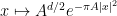
Having defined the Fourier transform {{\mathcal F}: {\mathcal S}({\bf R}^d) \rightarrow {\mathcal S}({\bf R}^d)}, we now introduce the adjoint Fourier transform {{\mathcal F}^*: {\mathcal S}({\bf R}^d) \rightarrow {\mathcal S}({\bf R}^d)} by the formula

\displaystyle  {\mathcal F}^* F(x) := \int_{{\bf R}^d} e^{2\pi i \xi \cdot x} F(\xi)\ d\xi

(note the sign change from (8)). We will shortly demonstrate that the adjoint Fourier transform is also the inverse Fourier transform: {{\mathcal F}^* = {\mathcal F}^{-1}}.

From the identity

\displaystyle  {\mathcal F}^* f = \overline{{\mathcal F} \overline{f}} \ \ \ \ \ (10)

we see that {{\mathcal F}^*} obeys much the same propeties as {{\mathcal F}}; for instance, it is also continuous from {{\mathcal S}({\bf R}^d)} to {{\mathcal S}({\bf R}^d)}. It is also the adjoint to {{\mathcal F}} in the sense that

\displaystyle  \langle {\mathcal F} f, g \rangle_{L^2({\bf R}^d)} = \langle f, {\mathcal F}^* g \rangle_{L^2({\bf R}^d)}

for all {f, g \in {\mathcal S}({\bf R}^d)}.

Now we show that {{\mathcal F}^*} inverts {{\mathcal F}}. We begin with an easy preliminary result:

Exercise 40 For any {f, g \in {\mathcal S}({\bf R}^d)}, establish the identity {{\mathcal F}^* {\mathcal F}( f * g ) = f * {\mathcal F}^* {\mathcal F} g}.

Next, we perform a computation:

Exercise 41 (Fourier transform of Gaussians) Let {r > 0}. Show that the Fourier transform of the gaussian function {g_r(x) := r^{-d} e^{-\pi |x|^2/r^2}} is {\hat g_r(\xi) = e^{-\pi r^2 |\xi|^2}}. (Hint: Reduce to the case {d=1} and {r=1}, then complete the square and use contour integration and the classical identity {\int_{-\infty}^\infty e^{-\pi x^2}\ dx = 1}.) Conclude that {{\mathcal F}^* {\mathcal F} g_r = g_r}.

Exercise 42 With {g_r} as in the previous exercise, show that {f*g_r} converges in the Schwartz space topology to {f} as {r \rightarrow 0} for all {f \in {\mathcal S}({\bf R}^d)}. (Hint: First show convergence in the uniform topology, then use the identities {\frac{\partial}{\partial x_j} (f * g ) = (\frac{\partial}{\partial x_j} f) * g} and {x_j (f*g) = (x_j f) * g + f * (x_j g)} for {f,g \in {\mathcal S}({\bf R}^d)}.)

From Exercises 40, 41 we see that

\displaystyle  {\mathcal F}^* {\mathcal F}( f*g_r ) = f*g_r

for all {r > 0} and {f \in {\mathcal S}({\bf R}^d)}. Taking limits as {r \rightarrow 0} using Exercises 38, 42 we conclude that

\displaystyle  {\mathcal F}^* {\mathcal F} f = f

for all {f \in {\mathcal S}({\bf R}^d)}, or in other words we have the Fourier inversion formula

\displaystyle  f(x) = \int_{{\bf R}^d} \hat f(\xi) e^{2\pi i \xi \cdot x}\ d\xi \ \ \ \ \ (11)

for all {x \in{\bf R}^d}. From (10) we also have

\displaystyle  {\mathcal F} {\mathcal F}^* f = f.

Taking inner products with another Schwartz function {g}, we obtain Parseval’s identity

\displaystyle  \langle {\mathcal F} f, {\mathcal F} g \rangle_{L^2({\bf R}^d)} = \langle f, g \rangle_{L^2({\bf R}^d)}

for all {f, g \in {\mathcal S}({\bf R}^d)}, and similarly for {{\mathcal F}^*}. In particular, we obtain Plancherel’s identity

\displaystyle  \| {\mathcal F} f \|_{L^2({\bf R}^d)} = \| f \|_{L^2({\bf R}^d)} = \|{\mathcal F}^* f\|_{L^2({\bf R}^d)}

for all {f \in {\mathcal S}({\bf R}^d)}. We conclude that

Theorem 43 (Plancherel’s theorem for {{\bf R}^d}) The Fourier transform operator {{\mathcal F}: {\mathcal S} \rightarrow {\mathcal S}} can be uniquely extended to a unitary transformation {{\mathcal F}: L^2({\bf R}^d) \rightarrow L^2({\bf R}^d)}.

Exercise 44 Show that the Fourier transform on {L^2({\bf R}^d)} given by Plancherel’s theorem agrees with the Fourier transform on {L^1({\bf R}^d)} given by (8) on the common domain {L^2({\bf R}^d) \cap L^1({\bf R}^d)}. Thus we may define {\hat f} for {f \in L^1({\bf R}^d)} or {f \in L^2({\bf R}^d)} (or even {f \in L^1({\bf R}^d)+L^2({\bf R}^d)} without any ambiguity (other than the usual identification of any two functions that agree almost everywhere).

Note that it is certainly possible for a function {f} to lie in {L^2({\bf R}^d)} but not in {L^1({\bf R}^d)} (e.g. the function {(1+|x|)^{-d}}). In such cases, the integrand in (8) is not absolutely integrable, and so this formula does not define the Fourier transform of {f} directly. Nevertheless, one can recover the Fourier transform via a limiting version of (8):

Exercise 45 Let {f \in L^2({\bf R}^d)}. Show that the partial Fourier integrals {\xi \mapsto \int_{|x| \leq R} f(x) e^{-2\pi i \xi \cdot x}\ dx} converge in {L^2({\bf R}^d)} to {\hat f} as {R \rightarrow \infty}.

Remark 46 It is a famous open question whether the partial Fourier integrals of an {L^2({\bf R}^d)} function also converge pointwise almost everywhere for {d \geq 2}. For {d=1}, this is essentially the celebrated theorem of Carleson mentioned in Exercise 27.

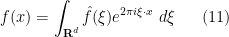
Exercise 47 (Heisenberg uncertainty principle) Let {d=1}. Define the position operator {X: {\mathcal S}({\bf R}) \rightarrow {\mathcal S}({\bf R})} and momentum operator {D: {\mathcal S}({\bf R}) \rightarrow {\mathcal S}({\bf R})} by the formulae

\displaystyle  Xf(x) := x f(x); \quad Df(x) := \frac{-1}{2\pi i} \frac{d}{dx} f(x).

Establish the identities

\displaystyle  {\mathcal F} D = X {\mathcal F}; \quad {\mathcal F} X = - {\mathcal F} D; \quad DX - XD = \frac{-1}{2\pi i} \ \ \ \ \ (12)

and the formal self-adjointness relationships

\displaystyle  \langle Xf, g \rangle_{L^2({\bf R})} = \langle f, Xg \rangle_{L^2({\bf R})}; \quad \langle Df, g \rangle_{L^2({\bf R})} = \langle f, Dg \rangle_{L^2({\bf R})}

and then establish the inequality

\displaystyle  \| Xf \|_{L^2({\bf R})} \| Df\|_{L^2({\bf R})} \geq \frac{1}{4\pi} \|f\|_{L^2({\bf R})}^2.

(Hint: start with the obvious inequality {\langle (a X + i b D) f, (aX + i bD) f \rangle_{L^2({\bf R})} \geq 0} for real numbers {a,b}, and optimise in {a} and {b}.) If {\|f\|_{L^2({\bf R})} = 1}, deduce the Heisenberg uncertainty principle

\displaystyle  [ \int_{\bf R} (\xi - \xi_0)^2 |\hat f(\xi)|^2\ d\xi]^{1/2} [ \int_{\bf R} (x - x_0)^2 |f(x)|^2\ dx]^{1/2} \geq \frac{1}{4\pi}

for any {x_0,\xi_0 \in {\bf R}}. (Hint: one can use the translation and modulation symmetries (3), (4) of the Fourier transform to reduce to the case {x_0=\xi_0=0}.) Classify precisely the {f, x_0, \xi_0} for which equality occurs.
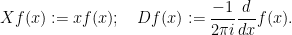
Remark 48 For {x_0,\xi_0 \in {\bf R}^d} and {R > 0}, define the gaussian wave packet {g_{x_0,\xi_0,R}} by the formula

\displaystyle  g_{x_0,\xi_0,R}(x) := 2^{d/2} R^{-d/2} e^{2\pi i \xi_0 \cdot x} e^{- \pi |x-x_0|^2 / R^2}.

These wave packets are normalised to have {L^2} norm one, and their Fourier transform is given by

\displaystyle  \hat g_{x_0,\xi_0,R} = e^{2\pi i \xi_0 \cdot x_0} g_{\xi_0,-x_0,1/R}. \ \ \ \ \ (13)

Informally, {g_{x_0,\xi_0,R}} is localised to the region {x = x_0 + O(R)} in physical space, and to the region {\xi = \xi_0 + O(1/R)} in frequency space; observe that this is consistent with the uncertainty principle. These packets “almost diagonalise” the position and momentum operators {X, D} in the sense that (taking {d=1} for simplicity)

\displaystyle  X g_{x_0,\xi_0,R} \approx x_0 g_{x_0,\xi_0,R}; \quad D g_{x_0,\xi_0,R} \approx \xi_0 g_{x_0,\xi_0,R}

(where the errors terms are morally of the form {O(R g_{x_0,\xi_0,R})} and {O( R^{-1} g_{x_0,\xi_0,R})} respectively). Of course, the non-commutativity of {D} and {X} as evidenced by the last equation in (12) shows that exact diagonalisation is impossible. Nevertheless it is useful, at an intuitive level at least, to view these wave-packets as a sort of (overdetermined) basis for {L^2({\bf R})} that approximately diagonalises {X} and {D} (as well as other formal combinations {a(X,D)} of these operators, such as differential operators or pseudodifferential operators). Meanwhile, the Fourier transform morally maps the point {(x_0,\xi_0)} in phase space to {(\xi_0,-x_0)}, as evidenced by (13) or (12); it is the model example of the more general class of Fourier integral operators, which morally move points in phase space around by canonical transformations. The study of these types of objects (which are of importance in linear PDE) is known as microlocal analysis, and is beyond the scope of this course.

The proof of the Hausdorff-Young inequality (6) carries over to the Euclidean space setting, and gives

\displaystyle  \|\hat f\|_{L^{p'}({\bf R}^d)} \leq \|f\|_{L^p({\bf R}^d)} \ \ \ \ \ (14)

for all {1 \leq p \leq 2} and all {f \in L^p({\bf R}^d)}; in particular the Fourier transform is bounded from {L^p({\bf R}^d)} to {L^{p'}({\bf R}^d)}. The constant of {1} on the right-hand side of (14) turns out to not be optimal in the Euclidean setting, in contrast to the compact setting; the sharp constant is in fact {(p^{1/p} / (p')^{1/p'})^{d/2}}, a result of Beckner. (The fact that this constant cannot be improved can be seen by using the gaussians from Exercise 41.)

Exercise 49 (Entropy uncertainty principle) For any {f \in {\mathcal S}({\bf R}^d)} with {\|f\|_{L^2({\bf R}^d)}=1}, show that

\displaystyle  - \int_{{\bf R}^d} |f(x)|^2 \log \frac{1}{|f(x)|^2}\ dx - \int_{{\bf R}^d} |\hat f(\xi)|^2 \log \frac{1}{|\hat f(\xi)|^2}\ d\xi \geq 0.

(Hint: differentiate (!) (14) in {p} at {p=2}, where one has equality in (14).) Using Beckner’s improvement to (6), improve the right-hand side to the optimal value of {d \log(2e)}.

Exercise 50 (Fourier transform under linear changes of variable) Let {L: {\bf R}^d \rightarrow {\bf R}^d} be an invertible linear transformation. If {f \in {\mathcal S}({\bf R}^d)} and {f_L(x) := f(Lx)}, show that the Fourier transform of {f_L} is given by the formula

\displaystyle  \hat f_L(\xi) = \frac{1}{|\det L|} \hat f( (L^*)^{-1} \xi )

where {L^*: {\bf R}^d \rightarrow {\bf R}^d} is the adjoint operator to {L}. Verify that this transformation is consistent with (14), and indeed shows that the exponent {p'} on the left-hand side cannot be replaced by any other exponent. (One can also establish this latter claim by dimensional analysis.)

Remark 51 As a corollary of Exercise 50, observe that if {f \in {\mathcal S}({\bf R}^d)} is spherically symmetric (thus {f = f \circ L} for all rotation matrices {L}) then {\hat f} is spherically symmetric also.

Exercise 52 (Fourier transform intertwines restriction and projection) Let {1 \leq r \leq d}, and let {f \in {\mathcal S}({\bf R}^d)}. We express {{\bf R}^d} as {{\bf R}^r \times {\bf R}^{d-r}} in the obvious manner.

  • (Restriction becomes projection) If {g \in {\mathcal S}({\bf R}^r)} is the restriction {g(x) := f(x,0)} of {f} to {{\bf R}^r \equiv {\bf R}^r \times \{0\}}, show that {\hat g(\xi) = \int_{{\bf R}^{d-r}} \hat f(\xi,\eta)\ d\eta} for all {\xi \in {\bf R}^r}.
  • (Projection becomes restriction) If {h \in {\mathcal S}({\bf R}^r)} is the projection {h(x) := \int_{{\bf R}^{d-r}} f(x,y)\ dy} of {f} to {{\bf R}^r \equiv {\bf R}^d / {\bf R}^{d-r}}, show that {\hat h(\xi) = \hat f(\xi,0)} for all {\xi \in {\bf R}^r}.

Exercise 53 (Fourier transform on large tori) Let {L > 0}, and let {({\bf R}/L{\bf Z})^d} be the torus of length {L} with Lebesgue measure {dx} (thus the total measure of this torus is {L^d}. We identify the Pontryagin dual of this torus with {\frac{1}{L} \cdot {\bf Z}^d} in the usual manner, thus we have the Fourier coefficients

\displaystyle  \hat f(\xi) := \int_{({\bf R}/L{\bf Z})^d} f(x) e^{-2\pi i \xi \cdot x}\ dx

for all {f \in L^1(({\bf R}/L{\bf Z})^d)} and {\xi \in \frac{1}{L} \cdot {\bf Z}^d}.

  • Show that for any {f \in L^2(({\bf R}/L{\bf Z})^d)}, the Fourier series {\frac{1}{L^d} \sum_{\xi \in \frac{1}{L} \cdot {\bf Z}^d} \hat f(\xi) e^{2\pi i \xi \cdot x}} converges unconditionally in {L^2(({\bf R}/L{\bf Z})^d)}.
  • Use this to give an alternate proof of the Fourier inversion formula (11) in the case where {f} is smooth and compactly supported.

Exercise 54 (Poisson summation formula) Let {f \in {\mathcal S}({\bf R}^d)}. Show that the function {F: ({\bf R}/{\bf Z})^d \rightarrow {\bf C}} defined by {F( x + {\bf Z}^d ) := \sum_{n \in{\bf Z}^d} f(x+n)} has Fourier transform {\hat F(\xi) = \hat f(\xi)} for all {\xi \in {\bf Z}^d \subset {\bf R}^d} (note the two different Fourier transforms in play here). Conclude the Poisson summation formula

\displaystyle  \sum_{n \in {\bf Z}^d} f(n) = \sum_{m \in {\bf Z}^d} \hat f(m).

Exercise 55 Let {f: {\bf R}^d \rightarrow {\bf C}} be a compactly supported, absolutely integrable function. Show that the function {\hat f} is real-analytic. Conclude that it is not possible to find a non-trivial {f \in L^1({\bf R}^d)} such that {f} and {\hat f} are both compactly supported.

— 4. The Fourier transform on general groups (optional) —

The field of abstract harmonic analysis is concerned, among other things, with extensions of the above theory to more general groups, for instance arbitrary LCA groups. One of the ways to proceed is via Gelfand theory, which for instance can be used to show that the Fourier transform is at least injective:

Exercise 56 (Fourier analysis via Gelfand theory) (Optional) In this exercise we use the Gelfand theory of commutative Banach *-algebras (see 245B Notes 12) to establish some basic facts of Fourier analysis in general groups. Let {G} be an LCA group. We view {L^1(G)} as a commutative Banach *-algebra {L^1(G)} (see Exercise 14).

  • (a) If {f \in L^1(G)} is such that {\liminf_{n \rightarrow \infty} \| f^{*n} \|_{L^1(G)}^{1/n} > 0}, where {f^{*n} = f * \ldots * f} is the convolution of {n} copies of {f}, show that there exists a non-zero complex number {z} such that the map {g \mapsto f*g - zg} is not invertible on {L^1(G)}. (Hint: If {L^1(G)} contains a unit, one can use Exercise 35 of 245B Notes 12; otherwise, adjoin a unit.)
  • (b) If {f} and {z} are as in (a), show that there exists a character {\lambda: L^1(G) \rightarrow {\bf C}} (in the sense of Banach *-algebras, see Definition 16 of 245B Notes 12) such that {f*g-zg} lies in the kernel of {\lambda} for all {g \in L^1(G)}. Conclude in particular that {\lambda(f)} is non-zero.
  • (c) If {\lambda: L^1(G) \rightarrow {\bf C}} is a character, show that there exists a multiplicative character {\chi: G \rightarrow S^1} such that {\lambda(f) = \langle f, \chi \rangle} for all {f \in L^1(G)}. (You will need Exercise 5 and Exercise 11.)
  • (d) For any {f\in L^1(G)} and {g \in L^2(G)}, show that {|f*g*g^*(0)| \leq |f*f^**g*g^*(0)|^{1/2} |g*g^*(0)|^{1/2}}, where {0} is the group identity and {f^*(x) := \overline{f(-x)}} is the conjugate of {f}. (Hint: the inner product {\langle f_1, f_2 \rangle_g := f_1 * f_2^* * g * g^*(0)} is positive semi-definite.)
  • (e) Show that if {f \in L^1(G)} is not identically zero, then there exists {\xi \in \hat G} such that {\hat f(\xi) \neq 0}. (Hint: first find {g \in L^2(G)} such that {f*g*g^*(0) \neq 0} and {g*g^*(0) \neq 0}, and conclude using (d) repeatedly that {\liminf_{n \rightarrow \infty} \| (f*f^*)^{*n} \|_{L^1(G)}^{1/n} > 0}. Then use (a), (b), (c).) Conclude that the Fourier transform is injective on {L^1(G)}. (The image of {L^1(G)} under the Fourier transform is then a Banach *-algebra known as the Wiener algebra, and is denoted {A(\hat G)}.)
  • (f) Prove Theorem 21.

It is possible to use arguments similar to those in Exercise 56 to characterise positive measures on {\hat G} in terms of continuous functions on {G}, leading to Bochner’s theorem:

Theorem 57 (Bochner’s theorem) Let {\phi \in C(G)} be a continuous function on an LCA group {G}. Then the following are equivalent:

  • (a) {\sum_{n=1}^N \sum_{m=1}^N c_n \overline{c_m} \phi( x_n - x_m ) \geq 0} for all {x_1,\ldots,x_N \in G} and {c_1,\ldots,c_N \in {\bf C}}.
  • (b) There exists a non-negative finite Radon measure {\nu} on {\hat G} such that {\phi(x) = \int_{\hat G} e^{2\pi i \xi \cdot x}\ d\nu(\xi)}.

Functions obeying either (a) or (b) are known as positive-definite functions. The space of such functions is denoted {B(G)}.

Exercise 58 Show that (b) implies (a) in Bochner’s theorem. (The converse implication is significantly harder, reprising much of the machinery in Exercise 56, but with {\phi} taking the place of {g*g^*}: see Rudin’s book for details.)

Using Bochner’s theorem, it is possible to show

Theorem 59 (Plancherel’s theorem for LCA groups) Let {G} be an LCA group with non-trivial Haar measure {\mu}. Then there exists a non-trivial Haar measure {\nu} on {\hat G} such that the Fourier transform on {L^1(G) \cap L^2(G)} can be extended continuously to a unitary transformation from {L^2(G)} to {L^2(\hat G)}. In particular we have the Plancherel identity

\displaystyle  \int_G |f(x)|^2\ d\mu(x) = \int_{\hat G} |\hat f(\xi)|^2\ d\nu(\xi)

for all {f \in L^2(G)}, and the Parseval identity

\displaystyle  \int_G f(x) \overline{g(x)}\ d\mu(x) = \int_{\hat G} \hat f(\xi) \overline{\hat g(\xi)}\ d\nu(\xi)

for all {f,g \in L^2(G)}. Furthermore, the inversion formula

\displaystyle  f(x) = \int_{\hat G} \hat f(\xi) e^{2\pi i \xi \cdot x}\ d\nu(\xi)

is valid for {f} in a dense subclass of {L^2(G)} (in particular, it is valid for {f \in L^1(G) \cap B(G)}).

Again, see Rudin’s book for details. A related result is that of Pontryagin duality: if {\hat G} is the Pontryagin dual of an LCA group {G}, then {G} is the Pontryagin dual of {\hat G}. (Certainly, every element {x \in G} defines a character {\hat x: \xi \mapsto \xi \cdot x} on {\hat G}, thus embedding {G} into {\hat{\hat G}} via the Gelfand transform; the non-trivial fact is that this embedding is in fact surjective.) One can use Pontryagin duality to convert various properties of LCA groups into other properties on LCA groups. For instance, we have already seen that {\hat G} is compact (resp. discrete) if {G} is discrete (resp. compact); with Pontryagin duality, the implications can now also be reversed. As another example, one can show that {\hat G} is connected (resp. torsion-free) if and only if {G} is torsion-free (resp. connected). We will not prove these assertions here.

It is natural to ask what happens for non-abelian locally compact groups {G = (G,\cdot)}. One can still build non-trivial Haar measures (the proof sketched out in Exercise 7 extends without difficulty to the non-abelian setting), though one must now distinguish between left-invariant and right-invariant Haar measures. (The two notions are equivalent for some classes of groups, notably compact groups, but not in general. Groups for which the two notions of Haar measures coincide are called unimodular.) However, when {G} is non-abelian then there are not enough multiplicative characters {\chi: G \rightarrow S^1} to have a satisfactory Fourier analysis. (Indeed, such characters must annihilate the commutator group {[G,G]}, and it is entirely possible for this commutator group to be all of {G}, e.g. if {G} is simple and non-abelian.) Instead, one must generalise the notion of a multiplicative character to that of a unitary representation {\rho: G \rightarrow U(H)} from {G} to the group of unitary transformations on a complex Hilbert space {H}; thus the Fourier coefficients {\hat f(\rho)} of a function will now be operators on thisl Hilbert space {H}, rather than complex numbers. When {G} is a compact group, it turns out to be possible to restrict attention to finite-dimensional representations (thus one can replace {U(H)} by the matrix group {U(n)} for some {n}). The analogue of the Pontryagin dual {\hat G} is then the collection of (irreducible) finite-dimensional unitary representations of {G}, up to isomorphism. There is an analogue of the Plancherel theorem in this setting, closely related to the Peter-Weyl theorem in representation theory. We will not discuss these topics here, but refer the reader instead to any representation theory text.

The situation for non-compact non-abelian groups (e.g. {SL_2({\bf R})}) is significantly more subtle, as one must now consider infinite-dimensional representations as well as finite-dimensional ones, and the inversion formula can become quite non-trivial (one has to decide what “weight” each representation should be assigned in that formula). At this point it seems unprofitable to work in the category of locally compact groups, and specialise to a more structured class of groups, e.g. algebraic groups. The representation theory of such groups is a massive subject and well beyond the scope of this course.

— 5. Relatives of the Fourier transform (optional) —

There are a number of other Fourier-like transforms used in mathematics, which we will briefly survey here. Firstly, there are some rather trivial modifications one can make to the definition of Fourier transform, for instance by replacing the complex exponential {e^{2\pi i x}} by trigonometric functions such as {\sin(x)} and {\cos(x)}, or moving around the various factors of {2\pi}, {i}, {-1}, etc. in the definition. In this spirit, we have the Laplace transform

\displaystyle  {\mathcal L} f(t) :=\int_0^\infty f(s) e^{-st}\ ds \ \ \ \ \ (15)

of a measurable function {f: [0,+\infty) \rightarrow {\bf R}} with some reasonable growth at infinity, where {t > 0}. Roughly speaking, the Laplace transform is “the Fourier transform without the {i}” (cf. Wick rotation), and so has the (mild) advantage of being definable in the realm of real-valued functions rather than complex-valued functions. It is particularly well suited for studying ODE on the half-line {[0,+\infty)} (e.g. initial value problems for a finite-dimensional system). The Laplace transform and Fourier transform can be unified by allowing the {t} parameter in (15) to vary in the right-half plane {\{ t \in {\bf C}: \hbox{Re}(t) \geq 0 \}}.

When the Fourier transform is applied to a spherically symmetric function {f(x) := F(|x|)} on {{\bf R}^d}, then the Fourier transform is also spherically symmetric, given by the formula {\hat f(\xi) = G(|\xi|)} where {G} is the Fourier-Bessel transform (or Hankel transform)

\displaystyle  G(r) := 2\pi r^{-(d-2)/2} \int_0^\infty F(s) J_{(d-2)/2}(2\pi r s) s^{d/2}\ ds

where {J_\nu} is the Bessel function of the first kind with index {\nu}. In practice, one can then analyse the Fourier-analytic behaviour of spherically symmetric functions in terms of one-dimensional Fourier-like integrals by using various asymptotic expansions of the Bessel function.

There is a relationship between the {d}-dimensional Fourier transform and the one-dimensional Fourier transform, provided by the Radon transform, defined for {f \in {\mathcal S}({\bf R}^d)} (say) by the formula

\displaystyle  {\mathcal R}f( \omega, t ) := \int_{x \cdot \omega = t} f

where {\omega \in S^{d-1}}, {t \in {\bf R}}, and the integration is with respect to {d-1}-dimensional measure. Indeed one checks that the {d}-dimensional Fourier transform of {f} at {r \omega} for some {r > 0} and {\omega \in S^{d-1}} is nothing more than the one-dimensional Fourier coefficient of the function {t \mapsto {\mathcal R} f(\omega,t)} at {r}. The Radon transform is often used in scattering theory and related areas of analysis, geometry, and physics.

In analytic number theory, a multiplicative version of the Fourier-Laplace transform is often used, namely the Mellin transform

\displaystyle  {\mathcal M} f(s) := \int_0^\infty x^s f(x)\frac{dx}{x}.

(Note that {\frac{dx}{x}} is a Haar measure for the multiplicative group {{\bf R}^+ = (0,+\infty)}.) To see the relation with the Fourier-Laplace transform, write {f(x) = F(\log x)}, then the Mellin transform becomes

\displaystyle  {\mathcal M} f(s) = \int_{\bf R} e^{st} f(t)\ dt.

Many functions of importance in analytic number theory, such as the Gamma function or the zeta function, can be expressed neatly in terms of Mellin transforms.

In electrical engineering and signal processing, the z-transform is often used, transforming a sequence {c = (c_n)_{n=-\infty}^\infty} of complex numbers to a formal Laurent series

\displaystyle  {\mathcal Z} c(z) := \sum_{n=-\infty}^\infty c_n z^n

(some authors use {z^{-n}} instead of {z^n} here). If one makes the substitution {z = e^{2\pi i nx}} then this becomes a (formal) Fourier series expansion on the unit circle. If the sequence {c_n} is restricted to only be non-zero for non-negative {n}, and does not grow too quickly as {n \rightarrow \infty}, then the {z}-transform becomes holomorphic on the unit disk, thus providing a link between Fourier analysis and complex analysis. For instance, the standard formula

\displaystyle  c_n = \frac{1}{2\pi i} \int_{|z|=1} \frac{f(z)}{z^{n+1}}\ dz

for the Taylor coefficients of a holomorphic function {f(z) = \sum_{n=0}^\infty c_n z^n} at the origin can be viewed as a version of the Fourier inversion formula for the torus {{\bf R}/{\bf Z}}. Just as the Fourier or Laplace transforms are useful for analysing differential equations in continuous settings, the {z}-transform is useful for analysing difference equations in discrete settings. The {z}-transform is of course also very similar to the method of generating functions in combinatorics and probability.

In probability theory one also considers the characteristic function {{\Bbb E}(e^{itX})} of a real-valued random variable {X}; this is essentially the Fourier transform of the probability distribution of {X}. Just as the Fourier transform is useful for understanding convolutions {f*g}, the characteristic function is useful for understanding sums {X_1+X_2} of independent random variables.

We have briefly touched upon the role of Gelfand theory in the general theory of the Fourier transform. Indeed, one can view the Fourier transform as the special case of the Gelfand transform for Banach *-algebras, which we already discussed in 245B Notes 12.

The Fast Fourier Transform (FFT) is not, strictly speaking, a variant of the Fourier transform, but rather is an efficient algorithm for computing the Fourier transform

\displaystyle  \hat f(\xi) = \frac{1}{N} \sum_{n=0}^{N-1} f(x) e^{-2\pi i \xi x/N}

on a cyclic group {{\bf Z}/N{\bf Z} \equiv \{0,\ldots,N-1\}}, when {N} is large but composite. Note that a brute force computation of this transform for all {N} values of {\xi} would require about {O(N^2)} addition and multiplication operations. The FFT algorithm, in contrast, takes only {O(N \log N)} operations, and is based on reducing the FFT for a large {N} to FFT for smaller {N}. For instance, suppose {N} is even, say {N=2M}, then observe that

\displaystyle  \hat f(\xi) = \frac{1}{2} ( \hat f_0(\xi) + e^{-2\pi i \xi / N } \hat f_1(\xi) )

where {f_0, f_1: {\bf Z}/M{\bf Z} \rightarrow {\bf C}} are the functions {f_j(x) := f(2x+j)}. Thus one can obtain the Fourier transform of the length {N} vector {f} from the Fourier transforms of the two length {M} vectors {f_0, f_1} after about {O(N)} operations. Iterating this we see that we can indeed compute {\hat f} in {O( N \log N )} operations, at least in the model case when {N} is a power of two; the general case has a similar but more complicated analysis.

In many situations (particularly in ergodic theory), it is desirable not to perform Fourier analysis on a group {G} directly, but instead on another space {X} that {G} acts on. Suppose for instance that {G} is a compact abelian group, with probability Haar measure {dg}, which acts in a measure-preserving (and measurable) fashion on a probability space {(X,\mu)}. Then one can decompose any {f \in L^2(X)} into Fourier components {f = \sum_{\xi \in \hat G} f_\xi}, where {f_\xi(x) := \int_G e^{-2\pi i \xi \cdot g} f(g x)\ dg}, where the series is unconditionally convergent in {L^2(X)}. The reason for doing this is that each of the {f_\xi} behaves in a simple way with respect to the group action, indeed one has {f_\xi( g x ) = e^{2\pi i \xi \cdot g} f_\xi(x)} for (almost) all {g \in G, x \in X}. This decomposition is closely related to the decomposition in representation theory of a given representation into irreducible components. Perhaps the most basic example of this type of operation is the decomposition of a function {f: {\bf R} \rightarrow {\bf R}} into even and odd components {\frac{f(x)+f(-x)}{2}}, {\frac{f(x)-f(-x)}{2}}; here the underlying group is {{\bf Z}/2{\bf Z}}, which acts on {{\bf R}} by reflections, {gx := (-1)^g x}.

The operation of converting a square matrix {A = (a_{ij})_{1 \leq i,j \leq n}} of numbers into eigenvalues {\lambda_1,\ldots,\lambda_n} or singular values {\sigma_1,\ldots,\sigma_n} can be viewed as a sort of non-commutative generalisation of the Fourier transform. (Note that the eigenvalues of a circulant matrix are essentially the Fourier coefficients of the first row of that matrix.) For instance, the identity {\sum_{i=1}^n \sum_{j=1}^n |a_{ij}|^2 = \sum_{k=1}^n \sigma_k^2} can be viewed as a variant of the Plancherel identity. More generally, there are close relationships between spectral theory and Fourier analysis (as one can already see from the connection to Gelfand theory). For instance, in {{\bf R}^d} and {{\Bbb T}^d}, one can view Fourier analysis as the spectral theory of the gradient operator {\nabla} (note that the characters {e^{2\pi i \xi \cdot x}} are joint eigenfunctions of {\nabla}). As the gradient operator is closely related to the Laplacian {\Delta}, it is not surprising that Fourier analysis is also closely related to the spectral theory of the Laplacian, and in particular to various operators built using the Laplacian (e.g. resolvents, heat kernels, wave operators, Schrödinger operators, Littlewood-Paley projections, etc.). Indeed, the spectral theory of the Laplacian can serve as a partial substitute for the Fourier transform in situations in which there is not enough symmetry to exploit Fourier-analytic techniques (e.g. on a manifold with no translation symmetries).

Finally, there is an analogue of the Fourier duality relationship between an LCA group {G} and its Pontryagin dual {\hat G} in algebraic geometry, known as the Fourier-Mukai transform, which relates an abelian variety {X} to its dual {\hat X}, and transforms coherent sheaves on the former to coherent sheaves on the latter. This transform obeys many of the algebraic identities that the Fourier transform does, although it does not seem to have much of the analytic structure.