
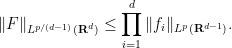
As discussed in previous notes, a function space norm can be viewed as a means to rigorously quantify various statistics of a function 


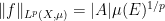


However, there are more features of a function 

- Let
be a test function that equals
near the origin, and
be a large number. Then the function
oscillates at a wavelength of about
, and a frequency scale of about
; for instance, the derivative
grows at a roughly linear rate as
- Continuing the previous example, now consider the function
, where
is some parameter. This function also has a frequency scale of about
derivative of
stays bounded in
. So one could view this function as having “
degrees of regularity” in the limit
- In a similar vein, the function
also has a frequency scale of about
- The function
also has about
variable, one can also decompose this function into components
for
, where
is a bump function supported away from the origin; each such component has frequency scale about
and
.
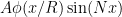
- One can of course concoct higher-dimensional analogues of these examples. For instance, the localised plane wave
in
is a test function, would have a frequency scale of about
.
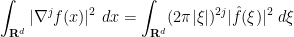
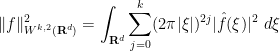
There are a variety of function space norms that can be used to capture frequency scale (or regularity) in addition to height and width. The most common and well-known examples of such spaces are the Sobolev space norms 


To a large extent, the theory of the Sobolev spaces 


The uncertainty principle in Fourier analysis places a constraint between the width and frequency scale of a function; roughly speaking (and in one dimension for simplicity), the product of the two quantities has to be bounded away from zero (or to put it another way, a wave is always at least as wide as its wavelength). This constraint can be quantified as the very useful Sobolev embedding theorem, which allows one to trade regularity for integrability: a function in a Sobolev space 


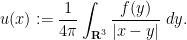
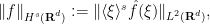
Plancherel’s theorem reveals that Fourier-analytic tools are particularly powerful when applied to 


We will not fully develop the theory of Sobolev spaces here, as this would require the theory of singular integrals, which is beyond the scope of this course. There are of course many references for further reading; one is Stein’s “Singular integrals and differentiability properties of functions“.
— 1. Hölder spaces —
Throughout these notes, 
Before we study Sobolev spaces, let us first look at the more elementary theory of Hölder spaces 

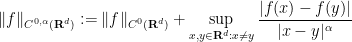
We first recall the 


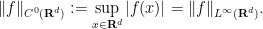
This norm gives 

where we view 


(One does not have to use the 

Remark 1 In some texts,
would lie in
for every
(i.e. they are locally in
(smooth functions, with no bounds on derivatives) and
(smooth functions, all of whose derivatives are bounded). Thus, for instance,
but not
.
Exercise 2 Show that
Exercise 3 Show that for every
, the
in the sense that there exists a constant
(depending on
for all
. (Hint: use Taylor series with remainder.) Thus when defining the
; the two extreme terms
suffice. (This is part of a more general interpolation phenomenon; the extreme terms in a sum often already suffice to control the intermediate terms.)


Exercise 4 Let
with
,
, and
, then the function
has a
, where
, and frequency scale
We clearly have the inclusions

and for any constant-coefficient partial differential operator
of some order 


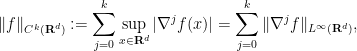
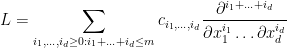
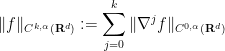
The Hölder spaces 


is finite. To put it another way, 

for some constant 

The space 


Exercise 5 Show that
is a Banach space for every
Exercise 6 Show that
for every
, and that the inclusion map is continuous.
Exercise 7 If
, show that the
to be less than or equal to
Exercise 8 Show that
is a proper subspace of
norm. (The relationship between
, as can be seen from the fundamental theorem of calculus.)
Exercise 9 Let
be a distribution. Show that
if and only if
. Furthermore, for
is comparable to
.
We can then define the
is finite. (As before, there are a variety of ways to define the
Exercise 10 Show that
, and is contained in turn in
As before, 


Exercise 11 Let
.
- Show that the function
lies in
whenever
.
- Conversely, if
, and
, show that
- Show that
lies in
, but not in
.
This example illustrates that the quantity
can be viewed as measuring the total amount of regularity held by functions in
Exercise 12 Let
, for some
.
By construction, it is clear that continuously differential operators 

Now we consider what happens with products.
Exercise 13 Let
be natural numbers, and
.
- If
, show that
, and that the multiplication map is continuous from
to
. (Hint: reduce to the case
and use induction.)
- If
and
, and
, show that
, and that the multiplication map is continuous from
to
It is easy to see that the regularity in these results cannot be improved (just take
). This illustrates a general principle, namely that a pointwise product
tends to acquire the lower of the regularities of the two factors
.
As one consequence of this exercise, we see that any variable-coefficient differential operator 
We now briefly remark on Hölder spaces on open domains 


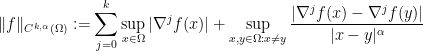
is finite; this is the “maximal” choice for the 


Exercise 14 Let
. Show that
is a dense subset of
if one places the
topology on the latter space. (Hint: To approximate a compactly supported
one, convolve with a smooth, compactly supported approximation to the identity.) What happens in the endpoint case
?
Hölder spaces are particularly useful in elliptic PDE, because tools such as the maximum principle lend themselves well to the suprema that appear inside the definition of the 
Exercise 15 (Schauder estimate) Let
be a function supported on the unit ball
. Let
be the unique bounded solution to the Poisson equation
is the Laplacian), given by convolution with the Newton kernel:
- (i) Show that
.
- (ii) Show that
, and rigorously establish the formula
for
.
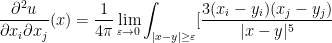
- (iii) Show that
, and rigorously establish the formula
for
, where
is the Kronecker delta. (Hint: first establish this in the two model cases when
, and when
- (iv) Show that
, and establish the Schauder estimate
where
depends only on
- (v) Show that the Schauder estimate fails when
. Using this, conclude that there eixsts
supported in the unit ball such that the function
. (Hint: use the closed graph theorem.) This failure helps explain why it is necessary to introduce Hölder spaces into elliptic theory in the first place (as opposed to the more intuitive

![\displaystyle - \frac{\delta_{ij}}{|x-y|^3}] f(y)\ dy](https://s0.wp.com/latex.php?latex=%5Cdisplaystyle+-+%5Cfrac%7B%5Cdelta_%7Bij%7D%7D%7B%7Cx-y%7C%5E3%7D%5D+f%28y%29%5C+dy&bg=ffffff&fg=000000&s=0&c=20201002)

Remark 16 Roughly speaking, the Schauder estimate asserts that if
has
being an elliptic differential operator. We will discus ellipticity a little bit more later in Exercise 45. The theory of Schauder estimates is by now extremely well developed, and applies to large classes of elliptic operators on quite general domains, but we will not discuss these estimates and their applications to various linear and nonlinear elliptic PDE here.
Exercise 17 (Rellich-Kondrachov type embedding theorem for Hölder spaces) Let
. Show that any bounded sequence of functions
that are all supported in the same compact subset of
will have a subsequence that converges in
— 2. Classical Sobolev spaces —
We now turn to the “classical” Sobolev spaces 
Definition 18 Let
, and let
. If
norm of
(As before, the exact choice of convention in which one measures the
is not particularly relevant for most applications, as all such conventions are equivalent up to multiplicative constants.)

The space 
Example 19
is of course the same space as
is the same space as
, with an equivalent norm. More generally, one can see from induction that
is the same space as
for any
.
Example 20 The function
lies in
. On the other hand, the Cantor function (aka the “Devil’s staircase”) is not in
Exercise 21 Let
norm of at most
, where
and
Exercise 22 Show that
The fact that Sobolev spaces are defined using weak derivatives is a technical nuisance, but in practice one can often end up working with classical derivatives anyway by means of the following lemma:
Lemma 23 Let
and
Proof: It is clear that 
We begin with the former claim. Let 


Now we prove the latter claim. Let 


As a corollary of this lemma we also see that the space 
Exercise 24 Let
is
(the space of
functions whose first
.
Now we come to the important Sobolev embedding theorem, which allows one to trade regularity for integrability. We illustrate this phenomenon first with some very simple cases. First, we claim that the space 


for all test functions 

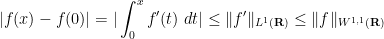
for all

Also, taking

and (1) follows.
Since the closure of 

Exercise 25 Show that
embeds continuously into
, thus there exists a constant
for all
.

Now we turn to Sobolev embedding for exponents other than 
Theorem 26 (Sobolev embedding theorem for one derivative) Let
be such that
, but that one is not in the endpoint cases
. Then
embeds continuously into
.
Proof: By Lemma 23 and the same limiting argument as before, it suffices to establish the Sobolev embedding inequality

for all test functions 


The case 


for any 

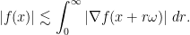
We can average this over all directions 
Switching from polar coordinates back to Cartesian (multiplying and dividing by 

thus 

and the claim follows. (Note that the hypotheses 
Now we handle intermediate cases, when 

for any 

What value of 

averaging over all directions

Thus one is bounding 


and the claim follows.
Remark 27 It is instructive to insert the example in Exercise 21 into the Sobolev embedding theorem. By replacing the
powers of the width
, which is essentially one of the hypotheses in that exercise. Thus, one can view Sobolev embedding as an assertion that the width of a function must always be greater than or comparable to the wavelength scale (the reciprocal of the frequency scale), raised to the power of the dimension; this is a manifestation of the uncertainty principle.
Exercise 28 Let
. Show that the Sobolev endpoint estimate fails in the case
. (Hint: experiment with functions
, where
and equal to one on
.) Conclude in particular that
is not a subset of
, the Sobolev endpoint theorem for
follows from the fundamental theorem of calculus, as mentioned earlier. There are substitutes known for the endpoint Sobolev embedding theorem, but they involve more sophisticated function spaces, such as the space
of spaces of bounded mean oscillation, which we will not discuss here.
The
Exercise 29 (Loomis-Whitney inequality) Let
for some
, and let
be the function
Show that
(Hint: induct on
Lemma 30 (Endpoint Sobolev inequality)
embeds continuously into
.
Proof: It will suffice to show that

for all test functions

and thus

where

From Fubini’s theorem we have
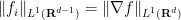
and hence by the Loomis-Whitney inequality

and the claim follows.
Exercise 31 (Connection between Sobolev embedding and isoperimetric inequality) Let
is a smooth
-dimensional manifold. Show that the surface area
of
of
for some constant
depending only on
.) It is also possible to reverse this implication and deduce the endpoint Sobolev embedding theorem from the isoperimetric inequality and the coarea formula, which we will do in later notes.

Exercise 32 Use dimensional analysis to argue why the Sobolev embedding theorem should fail when
. Then create a rigorous counterexample to that theorem in this case.
Exercise 33 Show that
whenever
and
are such that
, and such that at least one of the two inequalities
,
is strict.
Exercise 34 Show that the Sobolev embedding theorem fails whenever
. (Hint: experiment with functions of the form
, where
are widely separated points in space.)
Exercise 35 (Hölder-Sobolev embedding) Let
. Show that
. Use dimensional analysis to justify why one would expect this scaling relationship to arise naturally, and give an example to show that
More generally, with the same assumptions on
, show that
Exercise 36 (Sobolev product theorem, special case) Let
,
, and
be such that
. Show that whenever
, then
, and that
for some constant
depending only on the subscripted parameters. (This is not the most general range of parameters for which this sort of product theorem holds, but it is an instructive special case.)

Exercise 37 Let
. Show that
continuously to
— 3.
It is possible to develop more general Sobolev spaces 
As the theory of singular integrals is beyond the scope of this course, we will illustrate this theory only in the model case 
To explain this, we begin with the Plancherel identity
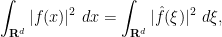
which is valid for all 


for all
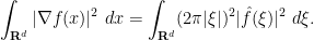
A similar argument then gives
and so on summing in
for all 

Now observe that the quantity 


where we use 


then we see that 
Actually, the two spaces are equal:
Exercise 38 For any
, show that
for all non-negative integers
It is clear that 

It is not hard to verify that this inner product does indeed give 

Being a Hilbert space, 
Exercise 39 (Duality between
and
) Let
. Show also for any continuous linear functional
there exists a unique
such that
for all
is defined via the Fourier transform as
Also show that
for all

The
Exercise 40 (Sobolev embedding for
, show that
. (Hint: use the Fourier inversion formula and the Cauchy-Schwarz inequality.)
Exercise 41 (Sobolev embedding for
, show that
. (Hint: it suffices to handle the extreme case
. For this, first reduce to establishing the bound
to the case when
), and write
for some
Exercise 42 In this exercise we develop a more elementary variant of Sobolev spaces, the
be the space of functions
is finite, where
is the translation of
(with equivalent norms).
- (i) For any
for any
. (Hint: take Fourier transforms and work in frequency space.)
- (ii) Let
. If
, show that one has the equivalence
where we use
. (Hint: To upper bound
for
, express
for
, plus a final term
where
is comparable to
- (iii) If
, show that
as
plus a telescoping series of
, where
The functions


Exercise 43 (Sobolev trace theorem, special case) Let
. For any
where
is the restriction of
. (Hint: Convert everything to

- (i) Show that if
, then
(note that this product has to be defined in the sense of tempered distributions if
is continuous from
for
, and use the preceding cases to estimate the
- (ii) Let
for all
Now we consider a partial converse to Exercise 44.
Exercise 45 (Elliptic regularity) Let
be a constant-coefficient homogeneous differential operator of order
of
We say that
for all
. Thus, for instance, the Laplacian is elliptic. Another example of an elliptic operator is the Cauchy-Riemann operator
in
. On the other hand, the heat operator
, the Schrödinger operator
, and the wave operator
are not elliptic on
.
- (i) Show that if
, then
, and that one has the bound
for some
. (Hint: Once again, rewrite everything in terms of the Fourier transform
of
- (ii) Show that if
- (iii) Let
be a function which is locally in
, then
for every test function


Remark 46 The symbol
of an elliptic operator (with real coefficients) tends to have level sets that resemble ellipsoids, hence the name. In contrast, the symbol of parabolic operators such as the heat operator
has level sets resembling paraboloids, and the symbol of hyperbolic operators such as the wave operator

186 comments
Comments feed for this article
23 February, 2018 at 5:31 am
Sobolev Holder question
Dear Prof. Tao,
is it true that C^s \subset H^s = W^{s,2}? I imagine that it is true but I cannot provide an argument. Thanks in advance.
24 February, 2018 at 8:08 am
Terence Tao
Yes if one has a compact domain, but not in general. One can already see this at the level where the question is whether
  embeds into
  .
.
26 June, 2018 at 7:12 am
Paul Hager
I was confused by the definition “… to be the space of all tempered distributions such that the distribution
  lies in
  …”
…”
A distribution that lies in implicitly means that the distribution is an “ordinary” function?
26 June, 2018 at 11:29 am
Terence Tao
Yes, we view (or more generally,
  ) as a subspace of the space of distributions (see the remarks near Exercise 8 of the previous set of notes).
26 July, 2018 at 10:43 pm
Rajesh
Prof Tao,
“…as the very useful Sobolev embedding theorem, which allows one to trade regularity for integrability…”. Thats the use of Sobolev spaces. In this context, Fourier and Plancheral methods come very handy, when the corresponding Sobolev space is also a Hilbert space. But that is not always the case…. Only L^2 based Sobolev spaces are Hilbert spaces. According to Sobolev emebdding, if the function in R^d need to be holder continuous, then its gardient needs to be L^p integrable with p >= d+1. So for d >1, we need p > 2, so the associated Sobolev space cannot have a Hilbert space structure. So in this context, we cannot use Fourier Plancheral techniques. “But if” (stress If)… I say, that I can always find a Hilbert space, for any d, (even for cases when d>1), how useful a tool that it would be, in the context of PDE. What would the impact be? Any examples of PDE, on which there would be impact? Appreciate your valuable comments…
Thanks and Regards
Rajesh
6 May, 2021 at 3:30 am
Anonymus
Is there any example of a function that is in a sobolev space intersection some gevrey space?
10 August, 2021 at 5:46 pm
Anonymous
I think in exercise 28, phi should be supported in B(2) and identically 1 in B(1) to create a “layer cake”
[Corrected, thanks – T.]
15 March, 2022 at 3:59 pm
Anonymous
At the beginning of the notes, the function and the function
  both have a frequency scale of about
  . Why does the function
  also have a “frequency scale” of about
  ?
?
Don’t we need the periodicity of the sine function as in the previous two examples?
16 March, 2022 at 9:52 am
Terence Tao
The Fourier transform of the function is concentrated in the range
  , which is why one should heuristically think of this function as having a frequency scale of
  . Alternatively, this function has a “wavelength” of
  (albeit with only one oscillation of this wavelength being present, rather than many), and frequency is inversely proportional to wavelength.
16 March, 2022 at 11:01 am
J
Why in the function ,
,  is not considered as the “width” of
  as for instance Example 4 does?
[I’m sorry, I was not able to parse this question. -T]
16 March, 2022 at 1:00 pm
J
Sorry, I meant to say *Exercise* 4. In that exercise, the function is said to have “width”
  . So I was wondering if one should also say that the function
  has with
  , where you interprets
  as the frequency scale.
16 March, 2022 at 2:14 pm
Terence Tao
Yes, the function would informally have frequency
  , wavelength
  , amplitude
  , and width
  , and consist of
  oscillations. Drawing a graph of this function should make these statistics clear.
16 March, 2022 at 10:58 am
Anonymous
In Exercise 4, whenever one differentiates the function once, one has a factor of and
and  ; so by the assumption on
  , it is bounded by totally one factor of
  . Since
  , so all
  ,
,  , are dominated by
  . On the other hand, the constant
  comes from the max of
  ,
,  .
.
How would you organize a neat formal argument? The higher-order mixed partial derivatives are messy. Even if one focuses on the case when , more and more terms appear by the product rule as
  increases.
16 March, 2022 at 12:32 pm
Terence Tao
An induction on would work here. (Here one has to invest a little bit of thought into developing a suitable induction hypothesis. For instance, it would be good to have the induction hypothesis cover both the sine and cosine cases.)
16 March, 2022 at 12:54 pm
J
It is said in the notes that
 are designed to “fill up the gaps” between the discrete spectrum
  of the continuously differentiable spaces.
The Hölder spaces
Exercise 8 seems to suggest that the gaps are not perfectly filled up yet:

Is there a family of spaces filling the gaps between and
and  ?
?
16 March, 2022 at 1:17 pm
J
As before,
I think you want to switch and
and  if they are meant to be consistent with Exercise 6.
[Corrected, thanks – T.]
16 March, 2022 at 1:47 pm
J
As Exercise 10 and 11 show, the Holder spaces do not fill the gaps between and
and  completely.
One may want to make some kind of room of argument for
  so that one can conclude something for
  . But this does not work because of the gaps. (Perhaps this is not how the Holder spaces are supposed to be used at all.)
Naively, one can simply assume stronger differentiability when needed. How much more flexibility does one gain if one has already at least the regularity of, say, by using
  instead of simply
  ?
?
16 March, 2022 at 4:06 pm
Terence Tao
If one really wants to work with a continuum of spaces that does not experience discontinuities at integer regularities, then one can work with Holder-Zygmund spaces (a special type of Besov space), which agree with the Holder spaces
  when
when  and
and  but disagree with the classical spaces
  when
when  . These are discussed for instance in Stein’s “Singular integrals and differentiability properties of functions”.
In elliptic and parabolic PDE one often expends significant effort to improve the regularity of a solution from some “critical” regularity (which for instance could be ) to a slightly “subcritical” regularity, such as
  ; this is often non-trivial and uses tools such as Moser iteration. Once one has some subcritical regularity, though, it is often relatively easy to gain even more regularity.
even more regularity.
16 March, 2022 at 2:12 pm
J
Can one use Lemma 23 to define the Sobolev spaces, i.e., completion of the space of test functions with respect to the Sobolev norm ? Then one would have Lemma 23 for free; would this make other originally “easy” propositions more difficult to prove?
16 March, 2022 at 4:23 pm
Terence Tao
Yes, this is an alternate route to setting up the foundations of the theory; Definition 18 will now need to be a theorem, rather than a definition, but one ends up in the same place at the end. (The situation is more delicate in the presence of a boundary; cf. the comments after Exercise 13.)
16 February, 2023 at 6:32 am
Anonymous
At the beginning of the discussion of Sobolev embeddings, is the fact that is a subset of
  a consequence of the inequality (1) or something one assumes true when proving the inclusion map from
  to
to  is continuous?
16 February, 2023 at 9:59 am
Anonymous
Inequality (1) shows is a subset of
  .
.
19 February, 2023 at 5:06 am
Anonymous
1. One first establishes the inequality (1) for . If
. If  , Lemma 23 shows
  in
in  for some sequence
  . The inequality (1) (for
  )shows that
  is a Cauchy sequence in
  and by completeness,
  converges to some
  in
in  . The uniqueness of limits in the sense of distributions implies that
  and one thus shows (1) for every
  , which implies
  . Does this argument work?
2. It seems that one does not need to use the fact that is the dual space of
  as in:
“Also, since is the dual space of
  , the distributional limit of any sequence bounded in
  remains in
  “.
“.
(One way to show completeness of is to use duality, though.)
16 January, 2024 at 11:20 am
Anonymous
Maybe I am missing something but is the first part of exercise 11 right, with ,
,  , and
, and  ?
?  is not continuously differentiable at 0. So let
  be constant near
  . Then
  is not in
  , right?
[Oops, one should exclude the endpoints here, now corrected. -T]