
Suppose we have a large number of scalar random variables 


The basic intuition here is that it is difficult for a large number of independent variables 
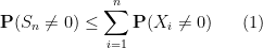
There are many applications of the concentration of measure phenomenon, but we will focus on a specific application which is useful in the random matrix theory topics we will be studying, namely on controlling the behaviour of random 
Once one has a sufficient amount of independence, the concentration of measure tends to be sub-gaussian in nature; thus the probability that one is at least 


This is only a brief introduction to the concentration of measure phenomenon. A systematic study of this topic can be found in this book by Ledoux.
— 1. Linear combinations, and the moment method —
We begin with the simple setting of studying a sum
In this section we shall concern ourselves primarily with bounded random variables; in the next section we describe the basic truncation method that can allow us to extend from the bounded case to the unbounded case (assuming suitable decay hypotheses).
The zeroth moment method gives a crude upper bound when 
but in most cases this bound is worse than the trivial bound 
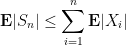
The first moment method is somewhat better, giving the bound
which when combined with Markov’s inequality gives the rather weak large deviation inequality

As weak as this bound is, this bound is sometimes sharp. For instance, if the 


Informally, one can view (2) as the assertion that 
The first moment method also shows that
and so we can normalise out the means using the identity

Replacing the 

Now we consider what the second moment method gives us. We square

If we assume that the 


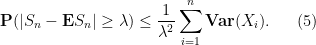
which when combined with Chebyshev’s inequality (and the mean zero normalisation) yields the large deviation inequality

Without the normalisation that the
Informally, this is the assertion that 
The inequality (5) is sharp in two ways. Firstly, we cannot expect any significant concentration in any range narrower than the standard deviation 


Now we turn to higher moments. Let us assume that the 


Let us also assume that the 


To compute the expectation of the product, we can use the 


where 


We are now faced with the purely combinatorial problem of estimating 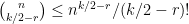

which after using a crude form 

and so
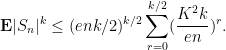
If we make the mild assumption
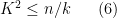
then from the geometric series formula we conclude that

(say), which leads to the large deviation inequality

This should be compared with (2), (5). As 
Remark 1 Note how it was important here that
, can be estimated, but due to the lack of the absolute value sign, these moments do not give much usable control on the distribution of the
(which can easily be made explicit, but we will not do so here).
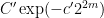
Now suppose that the 

for some absolute constants 


By using Stirling’s formula (Exercise 2 from Notes 0a) one can show that the quadratic decay in (8) cannot be improved; see Exercise 2 below.
It was a little complicated to manage such large moments 
Lemma 1 (Hoeffding’s lemma) Let
be a scalar variable taking values in an interval
. Then for any
,


Proof: It suffices to prove the first inequality, as the second then follows using the bound 
By subtracting the mean from 


which on taking expectations gives

and the claim follows.

Exercise 1 Show that the
factor in (10) can be replaced with
, and that this is sharp. (Hint: use Jensen’s inequality.)
We now have the fundamental Chernoff bound:
Theorem 2 (Chernoff inequality) Let
and variance
. Then for any
, one has
for some absolute constants
and
.

Proof: By taking real and imaginary parts we may assume that the 


(with slightly different constants 
To do this, we shall first compute the exponential moments

where 

To compute 


Thus we have

and thus by Markov’s inequality

If we optimise this in
Informally, the Chernoff inequality asserts that 
Exercise 2 Let
be fixed independently of
, thus
and
, and so
and
. Using Stirling’s formula (Notes 0a), show that
for some absolute constants
. What happens when
?

Exercise 3 Show that the term
in (11) can be replaced with
(which is superior when
). (Hint: Allow
Exercise 4 (Hoeffding’s inequality) Let
, and let
. Show that one has
for some absolute constants
.

Remark 2 As we can see, the exponential moment method is very slick compared to the power moment method. Unfortunately, due to its reliance on the identity
, this method relies very strongly on commutativity of the underlying variables, and as such will not be as useful when dealing with noncommutative random variables, and in particular with random matrices. Nevertheless, we will still be able to apply the Chernoff bound to good effect to various components of random matrices, such as rows or columns of such matrices.
The full assumption of joint independence is not completely necessary for Chernoff-type bounds to be present. It suffices to have a martingale difference sequence, in which each 
Theorem 3 (Azuma’s inequality) Let
almost surely. Assume also that we have the martingale difference property
almost surely for all
(here we assume the existence of a suitable disintegration in order to define the conditional expectation, though in fact it is possible to state and prove Azuma’s inequality without this disintegration). Then for any
for some absolute constants


A typical example of 

Proof: Again, we can reduce to the case when the

Note that 

Once again, we consider the exponential moment 

We do not have independence between 


The quantity 

Applying (10) to the conditional expectation, we have

and

Iterating this argument gives

and thus by Markov’s inequality

Optimising in
Exercise 5 Suppose we replace the hypothesis
for some scalars
. Show that we still have (13), but with
.
Remark 3 The exponential moment method is also used frequently in harmonic analysis to deal with lacunary exponential sums, or sums involving Radamacher functions (which are the analogue of lacunary exponential sums for characteristic
). Examples here include Khintchine’s inequality (and the closely related Kahane’s inequality). The exponential moment method also combines very well with log-Sobolev inequalities, as we shall see below (basically because the logarithm inverts the exponential), as well as with the closely related hypercontractivity inequalities.
— 2. The truncation method —
To summarise the discussion so far, we have identified a number of large deviation inequalities to control a sum 
- The zeroth moment method bound (1), which requires no moment assumptions on the
- The first moment method bound (2), which only requires absolute integrability on the
- The second moment method bound (5), which requires second moment and pairwise independence bounds on
- Higher moment bounds (7), which require boundedness and
- Exponential moment bounds such as (11) or (13), which require boundedness and joint independence (or martingale behaviour), and give quadratic-exponential decay in
We thus see that the bounds with the strongest decay in 


is the restriction of 

is the complementary event. One can similarly split 

and

The idea is then to estimate the tail of 


Let us begin with a simple application of this method.
Theorem 4 (Weak law of large numbers) Let
be iid scalar random variables with
for all
, where
converges in probability to
.
Proof: By subtracting 

If 


(where the rate of decay here depends on 


But by the dominated convergence theorem (or monotone convergence theorem), we may make 


since 
A more sophisticated variant of this argument (which I gave in this earlier blog post, which also has some further discussion and details) gives
Theorem 5 (Strong law of large numbers) Let
Proof: We may assume without loss of generality that
Next, we apply a sparsification trick. Let 


Fix 


for some 

summing, we conclude

Applying the Borel-Cantelli lemma (Exercise 1 from Notes 0), we see that we will be done as long as we can choose
and
are both finite. But this can be accomplished by setting 


To give another illustration of the truncation method, we extend a version of the Chernoff bound to the subgaussian case.
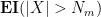
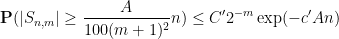
Proposition 6 Let
be iid copies of a subgaussian random variable
for all
. Let
(independent of
for some constants
depending on
. Furthermore,
grows linearly in
.


Proof: By subtracting the mean from 

where 


where 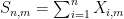

(say). Each 


(say) for some
Exercise 6 Show that the hypothesis that
is independent of
Exercise 7 Show that the subgaussian hypothesis can be generalised to a sub-exponential tail hypothesis
provided that
. Show that the result also extends to the case
, except with the exponent
replaced by
for some
(say) is already as large as
.)

— 3. Lipschitz combinations —
In the preceding discussion, we had only considered the linear combination 

Theorem 7 (McDiarmid’s inequality) Let
, and let
be a function with the property that if one freezes all but the
for some
, then
for all
,
for
for some absolute constants
.


Proof: We may assume that

To compute this quantity, we again use the exponential moment method. Let 
To compute this, let us condition

We can simplify this as

where

For 


Integrating out the conditioning, we see that we have upper bounded (16) by

We observe that 


which we rearrange as

and thus by Markov’s inequality

Optimising in
Exercise 8 Show that McDiarmid’s inequality implies Hoeffding’s inequality (Exercise 4).
Remark 4 One can view McDiarmid’s inequality as a tensorisation of Hoeffding’s lemma, as it leverages the latter lemma for a single random variable to establish an analogous result for
The most powerful concentration of measure results, though, do not just exploit Lipschitz type behaviour in each individual variable, but joint Lipschitz behaviour. Let us first give a classical instance of this, in the special case when the
Exercise 9 Let
, and let
be real constants. Show that
is a real gaussian with mean
and variance
.
Show that the same claims also hold with complex gaussians and complex constants
.
Exercise 10 (Rotation invariance) Let
be an
-valued random variable, where
are iid real gaussians. Show that for any orthogonal matrix
,
.
Show that the same claim holds for complex gaussians (so
-valued), and with the orthogonal group
.
Theorem 8 (Gaussian concentration inequality for Lipschitz functions) Let
be a
for all
, where we use the Euclidean metric on
for some absolute constants

Proof: We use the following elegant argument of Maurey and Pisier. By subtracting a constant from 

By smoothing
for all 
Once again, we use the exponential moment method. It will suffice to show that

for some constant 
To exploit the Lipschitz nature of 
and thus (by independence of

It is tempting to use the fundamental theorem of calculus along a line segment,

to estimate 
The reason for this is that 
To exploit this, we first use Jensen’s inequality to bound

Applying the chain rule and taking expectations, we have

Let us condition 


for some absolute constant
Exercise 11 Show that Theorem 8 is equivalent to the inequality
holding for all
is the

Now we give a powerful concentration inequality of Talagrand, which we will rely heavily on later in this course.
Theorem 9 (Talagrand concentration inequality) Let
, and let
be a
for the purposes of defining “Lipschitz” and “convex”). Then for any
for some absolute constants
is a median of


We now prove the theorem, following the remarkable argument of Talagrand.
By dividing through by 


for any convex set 


for any 


which then gives (19).
We would like to establish (20) by induction on dimension 


Lemma 10 (Combinatorial distance controls Euclidean distance) Let
.
Proof: Suppose 


Thus to show (20) it suffices (after a modification of the constant
We first verify the one-dimensional case. In this case, 

Now suppose that 


Lemma 11 For any
, we have

Proof: Observe that 


Let us now freeze
Using the above lemma (with some

applying Hölder’s inequality and the induction hypothesis (21), we can bound this by
which we can rearrange as

where 


which can be verified by elementary calculus if 

Taking expectations in

Using the inequality 

The above argument was elementary, but rather “magical” in nature. Let us now give a somewhat different argument of Ledoux, based on log-Sobolev inequalities, which gives the upper tail bound

but curiously does not give the lower tail bound. (The situation is not symmetric, due to the convexity hypothesis on
Once again we can normalise
Lemma 12 (Log-Sobolev inequality) Let
for some absolute constant

Remark 5 If one sets
and normalises
, this inequality becomes
which more closely resembles the classical log-Sobolev inequality of Gross. The constant

Proof: We first establish the

From Jensen’s inequality, 

From convexity of 


and

when 

in this case. Similarly when 
To show the general case, we induct on 

where 

From the convexity of 


Now, by the chain rule

where 


Inserting this into (23), (24) we close the induction.
Now let 

setting 

which we can rewrite as

From Taylor expansion we see that
as 

for any

By Markov’s inequality, we conclude that

optimising in
Remark 6 The same argument, starting with Gross’s log-Sobolev inequality for the gaussian measure, gives the upper tail component of Theorem 8, with no convexity hypothesis on
, and so one obtains the lower tail component as well. The method of obtaining concentration inequalities from log-Sobolev inequalities (or related inequalities, such as Poincaré-type ienqualities) by combining the latter with the exponential moment method is known as Herbst’s argument, and can be used to establish a number of other functional inequalities of interest.
We now close with a simple corollary of the Talagrand concentration inequality, which will be extremely useful in the sequel.
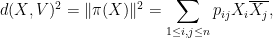
Corollary 13 (Distance between random vector and a subspace) Let
be a subspace of
. Then for any
for some absolute constants

Informally, this corollary asserts that the distance between a random vector 
Proof: The function 

To finish the argument, it then suffices to show that

We begin with a second moment calculation. Observe that
where 


where the latter follows by representing 

where 


where the latter bound comes from representing 


127 comments
Comments feed for this article
14 November, 2013 at 10:57 pm
Anonymous
Are the summands for last applicational result really independent or merely uncorrelated?
[Corrected, thanks – T.]
24 October, 2014 at 12:26 am
Anonymous
Do you want the variance to be “at least 1” or “at most 1”. The current formulation seems inconsistent with the note right after this line.
[“At most”. Note clarified to remove the confusion. -T.]
20 September, 2015 at 10:11 am
Entropy and rare events | What's new
[…] inequality, but there are of course many other estimates of this type (see e.g. this previous blog post for some others). Roughly speaking, concentration of measure inequalities allow one to make […]
21 September, 2015 at 1:22 pm
Jiasen Yang
Dear Professor Tao,
Thank you for the detailed post! I’ve been going through the proof of McDiarmid’s inequality, and I don’t see why it is necessary to assume that the ‘s are independent. I wonder if you could point out which step(s) I missed?
Thanks very much!
[One needs the independence to ensure that (say) continues to have mean zero even after conditioning on
  . -T. Note also that the theorem fails quite badly if for instance one has the very strong coupling
 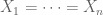 . -T.]
21 September, 2015 at 7:23 pm
Jiasen Yang
Dear Professor Tao,
Thank you for your timely reply! Your coupling argument certainly makes sense, but I’m still having trouble determining which step of the proof uses independence directly. Following your point, I agree that $E[X_n] \neq E[X_n|X_1,\ldots,X_{n-1}]$ in general, but I don’t see where $X_n$ is assumed to have mean zero?
Actually, my question originally arose as I was reading a paper which claims to use McDiarmid’s inequality for dependent $X_i$’s after replacing the assumption
$$ |F(x_1,\ldots,x_{i-1},x_i,x_{i+1},\ldots,x_n) – F(x_1,\ldots,x_{i-1},x_i’,x_{i+1},\ldots,x_n)| \leq c_i $$
by
$$ |\bf{E}[f(X)|x_1,\ldots, x_{i-1},x_i] – \bf{E}[f(X)|x_1,\ldots, x_{i-1},x_i’]| \le c_i $$, but I don’t see why this new assumption resolves the issue.
Thank you again, and please forgive me for my stubbornness!
21 September, 2015 at 7:39 pm
Terence Tao
Sorry, my previous reply was quite incorrect, I was thinking of a different concentration equality. For McDiarmid, the claim that the conditioned function obeys the same hypotheses as the original function
  requires the independence hypothesis, as one will find if one expands out the proof of this claim.
21 September, 2015 at 8:08 pm
Jiasen Yang
Ah! I finally see your point. Thank you Professor!
23 October, 2015 at 8:06 am
275A, Notes 3: The weak and strong law of large numbers | What's new
[…] theory and high dimensional geometry. We will not discuss these topics much in this course, but see this previous blog post for some further […]
6 November, 2015 at 4:19 pm
Mahmood
Dear Professor Tao,
In the proof of Lemma 11 and the definition of set . What happens if such
  is equal to
  ? Is it still valid to say that
  . For example, when the set
  has the points whose
  coordinates are all equal to
  , then
  does not have any element with the last coordinate 1. Am I missing something?
Thanks.
6 November, 2015 at 9:46 pm
Terence Tao
Oops, you’re right, the case has to be handled separately, but the bound is better in that case (one can stay in the
  slice). I’ve updated the argument accordingly.
7 November, 2015 at 8:51 am
mazrouei
Thanks for your reply.
19 November, 2015 at 2:51 pm
275A, Notes 5: Variants of the central limit theorem | What's new
[…] in which the underlying random variable is not bounded, but enjoys good moment bounds. See this previous blog post for these inequalities and some further discussion. Last, but certainly not least, there is an […]
17 February, 2016 at 6:59 pm
Anonymous
Hello Professor Tao,
In the proof of SLLN, I am not sure what do you mean by ‘countable additivity’ in building the connections bewteen convergence of two sequences. Does it mean adding O(\varepsilon)?
Thanks!
Jack
17 February, 2016 at 7:22 pm
Terence Tao
If is almost surely convergent to
  , then almost surely it is the case that
  fluctuates by at most
  around
  (in the sense that the limit superior and limit inferior are both almost surely
  . Setting
  (say) for
  and using countable additivity (which implies that the countable intersection of almost sure events is still almost sure, we conclude that the limit superior and limit inferior are both almost surely
  , giving the SLLN.
17 February, 2016 at 8:33 pm
Anonymous
Ah, I see. Thanks a lot for your reply!
Best,
Jack
9 April, 2016 at 7:44 am
Anonymous
Dear Prof. Tao, I believe your notes are just impressive.
What can we say on the lower bound on $Pr[|S_n|\geq \lambda]\geq ?$,depending on the moments of the distribution of the jointly independent, zero mean, variables $X_i$?
11 April, 2016 at 8:50 am
Terence Tao
This is the realm of large deviation theory; these bounds tend to depend in various subtle ways on the precise distribution of the independent variables. See for instance this paper of Nagaev for a classical survey of results; probably there are more up to date surveys also.
14 April, 2016 at 10:39 am
gninrepoli
I think that the probability of a recursive nature, so this phenomenon is possible. Probability – it’s just part of the recursion. Any probabilistic model is necessary to approximate recursion, which we can control. For example the set of prime numbers is recursive. But how to prove it.
25 April, 2016 at 3:24 pm
Nathan
Dear Prof. Tao,
First I would like to thank you for your notes, which are quite impressive!
I do not understand why each summand has a variance of in the computation of the variance of
  (corollary 13). Since
  and a term in the computation has the form
 ![E[X_i^2X_j^2]](https://s0.wp.com/latex.php?latex=E%5BX_i%5E2X_j%5E2%5D&bg=ffffff&fg=545454&s=0&c=20201002) , shouldn’t we have an
, shouldn’t we have an  ?
?
Thanks!
26 April, 2016 at 8:34 am
Terence Tao
26 April, 2016 at 11:27 am
Nathan
Thank you!
2 March, 2017 at 12:17 am
keej
I was also stuck on this point; thanks for clarifying!
5 June, 2016 at 4:49 am
Vaibhav
Hi Prof. Terrence Tao,
I am a very simple question. In, (McDiarmid’s inequality) it is not clear how does it depend upon N, the number of random variables concerned. Intuitively, and as you mention elsewhere, the inequality should become stronger. That is, as the number of random variables increase, the deviation from the mean of the function should be less likely. Could you kindly clarify.
Quoting you:
“The basic intuition here is that it is difficult for a large number of independent variables {X_1,\ldots,X_n} to “work together” to simultaneously pull a sum {X_1+\ldots+X_n} or a more general combination {F(X_1,\ldots,X_n)} too far away from its mean. Independence here is the key; concentration of measure results typically fail if the {X_i} are too highly correlated with each other.”
I fail to see this effect.
6 June, 2016 at 1:53 pm
Terence Tao
Let’s say we are working in the normalisation . The hypothesis of Theorem 7 allows
  to range over an interval of size
  ; but McDiarmid’s inequality shows that concentration instead occurs at a shorter interval at the scale of
  .
.
6 June, 2016 at 6:19 pm
Vaibhav
Dear Prof. Tao, Thanks a lot. This helps most certainly.
6 June, 2016 at 6:51 pm
Vaibhav
Dear Prof. Tao,
I had a following question about Levy’s Lemma (another celebreated concentration of measure result).
First the Levy’s Lemma.
Let $f : S^k \rightarrow R$
be a function with Lipschitz constant $\eta$ (with respect to the Euclidean norm) and $X \in k$
and a point $X \in S^{k}$ be chosen uniformly at random. Then
\begin{align}
\label{levy}
Pr\{|f(X) – \bar{f}| > \alpha\}\le exp (-C(k+1)\alpha^{2}/\eta^2 )
\end{align}
for some constant $C >0$ and $\bar{f}$ is the mean value of the function over the sphere.
Now, here is my question: This Lemma seems to hold for a point chosen
uniformly at random over a sphere.
My question is….suppose I choose a point on an N dimensional sphere (X_1, X_2,…, X_N) such that (X_1^2, X_2^2, …, X_N^2) is chosen from a uniform distribution.
Certainly (X_1^2, X_2^2, …, X_N^2) chosen from a uniform distribution does not imply (X_1, X_2,…, X_N) will be a uniformly random point on the sphere.
But intuitively, I will expect Levy’s Lemma (or say a weaker version) to hold as I expect it to hold
for almost all points on the sphere.
My computer simulations also show this to be the case.
But, I cannot make mathematical arguments to justify my intuition and my simulations.
Best,
vaibhav
Ps: If I can show this, I can show a neat result in evolutionary biology, which I will be happy to show it to you if you would like.
Many thanks to you!
28 June, 2016 at 5:41 am
Ahn
Dear prof. Tao,
While I read the proof of proposition 6, I could not follow the step at the end where you applied chernoff bound. For example, what did you choose for lambda?
I would appreciate your help.
29 June, 2016 at 6:51 am
Terence Tao
There is a lot of latitude here in what to choose for , for instance one can take
  for some small
  . Note that the bound on the RHS is not optimal, but suffices for the application at hand.
8 November, 2016 at 8:40 am
Fast Randomized SVD – Facebook Research
[…] our approximation by appealing to concentration of measure results for random matrices – see Terry Tao’s lecture notes on the topic for some useful […]
12 February, 2017 at 11:53 am
keej
Could anyone please explain why in the proof of Hoeffding’s lemma, the first Taylor expansion is and not just the naive
  ?
?
12 February, 2017 at 3:39 pm
Anonymous
The simpler estimate for the remainder term applies only for bounded
  .
.
12 February, 2017 at 5:01 pm
keej
Of course, thank you.
13 May, 2017 at 5:28 pm
Zahra
Hello Prof. Tao,
Any known results for the extension of theorem 8 to the case when be a vector of iid sub-gaussian variables? Many Thanks.
[Probably. I don’t have references handy, but I would recommend checking Ledoux’s book on the subject. -T.]
22 May, 2017 at 5:55 pm
Quantitative continuity estimates | What's new
[…] is the proof by Maurey and Pisier of the gaussian concentration inequality, given in Theorem 8 of this previous blog post. In a similar vein, if one wishes to compare a scalar random variable of mean zero and variance […]
24 December, 2017 at 1:19 pm
AL Ray
I don’t understand something in the proof of the Lemma 10 why is and not
  ?
?
Thanks in advance!
[This is a typo, now fixed – T.]
30 December, 2017 at 10:41 pm
Tim
Dear Prof. Tao,
Thanks for the insightful notes. I have two questions:
1. When calculating the variance of d(X, V)^2, a term in the computation will be E[X_i^2 X_j^2], which I think should be 1 instead of O(K^2) since X_i and X_j are independent.
2. Are there any more direct ways to calculate / estimate the expectation of d(X, V)?
Thanks in advance!
31 December, 2017 at 10:29 am
Terence Tao
It’s true one can improve the bound on the variance of , but unfortunately this does not significantly improve the concentration bound because of the uncertainty of
  coming from the use of Theorem 9.
I don’t know of much sharper ways to control the expectation, but there are several routes to the concentration property at least, starting with the classic work of Hanson and Wright.
12 November, 2019 at 6:47 pm
254A, Notes 9 – second moment and entropy methods | What's new
[…] random variable will concentrate around its mean if its variance is not too large. See these previous notes for more discussion of the concentration of measure phenomenon. One can often obtain stronger […]
27 June, 2020 at 8:43 pm
Yijia Liu
I have been trying to work out the computations for the final part of proposition 6 but I couldnt get the 2^-m factor.
From https://math.stackexchange.com/questions/3734229/chernoff-bound-for-sum-of-sub-gaussian-variables-via-truncation-method it seems that we cannot replace $1/100(m+1)^2$ with $2^{-m-1}$. Is this a typo or have I missed something in calculations.
[Corrected, thanks – T.]
11 October, 2021 at 9:19 am
254A, Supplement 4: Probabilistic models and heuristics for the primes (optional) | What's new
[…] above claim using concentration of measure results such as the Chernoff inequality, as discussed in this previous blog post. The estimate (2) reflects the general heuristic of expected square root cancellation: when summing […]
6 November, 2021 at 10:49 am
Alan Chang
In the proof of Theorem 8, should (all five instances of) be
be  ?
?
[Corrected, thanks – T.]
7 April, 2022 at 6:42 am
Matteo Russo
Dear Prof.Tao,
Upon thanking you for the notes, I would like to ask whether Talagrand’s Inequality held even in the case where 1-Lipschitz is with respect to the l1-norm. If not, what type of concentration guarantees could still be claimed?
Thanks in advance!
7 April, 2022 at 11:17 am
Terence Tao
The standard concentration inequality that is used in such settings is McDiarmid’s inequality.
18 May, 2023 at 9:39 pm
David Roberts
I suspect there’s a (minor) typo in the proof of the Chernoff inequality (Theorem 2). After “we use the hypothesis that and (9) to obtain” there’s an equation, following from the previous display which is an inequality.
And on the conclusion of the proof of that theorem, I suspect that the of the two exponentials comes from an asymmetry in the tails. At least, This is the case in a proof of a special case (sums of arbitrary Bernoulli RVs) I’ve seen in one treatment elsewhere. But I’ve not seen other proofs give an upper bound of this form, in my limit searching.
One thing which I haven’t been able to justify to myself is why you consider the parameter in that proof to be bounded above by 1. Is it somehow due to implicitly needing to consider something like keeping a factor of
  positive, while at the same time keeping
  positive, to use in a previous estimate?
19 May, 2023 at 12:32 am
David Roberts
Sorry, one more thought: might the bound on come from needing
  to still be bounded by 1? Just casting about at this point.
20 May, 2023 at 1:34 pm
Terence Tao
Typo now corrected. The condition is needed to be able to estimate the
  term in (9) by
  , which allows one to bound the entire RHS of (9) by
  .
.
20 May, 2023 at 3:32 pm
David Roberts
Oh, excellent, thanks.