This week at UCLA, Pierre-Louis Lions gave one of this year’s Distinguished Lecture Series, on the topic of mean field games. These are a relatively novel class of systems of partial differential equations, that are used to understand the behaviour of multiple agents each individually trying to optimise their position in space and time, but with their preferences being partly determined by the choices of all the other agents, in the asymptotic limit when the number of agents goes to infinity. A good example here is that of traffic congestion: as a first approximation, each agent wishes to get from A to B in the shortest path possible, but the speed at which one can travel depends on the density of other agents in the area. A more light-hearted example is that of a Mexican wave (or audience wave), which can be modeled by a system of this type, in which each agent chooses to stand, sit, or be in an intermediate position based on his or her comfort level, and also on the position of nearby agents.
Under some assumptions, mean field games can be expressed as a coupled system of two equations, a Fokker-Planck type equation evolving forward in time that governs the evolution of the density function  of the agents, and a Hamilton-Jacobi (or Hamilton-Jacobi-Bellman) type equation evolving backward in time that governs the computation of the optimal path for each agent. The combination of both forward propagation and backward propagation in time creates some unusual “elliptic” phenomena in the time variable that is not seen in more conventional evolution equations. For instance, for Mexican waves, this model predicts that such waves only form for stadiums exceeding a certain minimum size (and this phenomenon has apparently been confirmed experimentally!).
Due to lack of time and preparation, I was not able to transcribe Lions’ lectures in full detail; but I thought I would describe here a heuristic derivation of the mean field game equations, and mention some of the results that Lions and his co-authors have been working on. (Video of a related series of lectures (in French) by Lions on this topic at the Collége de France is available here.)
To avoid (rather important) technical issues, I will work at a heuristic level only, ignoring issues of smoothness, convergence, existence and uniqueness, etc.
— 1. Hamilton-Jacobi-Bellman equations —
Before considering mean field games, let us consider a more classical problem in calculus of variations, namely that of a single agent trying to optimise his or her path in spacetime with respect to a fixed cost function to minimise against. (One could also reverse the sign here, and maximise a utility function rather than minimise a cost function; mathematically, there is no distinction between the two. (A half-empty glass is mathematically equivalent to a half-full one.))
Specifically, suppose that an agent is at some location  at time
  in some ambient domain (which, for simplicity, we shall take to be a Euclidean space
  ), and would like to end up at some better location
  at a later time
  . To model this, we imagine that each location
  in the domain has some cost
  at this final time
  , which is small when is a desirable location and large otherwise, so that the agent would like to minimise
  . (In the traffic problem, one may wish to be at a given location
  by time , or failing that, on some location close to , or perhaps at some secondary backup location in case is too inaccessible due to traffic; so the cost function may have a global minimum at but perhaps also have local minima elsewhere.)
If transportation was not a problem, this is an easy problem to solve: one simply finds the value of that minimises  , and the agent takes an arbitrary path (e.g. a constant velocity straight line path) from at time to at time
  .
.
But now suppose that there is a transportation cost in addition to the cost of the final location – for instance, moving at too fast a velocity may incur an energy cost. To model this, we introduce a velocity cost function  , where
  measures the marginal cost of moving at a given velocity
  for time
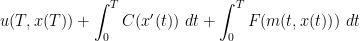
  , and then define the total cost of a trajectory
 ![{x: [0,T] \rightarrow {\bf R}^d}](https://s0.wp.com/latex.php?latex=%7Bx%3A+%5B0%2CT%5D+%5Crightarrow+%7B%5Cbf+R%7D%5Ed%7D&bg=ffffff&fg=000000&s=0&c=20201002) by the formula
by the formula

The goal now is to select a trajectory that minimises this total cost. This is a simplified model, in which cost depends only on velocity and not on position and time; one could certainly consider more complicated cost functions  which depend on these parameters, in which case the
  term above would have to be replaced with
  , but let us work with the above simplified model for the current discussion.
A model example of a cost function  is a quadratic cost function
  (other normalising factors than
  can of course be used here). Thus one is penalised for moving too fast, or for “wasting” velocity by zig-zagging back and forth. In such a situation, the agent should move in a straight line at constant velocity to a location with relatively low final cost but which is also reasonably close to the original position ; the global minimum for the final cost
  may no longer be the best place to shoot for, as it may be so far away that the transportation cost exceeds whatever cost savings one gets from the final cost.
More generally, it is natural to choose to be convex – thus, for instance, given two velocities and  ,
,  should be less than or equal to the average of
  and
and  . The reason for this is that one can effectively “simulate” a velocity of
  by zig-zagging between velocities and velocities , and so (assuming infinite maneuverability) one can always travel at an effective velocity of at a mean cost of
  .
.
To avoid some technical issues, we will assume to be strictly convex, and to make the formulae slightly nicer we will also assume that is even, thus  .
.
One way to compute the optimal trajectory here is to solve the Euler-Lagrange equation associated to (1), with the boundary condition that the initial position is fixed. This is an ODE for  which can be solved by a variety of methods. But there is another approach, based on solving a PDE rather than an ODE, and which conveys more information about the solution (such as the dependence on the initial position). The idea is to generalise the initial time from
  to any other time
  between and . More precisely, given any
  and
and  , define the optimal cost
  at the point
  in spacetime to be the infimum of the cost

over all (smooth) paths ![{x: [t_0,T] \rightarrow {\bf R}^d}](https://s0.wp.com/latex.php?latex=%7Bx%3A+%5Bt_0%2CT%5D+%5Crightarrow+%7B%5Cbf+R%7D%5Ed%7D&bg=ffffff&fg=000000&s=0&c=20201002) starting at
starting at  and with an arbitrary endpoint . Informally, this is the cost the agent would place on being at position
  at time .
By definition, when  , the optimal cost at coincides with the final cost at , which justifies using the same symbol to denote both. The final cost
  can thus be viewed as a boundary condition for the optimal cost.
But what happens for times less than ? It turns out that (under some regularity hypotheses, which I will not discuss here) the optimal cost function obeys a partial differential equation, known as the Hamilton-Jacobi-Bellman equation, which we shall heuristically derive (using infinitesimals as an informal tool) as follows.
Imagine that the agent finds herself or himself at position at some time  , and is deciding where to go next. Presumably there is some optimal velocity in which the agent should move in (a priori, this velocity need not be unique). So, if is an infinitesimal time, the agent should move at this velocity for time , ending up at a new position
  at time
  , and incurring a travel cost of . At this point, the optimal cost for the remainder of the agent’s journey is given by
  , by definition of . This leads to the heuristic formula

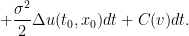
which on Taylor expansion (and omitting higher order terms) gives
![\displaystyle u(t_0,x_0) = u(t_0,x_0) + dt [ \partial_t u(t_0,x_0) + v \cdot \nabla_x u(t_0,x_0) + C(v) ].](https://s0.wp.com/latex.php?latex=%5Cdisplaystyle++u%28t_0%2Cx_0%29+%3D+u%28t_0%2Cx_0%29+%2B+dt+%5B+%5Cpartial_t+u%28t_0%2Cx_0%29+%2B+v+%5Ccdot+%5Cnabla_x+u%28t_0%2Cx_0%29+%2B+C%28v%29+%5D.&bg=ffffff&fg=000000&s=0&c=20201002)
On the other hand, is being chosen to minimise the final cost. Thus we see that should be chosen to minimise the expression

Note from the strict convexity that this minimum will be unique, and will be some function of  . If we introduce the Legendre transform
  of by the formula
then the minimal value of  is just
  (here we use the hypothesis that is even). We conclude that
![\displaystyle u(t_0,x_0) = u(t_0,x_0) + dt [ \partial_t u(t_0,x_0) - H(\nabla_x u(t_0,x_0)]](https://s0.wp.com/latex.php?latex=%5Cdisplaystyle++u%28t_0%2Cx_0%29+%3D+u%28t_0%2Cx_0%29+%2B+dt+%5B+%5Cpartial_t+u%28t_0%2Cx_0%29+-+H%28%5Cnabla_x+u%28t_0%2Cx_0%29%5D&bg=ffffff&fg=000000&s=0&c=20201002)
leading to the Hamilton-Jacobi-Bellman equation

Note that this equation is being solved backwards in time, as the optimal cost is prescribed at the final time , but we are interested in its value at earlier times, and in particular when .
Once one solves this equation, one can work out the optimal velocity  to travel at each location
  . Indeed, from the above discussion we know that is to minimise the expression
and thus  maximises the expression

where  . By definition, the value of this expression is equal to
  :
:

We can view  as a function of
  . As maximises this expression for fixed , we see that
Applying the chain rule, we conclude that

and so the correct velocity to move in is given by

Now let us make things a little more interesting by adding some random noise. Suppose that the agent’s steering mechanism is subject to a little bit of fluctuation, so that if the agent wishes to get from to in time , the agent instead ends up at  , where
  is the infinitesimal of a standard Brownian motion in , and
  is a parameter measuring the noise level. With this stochastic model, the total cost is now a stochastic quantity rather than a deterministic one, and so the rational thing for the agent to do now is to minimise the expectation of the cost. Here we begin to see an advantage of the Hamilton-Jacobi approach over the Euler-Lagrange approach; while the latter approach becomes quite complicated technically in the presence of stochasticity, the former approach carries over without much difficulty. Indeed, we can define the optimal (expected) cost function much as before, as the minimal expected cost over all strategies of the agent; this is a deterministic function due to the taking of expectations. The equation (2) is now modified to

We Taylor expand this, using the Ito’s formula heuristic  to obtain


Now, Brownian motion over time has zero expectation, and each of the  components has a variance of
  (and the covariances are zero). As such, we can compute the expectation here and obtain

So the only effect of the noise is to add an additional term  to the right-hand side. This term does not depend on and so does not affect the remainder of the analysis; at the end of the day, one obtains the viscous Hamilton-Jacobi-Bellman equation

for the optimal expected cost, where  is the viscosity, and the optimal velocity is still given by the formula (3). This can be viewed as a nonlinear backwards heat equation, which makes sense since we are solving for this cost backwards in time. The diffusive effect of the heat equation then reflects the uncertainty of future cost caused by the random noise. (A similar diffusive effect appears in the Black-Scholes equation for pricing options, for much the same reason.)
— 2. Fokker-Planck equations —
Now suppose that instead of having just one agent, one has a huge number  of agents distributed throughout space. To simplify things, let us assume that the agents all have identical motivations (in particular, they are all trying to minimise the same cost function), which implies in particular that all the agents at a given point in spacetime will all move in a given velocity
  (let us ignore the random noise for this initial discussion).
Rather than deal with each of the agents separately, we will pass to a continuum limit  and consider just the (normalised) density function
  of the agents, which is a non-negative function with total mass
  for each time
  . Informally, for an infinitesimal box in space
 ![{[x,x+dx]}](https://s0.wp.com/latex.php?latex=%7B%5Bx%2Cx%2Bdx%5D%7D&bg=ffffff&fg=000000&s=0&c=20201002) , the number of agents in that box should be approximately
, the number of agents in that box should be approximately  .
.
We now suppose that the velocity field is given to us, as well as the initial distribution  of the agents, and ask how the distribution will evolve as time goes forward. There are several ways to find the answer, but we will take a distributional viewpoint and test the density against various test functions
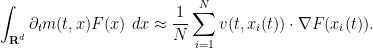
  – smooth, compactly supported functions of space (independent of time). The integral
 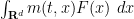 can be viewed as the continuum limit of the sum
  , where
  is the location of the
  agent at time .
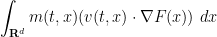
Let us see how this integral should vary in time. At time , the agent should move at velocity  . Differentiating both sides of
using the chain rule, we thus arrive at the heuristic formula
The right-hand side, in the continuum limit , should become
which, after an integration by parts, becomes
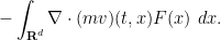
To summarise, for every test function  we have

which leads to the advection equation

Now let us reintroduce the same random noise model that we considered in the previous section. Thus, of all the agents that are infinitesimally close to at time , they will all try to move to  at time
  , but instead each one ends up at a slightly different location
  , where the Brownian path is different for each agent. As such, we are led to the heuristic equation

Taylor expanding the right-hand side as before, and then passing to the continuum limit, we eventually see that the right-hand side takes the form
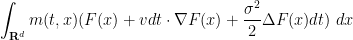
and then repeating the above computations leads us to the Fokker-Planck equation

with  .
.
— 3. Mean field games —
In the derivation of the Hamilton-Jacobi-Bellman equations above, each agent had a fixed cost function to minimise, that did not depend on the location of the other agents. A mean field game generalises this model, by allowing the cost function of each agent to also depend on the density function of all the other agents. For instance, when modeling traffic congestion, the cost function may depend not only on the velocity  that one currently wishes to move at, but also on the density of traffic at that point in space and time.
There are many ways to achieve such a generalisation. The simplest would be an additive model, in which the cost function (1) is replaced with
where  represents the marginal cost to an agent of having a given density at the current location. If is increasing, this intuitively means that the agent prefers to be away from the other agents (a reasonable hypothesis for traffic congestion), which should lead to a repulsive effect; conversely, a decreasing should lead to an attractive effect.
The Hamilton-Jacobi-Bellman equations can be heuristically derived for this cost functional by a similar analysis to before, leading (in the presence of viscosity) to the equation

Meanwhile, the velocity field is still given by the formula (3), so the Fokker-Planck equation (4) becomes (after reversing sign)

The system of (5), (6), with prescribed final data  for at time , and initial data for at time , is then an example of a mean field game. The backward evolution equation (5) represents the agents’ decisions based on where they want to be in the future; and the forward evolution equation (6) represents where they actually end up, based on their initial distribution.
Solving this coupled system of equations, one evolving backwards in time, and one evolving forwards in time, is highly non-trivial, and in some cases existence or uniqueness or both break down (which suggests that the mean field approximation is not valid in this setting). However, there are various situations in which things behave well: having a small (so that the agents only plan ahead for a short period of time), having positive viscosity, and having an increasing (i.e. an aversion to crowds) all help significantly, and one typically has a good existence and uniqueness theory in such cases, based to a large extent on energy methods.
One interesting feature is that when becomes large enough (and in the attractive case when is decreasing), uniqueness can start to break down, due to the existence of standing waves that are sustained solely by nonlinear interactions between the forward evolution equation and the backward one.
The Mexican wave phenomenon can be modeled by a more complicated version of a mean field game. Here, the agents are the audience members of a stadium, and their position is modeled both by a horizontal position (which would be in a bounded two-dimensional domain), as well as an altitude  (they could be sitting, standing, or be in an intermediate position). The agents cannot actually move in the direction, but only in the direction. The cost function consists of three terms: the familiar term that penalises excessive movement, a “comfort” function
  that penalises intermediate positions of between the sitting and standing positions (since it is not comfortable to stay in a half-standing position for any length of time), and the mean field component which penalises those agents at a position whose deviation height
  is too far from the height of nearby agents, in the sense that an integral such as
  , is large. (An audience member who is sitting when everyone is standing, or vice versa, would presumably feel uncomfortable with this status; this is analogous to the attractive case of the potential in the previous example.) It turns out that under reasonable simplifying assumptions, one can create non-trivial travelling wave solutions to this mean field game – but only if the stadium is large enough. The causal mechanism for such waves is somewhat strange, though, due to the presence of the backward propagating equation – in some sense, the wave continues to propagate because the audience members expect it to continue to propagate, and act accordingly. (One wonders if these sorts of equations could provide a model for things like asset price bubbles, which seem to be governed by a similar mechanism.)


45 comments
Comments feed for this article
8 January, 2010 at 7:06 am
Anonymous
Thank you for the post!
I think there is a missing from the
  term in the second-to-last equation in the Hamilton-Jacobi-Bellman equations section (and in the line after that).
[Corrected, thanks – T.]
8 January, 2010 at 9:32 am
Patrick O'Raifearteagh
There is a much simpler way to understand the most recent asset bubble pop without the use of PDEs:draw arrows from the the Wall Street firms to the corporate law firms to the congressman,senators and presidents. Or to put it another way: follow the money.
8 January, 2010 at 9:52 am
Terence Tao
While one can make a case that the decisions of various authorities and influential players exacerbated, or at least failed to mitigate, the effects of the most recent asset price bubble, I think the underlying phenomenon is indeed largely an emergent one arising from the collective behaviour of agents that are not consciously aware of the net consequences of their actions. For instance, similar bubbles have emerged in as mundane a market as that for Beanie Babies, which was unlikely to have been engineered by any government officials, bankers, or even by the toy company itself (which has been unable to replicate the phenomenon ever since, despite strenuous efforts).
Ultimately it would be good to have a theory that combined both the collective behaviour of a large number of “ordinary” agents with the decisions of a few key players of unusually large (relative) influence – some complicated combination of PDE and game theory, presumably – but our current mathematical technology is definitely insufficient for even a zeroth approximation to this task. Until then, I would take any overly simple explanatory theory (e.g. “follow the money”) with a healthy degree of skepticism, though there is undoubtedly a grain of truth to many such explanations.
11 January, 2010 at 10:02 pm
earl thompson
It’s unlikely that modern bubble-creating bureaucrats consciously understand anything like the full magnitude of their anti-social behavior. Yet this new ruling elite has continually adopted startlingly selfish, small-group-optimal, positions at the social cost of a steady disenfranchisement of our middle class. The most recent example of this clubby behavior is the intellectual acceptance of Bernanke’s mid-2008 insistence on stable consumer prices and money supplies in the face of collapsing commodity prices. The trick to predicting such bubbles is to predict the conditions under which the governmental optimum is to empty out the middle class. See my “Predicting Bubbles” paper (#41 on my website), which spends most of its space showing that informationally competitive markets do not produce bubbles.
Beanie babies prices probably did not form a bubble, which require prices to be above fundamental values. Xmas Fashion is uncertain. If a November-produced good becomes a hot product in December, its price will soar. If cold, it’s price will plummet. Ho hum.
Our mathematical technology is just about able us to show that even informational monopolies permit only mini-bubbles, where the monopolist creates an array of minor near-future bubbles in order to prevent future free-riding on his superior future information.
20 January, 2010 at 9:19 pm
Maria
In the case of the asset price bubble, low interest rates and large current account deficit generated excessive liquidity which both motivated and enabled the investment behavior of individual agents. With similar incentives, they behaved similarly and the collective behavior became quite influential. In this particular case, therefore, the collective behavior could be partly described by the incentives behind it, and we can easily put interest rate and CA deficit in a model. I guess describing the incentives rather than the actual behavior of individuals would be more convenient in some other cases as well.
Now, the asset price bubble is still somewhat there, partly due to low interest rates and large government stimulus. The former enabled banks to borrow at very low rates from central banks and use that money to buy high-yielding bonds like long-term Treasuries, and the effect of the later is becoming clear in countries like China where the large stimulus generated inflation. So perhaps some typical behavior of the individual agents could also be captured by setting the level of interest rates, the scale and direction of the stimulus and some other parameters.
14 March, 2017 at 6:16 am
Massimo Fornasier
Not being informed of this particular Terry’s idea, sometimes ago (more or less in 2011) it happened to me to start a research program precisely on what I called “sparse mean-field optimal control”, which is a sort of nonlinear compressed sensing theory, where the nonlinearity is the evolution of a probability distribution and the control is the input to be sparsified to achieve a certain outcome. The possible (many and interesting) applications and implications are clear to grasp. See
Click to access Massimo_Fornasier_proc_7thECM.pdf
8 January, 2010 at 12:17 pm
Anonymous
Hi,
great post. just a small remark: here (section 1) the Legendre transform should be
\displaystyle H(p) := \sup_{v \in {\mathbb R}^d} -v \cdot p – C(v)
and not the usual one from classical mechanics
\displaystyle H(p) := \sup_{v \in {\mathbb R}^d} v \cdot p – C(v)
Rgds,
Diogo Gomes
then the minimal value of {v \cdot \nabla_x u(t_0,x_0) + C(v)} is just {-H(\nabla_x u(t_0,x_0))} (here we use the hypothesis that {C} is even). We conclude that
\displaystyle u(t_0,x_0) = u(t_0,x_0) + dt [ \partial_t u(t_0,x_0) – H(\nabla_x u(t_0,x_0)]
8 January, 2010 at 7:21 pm
Terence Tao
Actually, I think the current sign conventions are consistent (one has to make the substitution and use the hypothesis that C is even).
In Lions’ talk, he reversed time in order to eliminate some of these pesky minus signs, which made the equations slightly nicer but made the connection to the original physical setting less intuitive.
9 January, 2010 at 3:36 am
Anonymous
You’re right – I didn’t see that C was even!
Thanks,
D.
9 January, 2010 at 9:13 am
Jonathan Vos Post
Professor Fellman, Southern New Hampshire University, commented to me by email as follows.
There’s also some strange attractor behavior as well as chaotic transients moving through the system. Think of people trying to get ahead of one another in traffic as a kind of Roshambo game (rock-paper-scissors) with all three different kinds of behavior around the Nash equilibrium depending upon mutation rates. That might help explain why adding more lanes usually creates more rather than less congestion. Also, there’s a problem of dimensionality, since adding more lanes means more orthogonal input which again has “strange” or “chaotic” results on linear or laminar flows. In that sense, I would think that David Ruelle and Floris Takens’ analysis of the transition to turbulence might have some bearing on the problem. There’s something about this buried in Farmer’s 1982 paper on infinite dimensional chaotic attractors as well.
9 January, 2010 at 1:20 pm
PIERRE
“but our current mathematical technology is definitely insufficient for even a zeroth approximation to this task”
Maths have been very useful in physics until now, because mathematics have been created to explain physical phenomenons, such as derivation, variation calculus, differential equation. In physics, you deal with natural phenomenons.
Take the example of planetary systems, meteorology, they are chaotic systems, but the are not impacted by human behaviour. But with economics, you deal with human phenomenons, which are totally different from the physical one.
Exept any recent breakthrough, (e.g games theory), all economic systems have evaded any description. I have seen any profitable application of mathematics in finance.
Put in an other way, is it possible to describe human behaviour with mathematics?
I dont think so.
9 January, 2010 at 5:34 pm
Terence Tao
Well, with our current level of mathematical technology, modeling an individual human is not really feasible, with the important exception of game-theoretic models. But this does not preclude the existence of accurate models that can predict the aggregate behaviour of large populations of human agents. For instance, even though we are unable to predict the behaviour of any given voter in an election a few weeks in the future, we can use electoral polls to obtain predictions as to electoral outcomes that, while not completely accurate, are often superior to any other means of electoral prediction. Large parts of modern advertising and marketing are now based, in part, on statistical models for preferences of human customers which again may not be 100% accurate, but certainly have a non-trivial impact on the effectiveness and utility of such marketing (and companies are willing to invest real sums of money in these sorts of models as a consequence). And mathematical finance has led to a highly liquid market for derivatives which, while obviously prone to rather gross abuse by financial speculators, have also been of significant benefit to the “real” economy. For instance, the wild swings in oil prices in recent years may have wreaked havoc to various speculators, but the sectors which would in the past have been extremely sensitive to such swings – e.g. aviation – have largely protected themselves through hedging, in part due to the ability of mathematical finance to facilitate the transfer of risk to those who are more willing to bear it. (It is true, though, that some financial institutions failed to understand exactly how much risk they were taking on as a consequence; like any other tool, abuses can happen if the underlying mathematical model and its assumptions are not properly understood. It also appears that some fraction of financial activity served not to take risk away from those who were unprepared to accept it, but instead to increase the net risk present in the system; one can hope that future reforms to the financial system can reduce this latter type of activity while preserving the valuable aspects of the former type.)
I believe that in the future, we will have mathematical models that will be better able to accommodate the partly predictable, and partly unknowable, aspects of human behaviour. (In particular, one could hope to develop mathematical tools to try to quantify the robustness of a given system, such as a financial system, to bursts of herd irrationality or other unpredictable group behaviour.) For instance, it is pretty clear that individual human agents in a market do not always behave perfectly rationally; but it is conceivable that if a market is designed in a certain way, that assumptions such as the efficient market hypothesis might still be valid so long as a sufficient proportion of the agents in the market behaved rationally or close to rationally, but that some sort of “phase transition” might occur if a critical mass of irrational agents appeared. I don’t think we currently have the mathematics to precisely discuss these sorts of questions, but in the future we might, and if so I believe these types of questions would be extremely interesting to study.
10 January, 2010 at 1:57 am
Pierre
Thank you for your reply
10 January, 2010 at 4:34 am
Jonathan Vos Post
The late Dr. Isaac Asimov, Professor of Biochemistry at Boston University Medical School, based his “Foundation novels” (originally 3 novels, then integrated with others to make a coherent set of 10 novels, to which there are 3 authorized sequels) on the imaginary future science of “Psychohistory.”
This is a precise Mathematical predictive science of aggregate human behavior. Asimov (who as an undergraduate had trouble deciding between History and Chemistry as a major) hypothesized that for sufficiently large numbers of humans, cooperative effects would occur, and also analogized to the Kinetic Theory of gasses.
I conversed with him about this, as I was only the 2nd active member of Science Fiction Writers of America to have done a doctoral dissertation in Enzymology, and promised him a formal citation to his dissertation in a refereed work, which nobody had done before. Near the end of his prodigiously prolific life (over 500 books) he wrote a story that undercut the assumptions of Psychohistory, explicitly referring to Chaos Theory. The greatest psychohistorian of all time was Hari Seldon.
“I quite understand that psychohistory is a statistical science and cannot predict the future of a single man with any accuracy.”
Among his many books there is also the popularization Asimov On Numbers, Hardcover, 249 pages, Bell Publishing Co. (18 January 1984)
ISBN-10: 0517371456
ISBN-13: 978-0517371459
As the wikipdia entry on him summarizes: Asimov was a long-time member and Vice President of Mensa International, albeit reluctantly; he described some members of that organization as “brain-proud and aggressive about their IQs”, but he also stated that the only two people he had ever met who he would admit were more intelligent than himself were Marvin Minsky and Carl Sagan. He took more joy in being president of the American Humanist Association. The asteroid 5020 Asimov, a crater on the planet Mars, the magazine Asimov’s Science Fiction, a Brooklyn, New York elementary school, and two Isaac Asimov literary awards are named in his honor.
I wrote the biographical article on Isaac Asimov for the Gale Encyclopedia of Computer Science. Isaac Asimov (born Isaac Yudovich Ozimov, Russian: Исаак Юдович Озимов; c. 2 January 1920 – 6 April 1992).
I have an unpublished paper on Asimov Number as an equivalent of Erdos number, linking the biomedical literature’s network of coauthorship with that of Science Fiction.
“Those people who think they know everything are a great annoyance to those of us who do.” — Isaac Asimov.
10 January, 2010 at 8:39 am
Jérôme Chauvet
Hereafter is what I would consider a first achievement in modelling with math collective agents behavior:
Click to access 0912.4760v1.pdf
This wonderful article shows how a 4-dimensional shape space + non lnear form on it has the ability to seize the complex behavior of a moving worm in 3d space. A moving sworm is the collective behavior of thousands of living cells, which relates the refrence above to the subject of this post.
Best wishes
10 January, 2010 at 9:51 am
Patrick O'Raifearteagh
Jonathan Vos Post
It does seem to be the case that adding more traffic lanes does not lead to a decrease in traffic over time . Many Americans understand this from personal experience. I strongly suspect that the rason why this is true is because the US population is now over three hundred million. This would strongly indicate a disequillibrium between US population growth and infrastructure growth. This way of looking at things may give insight into creation and anihilation of economic bubbles.
By it is not a big secret any more as to why the US population continues to grow,grow and grow some more.
Perhaps a crude-or maybe not so crude-approximationtion of the economic bubble problem is to think of the problem in terms of the logistic equation. I don’t really know. I am just tossing it out.
Quite possible growth-growthmania is the economic world view of the dominant economic system in the US-is the problem. It is safe to say that most growth does come to an end.
Professor Tao
Suppose mathematicians and economists are smart enough to mathematically model the economic stuff that now is mathematically inscrutable…then what? A more basic question-to me at least-is the following?:what does mathematically modelling the economy at the fine grain level actually mean? What would be the whole point of doing this?
10 January, 2010 at 10:13 am
Jérôme Chauvet
Our economical system is constantly “feedbacked” by human creativity : everytime one has seized a rule so as to use it for profit, another one brings in novelty in order to disturb the system and make its own profit out of it. Then, having a stable mathematical model for economy would give its discoverer the key to perfect business for a while, then surely generate concurrency, which would make the model incomplete, perhaps obsolete. Can one then envisage an evolving mathematical model, which grow in dimension with time. For economy, the use of endomorphisms is perhaps not convenient for that reason…
10 January, 2010 at 11:51 am
Terence Tao
As for potential applications of modeling (besides their intrinsic mathematical and scientific interest), one important one is that of planning. In Lions’ talks, he mentioned for instance that a good model of traffic congestion could lead to efficient ways to design (and to numerically test) congestion pricing schemes or other incentives in order to achieve as optimal a result as possible. (Note that the goal of traffic management is not always to minimise traffic congestion; in many cases, the goal is instead to maximise traffic capacity or throughput, which is a slightly different objective. Adding more lanes to a freeway is often more successful at the latter type of goal than the former.)
With regard to financial systems, one obvious future application of better mathematical modeling would be to design financial systems that are resistant to emergent effects such as bubbles, as well as to game-theoretic strategies such as collusion or conspiracy, much as modern cryptography allows us to design communication protocols that are resistant to various types of adversarial behaviour. There are already some limited examples of this type of robust system design, for instance in the design of modern spectrum auctions. A related goal is to design a system in such a way that one has some reliable advance warning when some sort of instability is about to occur.
It may well be that there are fundamental “uncertainty principles” that limit the predictability of a system due to the fact that intelligent agents could use such predictability to alter their strategies, but if so it would be good to quantify such uncertainty principles as much as possible, so that one can squeeze as much consistency and stability out of a system as one can (much as the Heisenberg uncertainty principle tells us that one should be shooting for the Shannon-Nyquist rate when processing band-limited signals).
10 January, 2010 at 12:30 pm
Pierre
Can we consider human behaviour as atomic particle movement.
A single human as a total erratic, unexpectable, irrational, behaviour but on a very large scale, we can say that the group as a rational behaviour?
That’s sound easy to tell, harder to put in practice.
10 January, 2010 at 2:01 pm
Patrick O'Raiffearteagh
Pierre, I think Professor Tao is making the case that statistically, psychological irrationality washes out in the aggregate and therfore not significant in understanding macroeconomic processes If this is true, is this unique to statistical equilibrium models? Another question how close is the dictionary between neoclassical economics and statistical mechanics? Is there a partition function analogy?
I think there is something called partial equillibrium models which allow a somewhat significant role of information flows within an economic process. Joseph Stiglitz won a Noble prize for theorizing about the role of information flows in economic processes. I know very little about this stuff.
11 January, 2010 at 2:20 am
Jérôme Chauvet
What sounds risky in planning our economy from a model is the way one could preserve free-will and liberty in it. When we have such a model working in silico, we will be to enforce it into the human society by setting up all constants and variables the way they must be set up for it to work. Due to this, many people will be demanded to do so or so without more choice left, in order to fit with all requirements. If those persons do not earn as much as they wish to with this system (there surely will be some), they will feel like perverting it anyway. And if the only choice left to crack it up is to not cooperate, they will not cooperate, and freeze the machinery; in case there are around 100% agents cooperating in this non-cooperation status quo, one can imagine this could be harmful to the model.
Can whatever model fix this?… In such a model, anything has to be definitely well thought over, even the satisfaction level each agent feels to have in the system!
11 January, 2010 at 10:47 am
Jonathan Vos Post
“What sounds risky in planning our economy from a model is the way one could preserve free-will and liberty in it.” — there was failure of central Planning in the USSR approach has been said be, Mathematically, in terms of the an input-output model, which uses a matrix representation of a nation’s (or a region’s) economy to predict the effect of changes in one industry on others and by consumers, government, and foreign suppliers on the economy. Wassily Leontief (1905-1999) is credited with the development of this analysis. Francois Quesnay developed a cruder version of this technique called Tableau économique. Leontief won the Nobel Memorial Prize in Economic Sciences for his development of this model. The failure of the USSR approach was that, as they did not have (for 5-year plans) the computational ability to invert a 5,000 x 5,000 matrix, they used the economy itself to iteratively do the inversion, and it took more than 5 years to converge to the parameters of a 5-year plan.
Now, we can invert such matrices in silico. But that does not deal with the underlying metaphysics of “free-will and liberty” — as Isaac Asimov explained in narrative.
I’ve been working for over a year on a Model Theory development of Lies and Deception. This is part of a decade-long collaboration with prof. Philip Fellman (Southern New Hampshire University) on a Mathematical Theory of Disinformation. I’ve commented on this in the Blue Eyed Islanders thread. We deeply believe that intelligent agent simulations require axiomatic understanding of the ways in which agents attempt to deceive each other. There is a computational explosion if one naiovely models each agent’s belief set, its belief about each other agent’s belief set, and so to infinity. Hence one uses belief Revision algorithms to prune the tree. I have a hunch that Quantum Computers geat the exponential explosion, but that does not mean that the human brain is a quantum computer. Merely that such models are far from expert consensus. See:
The Definition of Lying and Deception
First published Thu Feb 21, 2008
http://plato.stanford.edu/entries/lying-definition/
Questions central to the philosophical discussion of lying to others and other-deception (or interpersonal deceiving) may be divided into two kinds. Questions of the first kind are definitional. They include the questions of how lying is to be defined, and how deceiving is to be defined, and whether lying is a form of intended deception. Questions of the second kind are moral. They include the questions of whether lying and deceiving are (defeasibly) morally wrong, and whether, if either lying or deception, or both, are defeasibly morally wrong, they are ever morally obligatory, and not just merely morally permissible. In this entry, we only consider questions of the first kind.
* 1. Definition of lying
o 1.1. Statement condition
o 1.2. Untruthfulness condition
o 1.3. Addressee condition
o 1.4. Intention to deceive addressee condition
o 1.5. Objections to the definition of lying
o 1.6. Alternative definitions of lying
* 2. Definition of deception
o 2.1. Objections to the definition of deception
o 2.2. Alternative definition of deception
* Bibliography
* Other Internet Resources
o Cited Resources
* Related Entries
1. Definition of lying
There is no universally accepted definition of lying to others (Kagan 1998, 113)….
11 January, 2010 at 12:19 pm
Jérôme Chauvet
Dear Jonathan,
Your post was really interesting, I mean, over all expectations (I did not know that this kind of study had been done). However, I meant “free-will” and “liberty” not in the metaphysical way, but rather according to the idea that:
– individuals of any system endowed with “free-will” are able to compute by themselves a choice between two or more known options
– individuals granted with “liberty” (or rather “action freedom”) are not hampered externally when performing the action they decided to do.
Regarding the definition of lying, I would say:
– Any system which, with respect to a same piece of information, uses two different versions of it for either keeping it in its own memory or communicating it to another system.
In this definition, if the wrong version is kept internally by the system and the right version is the one provided by it to the environment, then one can say the system is “lying to itself”, but it is not out of range of the definition. It needs perhaps a little more improvement, but it does sound rather universal to me.
Best,
12 January, 2010 at 6:55 am
michael webster
In an stadium which is large enough, there will be a number of attempts to generate the wave. Some will fail, some will work, others meander. It is not clear from the initial size what the outcome will be, and typically there have to be confederates in the stadium for the wave to work.
What does the model say in this regard?
12 January, 2010 at 8:44 am
Terence Tao
This is not well understood at all, from what I gather from Lions’ talk. The mean field game equations describe self-consistent solutions – systems in which the actions of the agents match up with their optimisation computations (so that the agents are indeed correctly optimising their future cost in their current actions). What is not understood well at all right now is how an inconsistent solution (e.g. when some agents want to create a wave, but the wave is not actually appearing) transitions into a consistent one. The situation is more complicated than that of a traditional evolution equation (which only evolves forward in time, and not backward as well), in which one simply sets initial data and solves the relevant Cauchy problem. The causal relationship seems to be much more complicated when one incorporates the agents’ optimisation procedure into the model.
If you like, the mean field games are somewhat analogous to “steady state” solutions (thinking of time as a static variable now, rather than a dynamic one). I presume Pierre and his coauthors must also be thinking about these more general questions, but the mathematics may not yet be in place yet.
5 February, 2010 at 3:47 am
anonymous
Wikipedia seems to imply that the stadium waves go in the opposite direction in Australia. This is a prank, right?
12 January, 2010 at 12:30 pm
Jérôme Chauvet
These steady states could perhaps be seen as strange attractors of some chaotic system.
12 January, 2010 at 1:02 pm
Pierre
“These steady states could perhaps be seen as strange attractors of some chaotic system.”
If you don’t define very clearly what you are talking about, you can see strange attractors, chaotic systems, are this so called “butterfly effect” anywhere you want.
By the way Terence, (you are the one for this question), can we consider the set of prime numbers as a dynamical system,
and has ever been some applications of this field in prime number theory?
Thank you
30 March, 2010 at 6:41 pm
Mean field games « Andrea Bedini
[…] Mean field games Link: Mean field games […]
9 April, 2010 at 3:59 pm
Swarms, Crowds, and PDE’s « Big Numbers
[…] a link to an earlier talk of Lions’ on mean field games at UCLA. Terence Tao has a lovely and more detailed exposition on his […]
10 December, 2010 at 7:11 am
LOG | WHAT I BELIEVE
[…] Mean field games seem to be potential tools for the project. This entry was posted in Log. Bookmark the permalink. […]
7 February, 2011 at 2:24 pm
mean_field_games [Adam Tilton's Wiki]
[…] https://terrytao.wordpress.com/2010/01/07/mean-field-equations/ […]
11 April, 2011 at 10:24 am
Anonymous
Hello,
Apologies if this is an embarrassing mistake. But isn’t there a missing $\nabla_x$ in the definition of $p$ after the equation $\tilde v \cdot p – C(\tilde v)$?
[Corrected, thanks – T.]
17 November, 2013 at 10:01 pm
Les jeux à champ moyen | 2013, année des Mathématiques de la Planète Terre
[…] long post du blog de T. Tao sur les jeux à champ moyen [En […]
12 January, 2014 at 8:19 am
Riccardo
Thank you Professor for this post. It was very interesting and very well explained.
11 March, 2014 at 12:47 am
nikhil
Prof. Tao, this is a very nice expository article for an engineering student like me who is interested in doing more mathematical stuff……what is a good expository book on mean field games
Thanks
Nikhil
11 March, 2014 at 1:12 am
2pg
Hey.
Is the mean field games theory used in optimization techniques that involve flow?
Very interesting read for an engineering major
5 December, 2014 at 1:53 pm
Leonid
Qualitatively, leaving aside the exact mathematical details, this is nothing conceptually new for economists — the structure described here is what is known as rational expectations economics. Agents make plans today based on their understanding (assumed to be perfect) of the future evolution of the aggregate economy, which itself depends on the individual choices.
There is a relation to bubbles, that’s correct. That’s just a special topic in the broader area (above), known as rational bubbles.
As for the interaction of the irrational and rational agents, this can be analyzed using conventional methods. There is a literature on market selection that deals with this exact question: how does the presence of irrational agents affect the aggregate market dynamics.
8 June, 2016 at 10:53 am
zhengli0817
Reblogged this on dataquantblog and commented:
A nice and intuitive introduction to mean field games
14 October, 2016 at 2:04 am
Vincent Leclere
Thanks for this presentation. I remarked that the link to the Lion’s series of lecture is dead. Here is a working link on the subject :
MFG and application https://www.college-de-france.fr/site/pierre-louis-lions/course-2010-11-12-09h00.htm
11 November, 2016 at 2:25 pm
Olivier Wang
The key challenge one faces when trying to model bubbles is to embed intuitions like the self-fulfilling force you mention into familiar models of financial markets based on the principle of no-arbitrage. Often, this principle is too strong for the initial intuition to survive: to take your example, the modeler must defend why wealthy, risk-neutral traders who are less affected by the discomfort u(z) would not take advantage of the crowd of traders sensitive to u(z) by short-selling the asset, which eventually prevents the price bubble to form or grow. While each of the conditions implicit in my previous sentence could be relaxed in turn (for instance by arguing that these rational traders would need an enormous amount of wealth to be able to move the market, or that it would expose them to too much risk in the short-run, like LTCM https://en.wikipedia.org/wiki/Long-Term_Capital_Management), here is an interesting example by Dilip Abreu and Markus Brunnermeier that relies on a concept you wrote about recently, common knowledge (or lack thereof): https://www.princeton.edu/~markus/research/papers/bubbles_crashes.pdf
The idea is that even if these ‘rational’ traders exist and are well-informed enough to know that the asset is overvalued, it could be much harder for them to know whether other market participants also know that other market participants also know that … also know that the asset is overvalued.
27 March, 2017 at 5:43 am
kenneth
Some minor typos are spotted in the post. [a] In the third equation from the last of the first section on HJB, may be missing from the term
  ; [b] There seems one more closing parenthesis included in the equation (6); [c] In the equation right before the equation (4),
  may be missing right after the term
  ; [d] In the equation (4), the viscosity
  may be better to be replaced by
  , since
  is just mentioned once way earlier in the first section.
[Corrected, thanks – T.]
9 August, 2017 at 12:09 pm
Krishna Bhogaonker
Hello Prof. Tao. This discussion on mean field games is fascinating. I was wondering if you have any more writings on the mathematics of human behavior, etc?
The reason I ask is because the viewpoint here does differ quite substantially from the classical political science or sociological approaches to human behavior analysis. For example, you mention two potential applications of human behavior modelling–planning and testing the robustness of systems (eg. financial). I think one strand of political/sociological thought (Frankfurt school) would suggest the dangers of this form of analysis as it could be used by the more powerful interests in society to enforce control over the 99% of the population. For example using behavior models to generate fake news that elects specific candidates who undermine healthcare for the people who elected them.
Of course there it truth on both sides of the argument. Modeling can have very positive effects to help improve the welfare of individuals, as well as very negative effects. So I think the real question is how to use modelling to create boundaries or guardrails that prevent these technologies being used for nefarious purposes–as best as possible.
If you have any additional views or writings on modelling behavior, could you please provide links. I know that you are terribly busy, so if you don’t have a chance to then I understand.
16 August, 2021 at 8:23 pm
sumit
how can i do mean field game compute simulation?
any resource link would be much appreciated.
13 November, 2021 at 2:05 pm
Just curious
Can the techniques be helpful in crowd management just as it helps predict Mexican wave? https://www.msn.com/en-us/sports/ncaabk/ucla-students-describe-terrifying-scene-amid-crush-of-bodies-outside-pauley-pavilion/ar-AAQEMy1