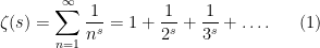
The Riemann zeta function  is defined in the region
  by the absolutely convergent series
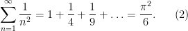
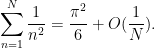
Thus, for instance, it is known that  , and thus
For  , the series on the right-hand side of (1) is no longer absolutely convergent, or even conditionally convergent. Nevertheless, the
  function can be extended to this region (with a pole at
  ) by analytic continuation. For instance, it can be shown that after analytic continuation, one has
  ,
,  , and
, and  , and more generally
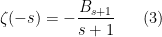
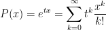
for  , where
  are the Bernoulli numbers. If one formally applies (1) at these values of
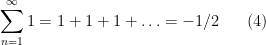
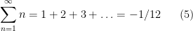
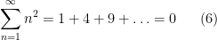
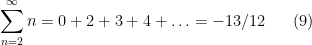
  , one obtains the somewhat bizarre formulae
and

Clearly, these formulae do not make sense if one stays within the traditional way to evaluate infinite series, and so it seems that one is forced to use the somewhat unintuitive analytic continuation interpretation of such sums to make these formulae rigorous. But as it stands, the formulae look “wrong” for several reasons. Most obviously, the summands on the left are all positive, but the right-hand sides can be zero or negative. A little more subtly, the identities do not appear to be consistent with each other. For instance, if one adds (4) to (5), one obtains
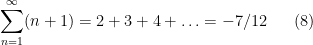
whereas if one subtracts  from (5) one obtains instead
and the two equations seem inconsistent with each other.
However, it is possible to interpret (4), (5), (6) by purely real-variable methods, without recourse to complex analysis methods such as analytic continuation, thus giving an “elementary” interpretation of these sums that only requires undergraduate calculus; we will later also explain how this interpretation deals with the apparent inconsistencies pointed out above.
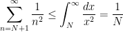
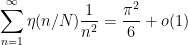
To see this, let us first consider a convergent sum such as (2). The classical interpretation of this formula is the assertion that the partial sums
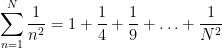
converge to  as
as  , or in other words that
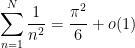
where  denotes a quantity that goes to zero as . Actually, by using the integral test estimate
we have the sharper result
Thus we can view  as the leading coefficient of the asymptotic expansion of the partial sums of
  .
.
One can then try to inspect the partial sums of the expressions in (4), (5), (6), but the coefficients bear no obvious relationship to the right-hand sides:

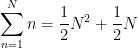

For (7), the classical Faulhaber formula (or Bernoulli formula) gives
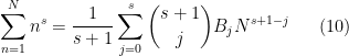
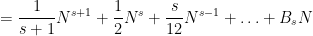
for  , which has a vague resemblance to (7), but again the connection is not particularly clear.
The problem here is the discrete nature of the partial sum

which (if  is viewed as a real number) has jump discontinuities at each positive integer value of . These discontinuities yield various artefacts when trying to approximate this sum by a polynomial in . (These artefacts also occur in (2), but happen in that case to be obscured in the error term
  ; but for the divergent sums (4), (5), (6), (7), they are large enough to cause real trouble.)
However, these issues can be resolved by replacing the abruptly truncated partial sums  with smoothed sums
  , where
  is a cutoff function, or more precisely a compactly supported bounded function that is right-continuous the origin and equals at
  . The case when
  is the indicator function
 ![{1_{[0,1]}}](https://s0.wp.com/latex.php?latex=%7B1_%7B%5B0%2C1%5D%7D%7D&bg=ffffff&fg=000000&s=0&c=20201002) then corresponds to the traditional partial sums, with all the attendant discretisation artefacts; but if one chooses a smoother cutoff, then these artefacts begin to disappear (or at least become lower order), and the true asymptotic expansion becomes more manifest.
then corresponds to the traditional partial sums, with all the attendant discretisation artefacts; but if one chooses a smoother cutoff, then these artefacts begin to disappear (or at least become lower order), and the true asymptotic expansion becomes more manifest.
Note that smoothing does not affect the asymptotic value of sums that were already absolutely convergent, thanks to the dominated convergence theorem. For instance, we have
whenever is a cutoff function (since  pointwise as and is uniformly bounded). If is equal to on a neighbourhood of the origin, then the integral test argument then recovers the decay rate:
However, smoothing can greatly improve the convergence properties of a divergent sum. The simplest example is Grandi’s series
The partial sums
oscillate between and , and so this series is not conditionally convergent (and certainly not absolutely convergent). However, if one performs analytic continuation on the series
and sets  , one obtains a formal value of
  for this series. This value can also be obtained by smooth summation. Indeed, for any cutoff function , we can regroup

If is twice continuously differentiable (i.e.  ), then from Taylor expansion we see that the summand has size
  , and also (from the compact support of ) is only non-zero when
  . This leads to the asymptotic
and so we recover the value of as the leading term of the asymptotic expansion.
Exercise 1 Show that if is merely once continuously differentiable (i.e.  ), then we have a similar asymptotic, but with an error term of instead of . This is an instance of a more general principle that smoother cutoffs lead to better error terms, though the improvement sometimes stops after some degree of regularity.
Remark 2 The most famous instance of smoothed summation is Cesáro summation, which corresponds to the cutoff function  . Unsurprisingly, when Cesáro summation is applied to Grandi’s series, one again recovers the value of .
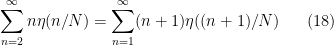
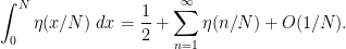
If we now revisit the divergent series (4), (5), (6), (7) with smooth summation in mind, we finally begin to see the origin of the right-hand sides. Indeed, for any fixed smooth cutoff function , we will shortly show that
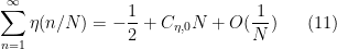
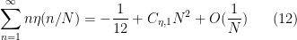

and more generally

for any fixed  where
where  is the Archimedean factor
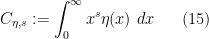
(which is also essentially the Mellin transform of ). Thus we see that the values (4), (5), (6), (7) obtained by analytic continuation are nothing more than the constant terms of the asymptotic expansion of the smoothed partial sums. This is not a coincidence; we will explain the equivalence of these two interpretations of such sums (in the model case when the analytic continuation has only finitely many poles and does not grow too fast at infinity) below the fold.
This interpretation clears up the apparent inconsistencies alluded to earlier. For instance, the sum  consists only of non-negative terms, as does its smoothed partial sums
 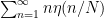 (if is non-negative). Comparing this with (12), we see that this forces the highest-order term
  to be non-negative (as indeed it is), but does not prohibit the lower-order constant term
  from being negative (which of course it is).
Similarly, if we add together (12) and (11) we obtain

while if we subtract from (12) we obtain

These two asymptotics are not inconsistent with each other; indeed, if we shift the index of summation in (17), we can write
and so we now see that the discrepancy between the two sums in (8), (9) come from the shifting of the cutoff  , which is invisible in the formal expressions in (8), (9) but become manifestly present in the smoothed sum formulation.
Exercise 3 By Taylor expanding  and using (11), (18) show that (16) and (17) are indeed consistent with each other, and in particular one can deduce the latter from the former.
— 1. Smoothed asymptotics —
We now prove (11), (12), (13), (14). We will prove the first few asymptotics by ad hoc methods, but then switch to the systematic method of the Euler-Maclaurin formula to establish the general case.
For sake of argument we shall assume that the smooth cutoff is supported in the interval ![{[0,1]}](https://s0.wp.com/latex.php?latex=%7B%5B0%2C1%5D%7D&bg=ffffff&fg=000000&s=0&c=20201002) (the general case is similar, and can also be deduced from this case by redefining the parameter). Thus the sum
(the general case is similar, and can also be deduced from this case by redefining the parameter). Thus the sum  is now only non-trivial in the range
  .
.
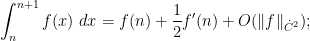
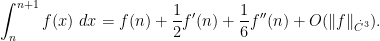
To establish (11), we shall exploit the trapezoidal rule. For any smooth function  , and on an interval
 ![{[n,n+1]}](https://s0.wp.com/latex.php?latex=%7B%5Bn%2Cn%2B1%5D%7D&bg=ffffff&fg=000000&s=0&c=20201002) , we see from Taylor expansion that
, we see from Taylor expansion that

for any  ,
,  . In particular we have

and
eliminating  , we conclude that

Summing in  , we conclude the trapezoidal rule

We apply this with  , which has a
  norm of from the chain rule, and conclude that
But from (15) and a change of variables, the left-hand side is just  . This gives (11).
The same argument does not quite work with (12); one would like to now set  , but the norm is now too large ( instead of ). To get around this we have to refine the trapezoidal rule by performing the more precise Taylor expansion

where  . Now we have

and
We cannot simultaneously eliminate both and  . However, using the additional Taylor expansion

one obtains

and thus on summing in , and assuming that  vanishes to second order at , one has (by telescoping series)

We apply this with . After a few applications of the chain rule and product rule, we see that  ; also,
  ,
,  , and
, and  . This gives (12).
The proof of (13) is similar. With a fourth order Taylor expansion, the above arguments give


and

Here we have a minor miracle (equivalent to the vanishing of the third Bernoulli number  ) that the
  term is automatically eliminated when we eliminate the
  term, yielding


and thus

With  , the left-hand side is
  , the first two terms on the right-hand side vanish, and the
  norm is , giving (13).
Now we do the general case (14). We define the Bernoulli numbers  recursively by the formula

for all  , or equivalently

The first few values of  can then be computed:

From (19) we see that
![\displaystyle \sum_{k=0}^\infty \frac{B_k}{k!} [ P^{(k)}(1) - P^{(k)}(0) ] = P'(1) \ \ \ \ \ (20)](https://s0.wp.com/latex.php?latex=%5Cdisplaystyle+%5Csum_%7Bk%3D0%7D%5E%5Cinfty+%5Cfrac%7BB_k%7D%7Bk%21%7D+%5B+P%5E%7B%28k%29%7D%281%29+-+P%5E%7B%28k%29%7D%280%29+%5D+%3D+P%27%281%29+%5C+%5C+%5C+%5C+%5C+%2820%29&bg=ffffff&fg=000000&s=0&c=20201002)
for any polynomial  (with
(with  being the
  -fold derivative of ); indeed, (19) is precisely this identity with
  , and the general case then follows by linearity.
As (20) holds for all polynomials, it also holds for all formal power series (if we ignore convergence issues). If we then replace by the formal power series
we conclude the formal power series (in  ) identity
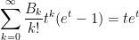
leading to the familiar generating function
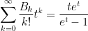
for the Bernoulli numbers.
If we apply (20) with equal to the antiderivative of another polynomial  , we conclude that
![\displaystyle \int_0^1 Q(x)\ dx + \frac{1}{2} (Q(1)-Q(0)) + \sum_{k=2}^\infty \frac{B_k}{k!} [Q^{(k-1)}(1) - Q^{(k-1)}(0)] = Q(1)](https://s0.wp.com/latex.php?latex=%5Cdisplaystyle+%5Cint_0%5E1+Q%28x%29%5C+dx+%2B+%5Cfrac%7B1%7D%7B2%7D+%28Q%281%29-Q%280%29%29+%2B+%5Csum_%7Bk%3D2%7D%5E%5Cinfty+%5Cfrac%7BB_k%7D%7Bk%21%7D+%5BQ%5E%7B%28k-1%29%7D%281%29+-+Q%5E%7B%28k-1%29%7D%280%29%5D+%3D+Q%281%29&bg=ffffff&fg=000000&s=0&c=20201002)
which we rearrange as the identity
![\displaystyle \int_0^1 Q(x)\ dx = \frac{1}{2}(Q(0)+Q(1)) - \sum_{k=2}^\infty \frac{B_k}{k!} [Q^{(k-1)}(1) - Q^{(k-1)}(0)]](https://s0.wp.com/latex.php?latex=%5Cdisplaystyle+%5Cint_0%5E1+Q%28x%29%5C+dx+%3D+%5Cfrac%7B1%7D%7B2%7D%28Q%280%29%2BQ%281%29%29+-+%5Csum_%7Bk%3D2%7D%5E%5Cinfty+%5Cfrac%7BB_k%7D%7Bk%21%7D+%5BQ%5E%7B%28k-1%29%7D%281%29+-+Q%5E%7B%28k-1%29%7D%280%29%5D&bg=ffffff&fg=000000&s=0&c=20201002)
which can be viewed as a precise version of the trapezoidal rule in the polynomial case. Note that if has degree  , the only the summands with
  can be non-vanishing.
Now let be a smooth function. We have a Taylor expansion

for  and some polynomial of degree at most
  ; also

for and  . We conclude that

![\displaystyle - \sum_{k=2}^{s+1} \frac{B_k}{k!} [f^{(k-1)}(1) - f^{(k-1)}(0)]](https://s0.wp.com/latex.php?latex=%5Cdisplaystyle+-+%5Csum_%7Bk%3D2%7D%5E%7Bs%2B1%7D+%5Cfrac%7BB_k%7D%7Bk%21%7D+%5Bf%5E%7B%28k-1%29%7D%281%29+-+f%5E%7B%28k-1%29%7D%280%29%5D&bg=ffffff&fg=000000&s=0&c=20201002)

Translating this by an arbitrary integer (which does not affect the  norm), we obtain
![\displaystyle - \sum_{k=2}^{s+1} \frac{B_k}{k!} [f^{(k-1)}(n+1) - f^{(k-1)}(n)] + O( \|f\|_{\dot C^{s+2}} ).](https://s0.wp.com/latex.php?latex=%5Cdisplaystyle+-+%5Csum_%7Bk%3D2%7D%5E%7Bs%2B1%7D+%5Cfrac%7BB_k%7D%7Bk%21%7D+%5Bf%5E%7B%28k-1%29%7D%28n%2B1%29+-+f%5E%7B%28k-1%29%7D%28n%29%5D+%2B+O%28+%5C%7Cf%5C%7C_%7B%5Cdot+C%5E%7Bs%2B2%7D%7D+%29.+&bg=ffffff&fg=000000&s=0&c=20201002)
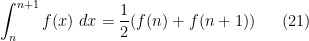
Summing the telescoping series, and assuming that vanishes to a sufficiently high order at , we conclude the Euler-Maclaurin formula


We apply this with  . The left-hand side is
  . All the terms in the sum vanish except for the
  term, which is
  . Finally, from many applications of the product rule and chain rule (or by viewing
  where
where  is the smooth function
  ) we see that
  , and the claim (14) follows.
Remark 4 By using a higher regularity norm than the norm, we see that the error term can in fact be improved to  for any fixed
  , if is sufficiently smooth.
Exercise 5 Use (21) to derive Faulhaber’s formula (10). Note how the presence of boundary terms at cause the right-hand side of (10) to be quite different from the right-hand side of (14); thus we see how non-smooth partial summation creates artefacts that can completely obscure the smoothed asymptotics.
— 2. Connection with analytic continuation —
Now we connect the interpretation of divergent series as the constant term of smoothed partial sum asymptotics, with the more traditional interpretation via analytic continuation. For sake of concreteness we shall just discuss the situation with the Riemann zeta function series  , though the connection extends to far more general series than just this one.
In the previous section, we have computed asymptotics for the partial sums

when is a negative integer. A key point (which was somewhat glossed over in the above analysis) was that the function  was smooth, even at the origin; this was implicitly used to bound various
  norms in the error terms.
Now suppose that is a complex number with  , which is not necessarily a negative integer. Then becomes singular at the origin, and the above asymptotic analysis is not directly applicable. However, if one instead considers the telescoped partial sum
with equal to near the origin, then by applying (22) to the function  (which vanishes near the origin, and is now smooth everywhere), we soon obtain the asymptotic


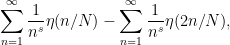
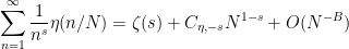
Applying this with equal to a power of two and summing the telescoping series, one concludes that
for some complex number which is basically the sum of the various terms appearing in (23). By modifying the above arguments, it is not difficult to extend this asymptotic to other numbers than powers of two, and to show that is independent of the choice of cutoff .
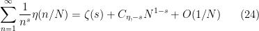
From (24) we have
which can be viewed as a definition of in the region . For instance, from (14), we have now proven (3) with this definition of . However it is difficult to compute exactly for most other values of .
For each fixed , it is not hard to see that the expression  is complex analytic in . Also, by a closer inspection of the error terms in the Euler-Maclaurin formula analysis, it is not difficult to show that for in any compact region of
  , these expressions converge uniformly as . Applying Morera’s theorem, we conclude that our definition of is complex analytic in the region
  .
.
We still have to connect this definition with the traditional definition (1) of the zeta function on the other half of the complex plane. To do this, we observe that

for large enough. Thus we have
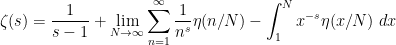
for  . The point of doing this is that this definition also makes sense in the region
  (due to the absolute convergence of the sum and integral
  . By using the trapezoidal rule, one also sees that this definition makes sense in the region
  , with locally uniform convergence there also. So we in fact have a globally complex analytic definition of
  , and thus a meromorphic definition of on the complex plane. Note also that this definition gives the asymptotic

near , where  is Euler’s constant.
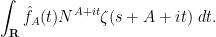
We have thus seen that asymptotics on smoothed partial sums of  gives rise to the familiar meromorphic properties of the Riemann zeta function . It turns out that by combining the tools of Fourier analysis and complex analysis, one can reverse this procedure and deduce the asymptotics of from the meromorphic properties of the zeta function.
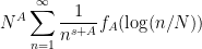
Let’s see how. Fix a complex number with  , and a smooth cutoff function which equals one near the origin, and consider the expression
where is a large number. We let  be a large number, and rewrite this as
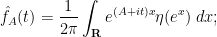
where

The function  is in the Schwartz class. By the Fourier inversion formula, it has a Fourier representation
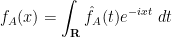
where

and so (26) can be rewritten as
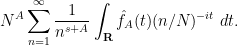
The function  is also Schwartz. If
  is large enough, we may then interchange the integral and sum and use (1) to rewrite (26) as
Now we have
integrating by parts (which is justified when is large enough) we have

where

We can thus write (26) as a contour integral
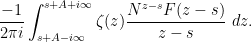
Note that  is compactly supported away from zero, which makes
  an entire function of
  , which is uniformly bounded whenever is bounded. Furthermore, from repeated integration by parts we see that is rapidly decreasing as
  , uniformly for in a compact set. Meanwhile, standard estimates show that
  is of polynomial growth in for
  in a compact set. Finally, the meromorphic function
  has a simple pole at
  (with residue
  ) and at
  (with residue
  ). Applying the residue theorem, we can write (26) as

for any . Using the various bounds on and  , we see that the integral is
  . From integration by parts we have
  and
and

and thus we have
for any , which is (14) (with the refined error term indicated in Remark 4).
The above argument reveals that the simple pole of at is directly connected to the  term in the asymptotics of the smoothed partial sums. More generally, if a Dirichlet series
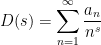
has a meromorphic continuation to the entire complex plane, and does not grow too fast at infinity, then one (heuristically at least) has the asymptotic
where  ranges over the poles of
  , and
, and  are the residues at those poles. For instance, one has the famous explicit formula

where  is the von Mangoldt function, are the non-trivial zeroes of the Riemann zeta function (counting multiplicity, if any), and
  is an error term (basically arising from the trivial zeroes of zeta); this ultimately reflects the fact that the Dirichlet series

has a simple pole at (with residue  ) and simple poles at every zero of the zeta function with residue
  (weighted again by multiplicity, though it is not believed that multiple zeroes actually exist).
The link between poles of the zeta function (and its relatives) and asymptotics of (smoothed) partial sums of arithmetical functions can be used to compare elementary methods in analytic number theory with complex methods. Roughly speaking, elementary methods are based on leading term asymptotics of partial sums of arithmetical functions, and are mostly based on exploiting the simple pole of at (and the lack of a simple zero of Dirichlet  -functions at ); in contrast, complex methods also take full advantage of the zeroes of and Dirichlet -functions (or the lack thereof) in the entire complex plane, as well as the functional equation (which, in terms of smoothed partial sums, manifests itself through the Poisson summation formula). Indeed, using the above correspondences it is not hard to see that the prime number theorem (for instance) is equivalent to the lack of zeroes of the Riemann zeta function on the line
  .
.
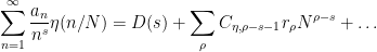
With this dictionary between elementary methods and complex methods, the Dirichlet hyperbola method in elementary analytic number theory corresponds to analysing the behaviour of poles and residues when multiplying together two Dirichlet series. For instance, by using the formula (11) and the hyperbola method, together with the asymptotic

which can be obtained from the trapezoidal rule and the definition of , one can obtain the asymptotic
where  is the divisor function (and in fact one can improve the
  bound substantially by being more careful); this corresponds to the fact that the Dirichlet series

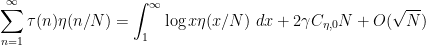
has a double pole at with expansion
and no other poles, which of course follows by multiplying (25) with itself.
Remark 6 In the literature, elementary methods in analytic number theorem often use sharply truncated sums rather than smoothed sums. However, as indicated earlier, the error terms tend to be slightly better when working with smoothed sums (although not much gain is obtained in this manner when dealing with sums of functions that are sensitive to the primes, such as , as the terms arising from the zeroes of the zeta function tend to dominate any saving in this regard).


218 comments
Comments feed for this article
27 January, 2017 at 12:08 pm
¿Qué sorpresas esconden las sumas infinitas? I | Una vista circular
[…] 1 + 2 + 3 + 4 + ….. Yo he aprendido este enfoque, que quizás no es aún muy conocido, en un magnífico post en el blog de Terence Tao. Mi objetivo en esta serie de posts es dar los detalles imprescindibles […]
30 January, 2017 at 9:25 pm
kolmogorovscale
Reblogged this on Stat Phys Bio Chem.
25 June, 2017 at 3:51 pm
Why -1/12? – Maths and Machine Learning
[…] very thorough (and reasonably accessible) discussion of the above series can be found in Terrence Tao’s blog post. In this post, I will not be attempting to either match the rigor or the comprehensiveness of […]
22 July, 2017 at 7:03 am
Dr. Enoch Opeyemi
Greetings Prof. Tao,
Over the years,I have been working on the Riemann Hypothesis and I have recently found some results that might be interesting to you sir.
I would like your comments and contributions on them because I got to a point at which I need to use analytic continuation method on my finding.
Thank you Sir!
6 September, 2017 at 6:04 am
Zeta function regularization – Amplitudes. . .
[…] you can read about divergent series in the following post by Terence Tao and in the book Divergent Series by Hardy. The Riemann hypothesis is an open problem in math, and […]
9 September, 2017 at 2:00 am
Jose Javier Garcia Moreta
Dear professor tao.. for the case of the general harmonic series
\sum_{n=0}^{\infty} \frac{1}{(n+a)}? is this \-Psi(a) or \|-\Psi (a)+log(a) ??
which one is the correct regularized result ??
17 September, 2017 at 11:52 am
Bernard Montaron
Here is another strange equality, which might be compared to equation (7):


And here is the proof of this: Clearly 10S = S – 1 (!)
And since 1/9 = 0.111111… this leads to
You can generalize this to any rational number, like e.g.
And with 1/7 = 0.142857142857… it follows that
Sorry about this!
1 November, 2017 at 9:13 am
B. Koller
A question of terminology :
I have a rather naive question. We can prove in a strictly mathematical sense that the sum over all the natural numbers must be positive, for instance by induction. If on the other side we put the sum of all natural numbers equal to -1/12 then we prove the contradiction -1/12 > 0 and one knows that from a contradiction everything follows.
So should we not write instead of the equal sign =, which stands for an equivalence relation and is therefore transitive, the sign : from logic which is in my understanding not an equivalence relation and is not giving a contradiction. I know this is not done usually in mathematics, but it would have the advantage to create less misunderstandings.
Thanks
PS. Prof. Tao approach gave me a much better understanding of infinite series, thanks a lot.
21 November, 2017 at 8:42 pm
Ángel Méndez Rivera
“We can prove in a strictly mathematical sense that the sum over all the natural numbers must be positive, for instance by induction.”
This is not true. You can only prove by induction that the sum of finitely many addends, all of which are elements of set of natural numbers, must itself be a natural number. However, this proof cannot be executed with infinitely many addends, since it can be rigorously proven that infinite sums are in general not commutative, nor are they closed under any subset of the real numbers, nor are they associative.
“If on the other side we put the sum of all natural numbers equal to -1/12 then we prove the contradiction -1/12 > 0”
You’re assuming the sum is greater than zero, which is not. Terence Tao provided an explanation of why this is the case. Whenever N is finite, the term of the highest order in asymptotic expansion, C(η,1)N^2, is always positive and larger in magnitude than 1/12. However, this can be shown false whenever N is infinite.
“So should we not write instead of the equal sign =, which stands for an equivalence relation and is therefore transitive, the sign : from logic which is in my understanding not an equivalence relation and is not giving a contradiction.”
There is no contradiction. Mathematicians have been using = for centuries, and the reason is that the usage of it is not wrong.
“I know this is not done usually in mathematics, but it would have the advantage to create less misunderstandings.”
There is no misunderstanding. The = is meant literally here, because there are methods to prove that both expressions in the equation are EQUAL, they do not merely correspond to each other, but are actually equivalent.
15 July, 2023 at 1:38 pm
Wolfgang Mückenheim
Adding positive values finitely or infinitely often will never result in a decrease.
8 October, 2018 at 2:21 am
Ángel Méndez Rivera
Also, to add to my response to the comment, your claim that everything follows from a contradiction is not true. The principle of explosion is merely an axiom of classical propositional logic, but arithmetic first-order logic uses a Hilbert-style deduction system, in which the principle of explosion cannot be proven nor disproven.
30 November, 2017 at 3:17 pm
1+2+3+4+ … = –1/12 | Maths with a Pinch of Salt
[…] Terence Tao (o różnych sposobach „sumowania” nieskończonych sum) […]
14 December, 2017 at 1:26 pm
1+2+3+4+ … = –1/12 – Mathematica cum grano salis
[…] Terence Tao (on the many ways of making sense of „impossible” sums) […]
3 March, 2018 at 5:27 am
Aditya Ghosh
Reblogged this on Mathematics Support.
3 May, 2018 at 1:44 am
Clément Caubel
Just to mention a little mistake/typo: after the proof of the Euler-MacLaurin formula (22), when deducing the claim (14), the left hand side is (and not
  ). Also, the size
  is used during the introduction, and then replaced by
  .
.
This gives me the opportunity to thank you warmly for sharing your notes on this blog!
[Corrected, thanks -T.]
7 July, 2018 at 1:32 pm
Is String Theory Built On Funny Math? | Physics Forums
[…] if you want more heavy math see the blog by Terry Tao the guy that started me thinking about this: https://terrytao.wordpress.com/2010…tion-and-real-variable-analytic-continuation/ Now the 64 million dollar question is this, Look in video 1 – he opens a string theory text – low […]
1 August, 2018 at 8:00 am
The Sum Of All Numbers Is -1/12? – This Week I Found Out
[…] https://terrytao.wordpress.com/2010/04/10/the-euler-maclaurin-formula-bernoulli-numbers-the-zeta-fun… […]
5 August, 2018 at 9:41 am
Fake papers #1: L’uomo che scambiò la Zeta di Riemann per un polinomio | Maddmaths!
[…] Per farsi un’idea di come questa procedura sia di difficile comprensione per i non esperti, usando la continuazione analitica si arriva a scrivere [1+2+3+4+dots “=” -frac{1}{12}] dove i puntini a sinistra dell’uguale indicano che vanno sommati tutti i numeri naturali, mentre l’uguale è scritto tra virgolette proprio ad indicare che non si tratta di una vera uguaglianza, ma di un’uguaglianza che ha senso usando la procedura di continuazione analitica. Non ha infatti molto senso pensare che la somma di tutti i numeri naturali, infiniti e tutti positivi, sia uguale a un numero razionale e per di più negativo! In effetti la formula nasce dalla continuazione analitica proprio della funzione zeta di Riemann, e ci dice che (-frac{1}{12}) è il valore della funzione (zeta(s)) per (s=-1). Se volete saperne di più su somme di questo tipo, senza usare la continuazione analitica, potete consultare l’articolo tecnico sul blog di Terence Tao. […]
7 October, 2018 at 4:14 pm
Jotvansh
Hi, Professor Tao
I am a highschool student, I was really fascinated with with this theorem as it contradicts the basic principles of mathematics, so I chose this my mathematical reasacrch project, however I have to prove this summation in an less rigorous way. I have used Grandi series and Ceasaro convergent in order to use for this equation. Although, I am not really sure it would be correct to use them to manipulate the series.
8 October, 2018 at 2:09 am
Ángel Méndez Rivera
First of all, you are wrong. The theorem does not contradict the basic principles of mathematics. In fact, I question whether you can even correctly list all the basic principles of mathematics you are appealing to. My guess is that you cannot. This is not surprising, since such principles are typically never taught until you have reached a graduate level of mathematical education. In any case, the very fact that it is a theorem implies it cannot be in contradiction with the principles, because by definition, theorems are derivable only from principles. If you conclude that mathematical claim contradicts the principles, then either the claim is not a theorem, or else your understanding of the principles is incorrect.
Second of all, Cèsaro summations are not useable for this series, because this series is outside the domain of the Cèsaro summations. The Grandi series is not linearly nor polynomially related to the Ramanujan series. You must use some other method to prove the theorem.
16 July, 2023 at 5:37 am
Wolfgang Mckenhei8m
A theorem can imply a contradiction if the basics are inconsistent. Here: Only geometric series with q less than 1 can be summed in a meaningful way. Further summing infinit sets obeys the same logic as summing finite sets: Adding only positive values cannot reduce the result. Finally we need not look for the reasons if the result is blatantly false like -1/12 > 1.
29 January, 2019 at 4:00 pm
Jerome
@RIvera I support your patience.
A small linguistic remark. In the context of these ‘provocative’ limits (they are not a provocation at all to me.).
I might be good avoid saying ‘this series has such limit’ and say this series is given such limit.
In fact what matters before all is that the limit we GIVE commute with finite sums.
29 July, 2019 at 4:17 am
Karl Svozil
May formula (12) not also be interpreted as a consequence or rather an instance of Ritt’s theorem? And therefore (14) a generalization thereof?
(Please excuse this naive question of a humble physicist; and thank you for this very nice post!)
30 August, 2019 at 11:26 pm
Terence Tao - Understanding 1+2+3+...=-1/12 without Complex Analysis - Nevin Manimala's Blog
[…] by /u/MysteriousSeaPeoples [link] […]
29 September, 2019 at 4:44 am
Michele Nardelli
Dear Prof. Tao,
I deal mainly of the new possible mathematical connections, between various formulas of some sectors of theoretical physics and some formulas of specific areas of Number Theory, especially the mathematics of the Indian genius S. Ramanujan (Rogers-Ramanujan identity, mock theta functions and partition functions) and I have already obtained several interesting results from various connections with some sectors of M-Theory, Particle Physics, and black holes physics. I think it’s important to highlight that the values of any entropies (or masses), from which you can to obtain mass (or entropy), radius and temperature of a black hole, by the develop with a formula which contains two results of mock theta functions, provide ALWAYS solutions that, in my humble opinion, could be interesting and significant, as it very closed (practically almost equals) to the mathematical constant Phi (golden ratio) and the Riemann zeta function, precisely ζ(2) = ℼ2 / 6 = 1.644934… that appears very often in many sectors of string theory and Number Theory.
Thank You and best regards
https://www.semanticscholar.org/paper/On-the-Hypothetical-Dark-Matter-Candidate-New-with-Nardelli-Nardelli/4fad57b020b5ffb1c9990fba326a438368d76aab
https://www.semanticscholar.org/paper/Further-Mathematical-Connections-Between-the-Dark-Nardelli-Nardelli/50c23911e187ed97e207d9bf7e5552d7a900235e
4 October, 2019 at 11:39 am
The Sum Of All Numbers Is -1/12? – This Month I Found Out
[…] https://terrytao.wordpress.com/2010/04/10/the-euler-maclaurin-formula-bernoulli-numbers-the-zeta-fun… […]
1 November, 2019 at 8:15 am
Anonymous
Very Nice!
19 March, 2020 at 10:40 am
About -1/12 – elkalamaras
[…] [10] Terrence Tao, The Euler-Maclaurin formula, Bernoulli numbers, the zeta function, and real-variable analytic continuation, https://terrytao.wordpress.com/2010/04/10/the-euler-maclaurin-formula-bernoulli-numbers-the-zeta-fun… […]
27 March, 2020 at 6:41 pm
There is a lot of discussion in various online mathematical forums currently about the interpretation, derivation,… – mosqueeto
[…] https://terrytao.wordpress.com/2010/04/10/the-euler-maclaurin-formula-bernoulli-numbers-the-zeta-func… […]
5 April, 2020 at 4:20 am
isaac mor
terry tap please check the png image attached
1. (-1) factprial is -1
2. there is no pole at zeta(1)
http://myzeta.125mb.com/
https://drive.google.com/file/d/1rrX3_Tx1hmbAcq3VzSMLC-uIXC5jDXQ-/view
thanks
28 July, 2020 at 11:39 pm
Sorpresas en las sumas infinitas (VIII) Revisitando 1+2+3+4+…=-1/12 (?) | Una vista circular
[…] se puede entender el resultado con un planteamiento elemental, que yo he aprendido de un magnifico post en el blog de Terence Tao, y que no he visto en ningún otro lugar. Esto es lo que quiero comentar hoy, para ir cerrando esta […]
11 August, 2020 at 8:51 am
Francois Oger
If you are interested to learn more about divergent series and want to understand why and how 1+2+3+4+5+6+… = -1/12, I recommend the following online course:
Introduction to Divergent Series of Integers
https://divergent.thinkific.com/courses/dsi-101
28 October, 2020 at 4:36 pm
fpmarin
Do you know an analytical continuation of the Euler Number $E_{n}$ ?. Thanks.
16 November, 2020 at 8:30 am
Patrick D'Anzi
I have difficulty understanding how to make this statement explicit (I don’t know complex analysis very well), what I did was use the Euler-Maclaurin formula:
\[ \int^n_m f(z)dz=\sum_{k=m}^nf(k)-\frac{f(n)-f(m)}{2}-\sum_{h=1}^{\lfloor p/2\rfloor}\frac{B_{2h}}{(2h)!}(f^{(2h-1)}(n)-f^{(2h-1)}(m))-R_p \]
where \(R_p=\mathcal{O}(\int_m^n |f^{(p)}(z)|dz) \).
let \( \alpha=\mathcal{Re}[s-B]$ and $g(z)=\zeta(z)\frac{N^{z-s}F(z-s)}{z-s}: \)
\[ \int^{\alpha+i \infty}_{\alpha-i \infty} g(z)dz=\sum_{k=-\infty}^{+ \infty}g(\alpha+i k)+\mathcal{O}(\int_{\alpha-i \infty}^{\alpha+i \infty} |g^{(p)}(z)|dz) \]
at this point I have doubts, I could change the integration line by choosing a \( \alpha \) that \( \forall k \) neglects \( g (\alpha + ik) \) but anyway I don’t know how to show that \( \mathcal {O} (\int_ {\alpha-i \infty} ^ {\alpha + i \infty} | g ^ {(p)} (z) | dz) = \mathcal {O} (N ^ {- B}) \)
31 January, 2021 at 11:28 am
Tom Copeland
To see the beauty of Ramanujan’s use of divergent series, as first recognized by Hardy, see my MathOverflow answer and the comments attached to it (https://mathoverflow.net/questions/79868/what-does-mellin-inversion-really-mean/79925#79925). Hardy was predisposed to see this (took him overnight though) since he basically advocated in one of his early papers what I call the Hardy heuristic “When in doubt, interchange operations” similar to Feynman’s “When in doubt, integrate by parts,” the basis to the theory of distributions. (Hardy later gave rigorous conditions under which Ramanujan’s Master Formula is valid.)
31 January, 2021 at 12:47 pm
Michele
Great Srinivasa Ramanujan! is my source of inspiration and was a genius, as Littlewood said, comparable to a Jacobi or an Euler
31 January, 2021 at 1:03 pm
Tom Copeland
Hardy rated himself a C mathematician compared to Ramanujan as an A. (That puts me off the alphabet. I don’t use the term genius– in some sense it marginalizes the passion, the diligence and dedication, even obsession, of the masters.)
12 February, 2021 at 9:38 am
246B, Notes 4: The Riemann zeta function and the prime number theorem | What's new
[…] has to be interpreted in a suitable non-classical sense in order for it to be rigorous (see this previous blog post for further […]
11 September, 2021 at 4:28 pm
Links | Derivative Blog
[…] The Euler-Maclaurin formula, Bernoulli numbers, the zeta function, and real-variable analytic conti… […]
28 November, 2021 at 11:27 am
Ted
I believe that you need to strengthen your initial definition of a “cutoff function” to require that be (right-)continuous at
  . Your current initial definition only requires that
  , but this is not enough to imply your later claim that “
 pointwise as
  “. (Beginning with the following sentence, you consistently specify that
  is (at least) continuous.)
[Corrected, thanks – T.]
21 January, 2022 at 1:28 am
Amos Kipngetich Korir
Here is interesting result which one can use to come up with Euler -Maclaurin formula.I found out that 1/(1+X) is convergent for X>1 if we change the sign of exponent in the famous infinite series a(its Taylor series)to negative and this can be clearly be proven and we can still use the same coefficients.
1/(1+X)=(x^-1) – (x^-2) + (x^-3) -……..
And this is true for other values like
1/(1+X)^2…
21 January, 2022 at 1:52 pm
Anonymous
This is true for any rational function which satisfy the functional equation
  – which is satisfied by the above examples.
30 May, 2022 at 6:54 am
1+2+3+4+… = ? | Buah Pikir
[…] blog pribadinya, Terry Tao menulis bahwa kita perlu melakukan regularisasi. Makhluk apa itu regularisasi? Saya […]
21 July, 2022 at 11:04 am
CK
In formula (23) you state: “Applying this with equal to a power of two and summing the telescoping series, one concludes that (24)”. If we let N -> 2^k and sum from k=N to k=infinity, then the telescoping sum on the RHS contains a term infinity^(1-s) which is undefined for Re(s)<1 ?
21 July, 2022 at 3:33 pm
Terence Tao
Summing the telescoping series on a finite range $\sum_{k=k_0}^{k_1} \dots$ will show that is a Cauchy sequence converging to some limit
  , and then one can obtain the claim. (See also Lemma 5 of this blog post for an abstraction of this argument.)
13 December, 2022 at 11:41 pm
Asymptotics of smoothed sums from zeta regularization – Mathematics – Forum
[…] this post, Terry Tao gives exactly what I'm after but for a different notion of zeta-function regularization. […]
14 April, 2023 at 4:06 pm
Bo Tielman
Like you said, we normally define infinite sums with a limit of the partial sums, and you modified the summands by including this smoothing function eta. In order to define a limit, you need a topology. Is it possible to change (or extend) the usual Euclidian topopoly on \mathbb{R} such that can still define our infinite sums the normal way (so without the eta), and that also agrees with the values of the analytic continuation, that also doesn’t mess everything we already had for normal converging infinite sums.
Does such a topology exist and if so, is it metrizable?
With kind regards,
Bo Tielman
17 April, 2023 at 8:03 am
Terence Tao
Most infinite summation methods are not shift invariant, for instance evaluates to a different sum than
  , so one cannot interpret these assignments of values to infinite sums as a limit of partial sums in any reasonable (e.g., Hausdorff) topology.
19 December, 2023 at 10:52 am
Anonymous
I have a strange sensation that this summation may be related to the renormalization procedure in physics. That one bothers Dirac as a deep flaw in the foundation of quantum field theory.
20 December, 2023 at 3:06 pm
Anonymous
A classic post! I’m amazed that cutoff functions like this don’t seem to be a standard topic in the context of divergent series. As shown here they often seem very mathematically natural, and in physics contexts I think they are the most natural class of summation methods.
One question I couldn’t immediately see the answer to, though: are they *consistent*, in the usual sense of summation methods? That is, if two functions $\eta$ and $\tilde{\eta}$ can both give a finite answer to the smoothed sum, are those answers necessarily equal? (If no, can some reasonable conditions on $\eta$ or $a_n$ make them consistent?)
Asked here too: https://mathoverflow.net/questions/460676/consistency-results-for-divergent-series-summed-with-smooth-cutoff-functions
26 December, 2023 at 4:30 pm
Terence Tao
For functions of polynomial growth one can usually use the Euler-Maclaurin formula (22) to show that the cutoff only affects higher order terms and not the constant term. However for functions of faster than polynomial growth, the situation is more delicate and one would have to analyze the divergent series on a case-by-case basis. I think in some cases, one cannot work with arbitrary cutoff functions, but instead turn to special cutoffs like the one used in zeta function regularization in order to have a good theory.
6 January, 2024 at 10:15 pm
Sparsh Srivastava
You made a mistake. Equation 8 is incorrect, you added each term in the series pointwise, which is a different operation than adding 2 infinite series. Also consider pointwise multiplication of series. Gonna test these operations out on ramunajans identities now. I’m considering the sum of the reciprocal powers of odds added with the sum of the reciprocal powers of evens because it gives zeta(s)-1 when re(s)>1. Also looking at the pairwise addition case of ramunajans first theorem on summations of series and its generalization now. Very interesting results. Also you’ve read his handwritten notes right? He uses +&c instead of ellipses. I wonder what the significance of that is.
6 January, 2024 at 10:19 pm
Sparsh Srivastava
Also sometimes he gives 3 terms and in other cases 4. I’m sure there’s some significance to how many terms he gives. I think he’s giving the minimum number of terms needed to continue the pattern to infinity.
6 January, 2024 at 10:28 pm
Sparsh Srivastava
Also x2 have you read the Aryabhatiyam by Aryabhata? I’m learning Sanskrit now using ai and I had it translate a bit and I read it, some parallels between it and ramunajan’s work. I can’t verify if he knew Sanskrit and would have read this text, but since its a classic Indian mathematical text I’m thinking the information flowed to him one way or another.
19 February, 2024 at 10:01 am
Anonymous
Related:
24 February, 2024 at 7:55 am
Anonymous
Is there a way of deriving the sum of a series from the sums of related series. For example is the sum of the natural numbers related in some way to the individual sums of the odd number and even numbers?
24 February, 2024 at 1:31 pm
Terence Tao
There are some relations, but one needs to proceed with care as there are several pitfalls. Firstly, divergent summation methods tend to be linear in the summands (provided that the sums actually can be interpreted); and hence can be expressed as the sum of
  and
and  if all series here are interpretable by the same method. Homogeneous change of variables such as
  also are typically okay, so the sum
  can be interpreted as
  . However, it is not always the case that inhomogeneous change of variables formulae such as
  latex \sum_{n=1}^\infty f(2n-1)$ are valid (the shift by
  can mess with the cutoff
  in an undesirable fashion). Unless one knows exactly what one is doing, I would avoid blindly manipulating infinite divergent series, and work instead with the rigorous definitions of whatever summation method one is choosing to use, and manipulate those definitions from first principles.
25 February, 2024 at 3:43 am
Anonymous
Thanks for replying, it’s fascinating. I came to you via your recent Numberphile appearance.
25 February, 2024 at 9:51 am
orgesleka
Dear Terence Tao,
I am not sure where to ask a question relating the Liouville function and an infinite dimensional lattice, so I thought to ask it here:
Is this infinite dimensional lattice known in literature:
https://mathoverflow.net/questions/465877/infinite-dimensional-lattice-for-integers-and-the-riemann-hypothesis
Kind regards from Limburg in Germany,
Orges Leka