
In Notes 5, we saw that the Gowers uniformity norms on vector spaces 

Now we study the analogous situation on cyclic groups 


Traditionally, nilsequences have been defined in terms of linear orbits 


A polynomial phase 


In these notes we set out the basic theory for these nilsequences, including their equidistribution theory (which generalises the equidistribution theory of polynomial flows on tori from Notes 1) and show that they are indeed obstructions to the Gowers norm being small. This leads to the inverse conjecture for the Gowers norms that shows that the Gowers norms on cyclic groups are indeed controlled by these sequences.
— 1. General theory of polynomial maps —
In previous notes, we defined the notion of a (non-classical) polynomial map 


for all 

There is another way to view this concept. For any 


for all faces 


Thus for instance 


Exercise 1 Let
. Show that
to
, i.e. that
whenever
.
It turns out (somewhat remarkably) that these notions can be satisfactorily generalised to non-abelian setting, this was first observed by Leibman (in these papers, and also later by personal communication, in which the role of the Host-Kra group was emphasised). The (now multiplicative) groups 
Definition 1 (Filtration) A filtration on a multiplicative group
is a family
of subgroups of
and the filtration property
for all
, where
is the group generated by
, where
is the commutator of
and
as a filtered group. We say that an element
of
if it belongs to
, thus for instance a degree
element will commute modulo
errors.

![\displaystyle [G_{\geq i}, G_{\geq j}] \subset G_{\geq i+j}](https://s0.wp.com/latex.php?latex=%5Cdisplaystyle++%5BG_%7B%5Cgeq+i%7D%2C+G_%7B%5Cgeq+j%7D%5D+%5Csubset+G_%7B%5Cgeq+i%2Bj%7D&bg=ffffff&fg=000000&s=0&c=20201002)
In practice we usually have 
![{[G, G_{\geq j}] \subset G_{\geq j}}](https://s0.wp.com/latex.php?latex=%7B%5BG%2C+G_%7B%5Cgeq+j%7D%5D+%5Csubset+G_%7B%5Cgeq+j%7D%7D&bg=ffffff&fg=000000&s=0&c=20201002)


Exercise 2 Define the lower central series
of a group
and
for
. Show that the lower central series
is a filtration of
is any other filtration with
, then
for all

Example 1 If
, we define the degree
on
if
and
for
.
Example 2 If
is a filtered group, and
, we define the shifted filtered group
; this is clearly again a filtered group.
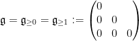
Definition 2 (Host-Kra groups) Let
is the subgroup of
generated by the elements
with
, where
is equal to
and equal to
otherwise.
From construction we see that the Host-Kra group is symmetric with respect to the symmetry group 
Example 3 Let us parameterise an element of
as
. Then
is generated by elements of the form
for
,
and
, and
for
. (This does not cover all the possible faces of
, but it is easy to see that the remaining faces are redundant.) In other words,
, where
, and
. This example is generalised in the exercise below.
Exercise 3 Define a lower face to be a face of a discrete cube
. Let us order the lower faces as
in such a way that
whenever
is a subface of
. Let
be a filtered group. Show that every element of
, where
and the product is taken from left to right (say).
Exercise 4 If
defined in Definition 2 agrees with the group defined at the beginning of this section for additive groups (after transcribing the former to multiplicative notation).
Exercise 5 Let
in an obvious manner, we then obtain a restriction homomorphism from
. Show that the restriction of any element of
then lies in
.
Exercise 6 Let
be integers, and let
and
be elements of
be the element of
defined by setting
for
to equal
for
, and equal to
otherwise. Show that
if and only if
and
, where
is defined in Example 2. (Hint: use Exercises 3, 5.)
Exercise 7 Let
, and let
in the first variable to be the tuple
. Show that
lies in
and
lies in
, where
is defined in Example 2.
Remark 1 The the Host-Kra groups of a filtered group in fact form a cubic complex, a concept used in topology; but we will not pursue this connection here.
In analogy with Exercise 1, we can now define the general notion of a polynomial map:
Definition 3 A map
is said to be polynomial if it maps
to
.
Since 
Theorem 4 (Lazard-Leibman theorem)
(From our choice of definitions, this theorem is a triviality, but the theorem is less trivial when using an alternate but non-trivially equivalent definition of a polynomial, which we will give shortly.) In a similar spirit, we have
Theorem 5 (Filtered groups and polynomial maps form a category) If
are polynomial maps between filtered groups
, then
is also a polynomial map.
We can also give some basic examples of polynomial maps. Any constant map from 


Now we turn to an alternate definition of a polynomial map. For any 


Theorem 6 (Alternate description of polynomials) Let
,
, and
for
, one has
.
In particular, from Exercise 1, we see that a non-classical polynomial of degree 

for all 
Proof: We first prove the “only if” direction. It is clear (by using 


Now we establish the “if” direction. We need to show that 
Let 


By telescoping series, it suffices to establish this when 


Exercise 8 Let
be integers. If
to be the subgroup of
, where
are the coordinates of
. Show that if
to
Exercise 9 Suppose that
from one additive group to another. Show that
to
for every
. Conclude in particular that the composition of a non-classical polynomial of degree
is a non-classical polynomial of degree
.
Exercise 10 Let
,
be non-classical polynomials of degrees
,
respectively between additive groups
, and let
be a bihomomorphism to another additive group (i.e.
is a homomorphism in each variable separately). Show that
is a non-classical polynomial of degree
.
— 2. Nilsequences —
We now specialise the above theory of polynomial maps 


We refer to sequences 


Exercise 11 Let
be an integer, and let
for all
and some
for
, where
. Furthermore, show that the
are unique. We refer to the
as the Taylor coefficients of

Exercise 12 In a degree
nilpotent group
for all
and
explicitly in the form (1).
![\displaystyle g^n h^n = (gh)^n [g,h]^{-\binom{n}{2}}](https://s0.wp.com/latex.php?latex=%5Cdisplaystyle++g%5En+h%5En+%3D+%28gh%29%5En+%5Bg%2Ch%5D%5E%7B-%5Cbinom%7Bn%7D%7B2%7D%7D&bg=ffffff&fg=000000&s=0&c=20201002)
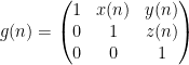
Define a nilpotent filtered Lie group of degree 


(i.e. the group of upper-triangular unipotent matrices with arbitrary real entries in the upper triangular positions) with
and 
Exercise 13 Show that a sequence
from
to the Heisenberg group
are linear polynomials and
is a quadratic polynomial.
It is a standard fact in the theory of Lie groups that a connected, simply connected nilpotent Lie group 


with the inclusions ![{[{\mathfrak g}_i, {\mathfrak g}_j] \subset {\mathfrak g}_{i+j}}](https://s0.wp.com/latex.php?latex=%7B%5B%7B%5Cmathfrak+g%7D_i%2C+%7B%5Cmathfrak+g%7D_j%5D+%5Csubset+%7B%5Cmathfrak+g%7D_%7Bi%2Bj%7D%7D&bg=ffffff&fg=000000&s=0&c=20201002)
and

From the filtration property, we see that for 


We thus see that nilpotent filtered Lie groups are generalisations of vector spaces (which correspond to the degree 


Exercise 14 Let
and
, and let
. Show that the subgroup
of
is a rational number; this may help explain the terminology “rational”.
By hypothesis, the quotient space 


is an extension of the two-dimensional torus 

Every torus of some dimension ![{[0,1]^d}](https://s0.wp.com/latex.php?latex=%7B%5B0%2C1%5D%5Ed%7D&bg=ffffff&fg=000000&s=0&c=20201002)
Exercise 15 Let
for all
, show that for almost all
, that
has exactly one representation of the form
with
, which is given by the identity
where
is the greatest integer part of
, and
is the fractional part function. Conclude that
quotiented by the identifications
between opposite faces.
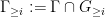
Note that by using the projection
, we can view the Heisenberg nilmanifold
, with the fibers being isomorphic to the unit circle
. (Hint: show that there are some non-trivial homotopies between loops that force the fundamental group of
.)
![\displaystyle [x,y,z] := \begin{pmatrix} 1 & x & y \\ 0 & 1 & z \\ 0 & 0 & 1 \end{pmatrix} \Gamma \in G/\Gamma](https://s0.wp.com/latex.php?latex=%5Cdisplaystyle++%5Bx%2Cy%2Cz%5D+%3A%3D+%5Cbegin%7Bpmatrix%7D+1+%26+x+%26+y+%5C%5C+0+%26+1+%26+z+%5C%5C+0+%26+0+%26+1+%5Cend%7Bpmatrix%7D+%5CGamma+%5Cin+G%2F%5CGamma&bg=ffffff&fg=000000&s=0&c=20201002)
![\displaystyle [x,y,z] = [ \{x\}, \{ y - x \lfloor z \rfloor \}, \{z\} ]](https://s0.wp.com/latex.php?latex=%5Cdisplaystyle++%5Bx%2Cy%2Cz%5D+%3D+%5B+%5C%7Bx%5C%7D%2C+%5C%7B+y+-+x+%5Clfloor+z+%5Crfloor+%5C%7D%2C+%5C%7Bz%5C%7D+%5D&bg=ffffff&fg=000000&s=0&c=20201002)

The logarithm 


![{[e_i,e_j]}](https://s0.wp.com/latex.php?latex=%7B%5Be_i%2Ce_j%5D%7D&bg=ffffff&fg=000000&s=0&c=20201002)
![\displaystyle [e_i,e_j] = \sum_{k=1}^d c_{ijk} e_k.](https://s0.wp.com/latex.php?latex=%5Cdisplaystyle++%5Be_i%2Ce_j%5D+%3D+%5Csum_%7Bk%3D1%7D%5Ed+c_%7Bijk%7D+e_k.&bg=ffffff&fg=000000&s=0&c=20201002)
The structure constants 


A polynomial orbit in a filtered nilmanifold 


Exercise 16 For any
, show that the sequence
(using the notation from Exercise 15) is a polynomial sequence in the Heisenberg nilmaniofold.
![\displaystyle n \mapsto [ \{ -\alpha n \}, \{ \alpha n \lfloor \beta n \rfloor \}, \{ \beta n \} ]](https://s0.wp.com/latex.php?latex=%5Cdisplaystyle++n+%5Cmapsto+%5B+%5C%7B+-%5Calpha+n+%5C%7D%2C+%5C%7B+%5Calpha+n+%5Clfloor+%5Cbeta+n+%5Crfloor+%5C%7D%2C+%5C%7B+%5Cbeta+n+%5C%7D+%5D&bg=ffffff&fg=000000&s=0&c=20201002)
With the above example, we see the emergence of bracket polynomials when representing polynomial orbits in a fundamental domain. Indeed, one can view the entire machinery of orbits in nilmanifolds as a means of efficiently capturing such polynomials in an algebraically tractable framework (namely, that of polynomial sequences in nilpotent groups). The piecewise continuous nature of the bracket polynomials is then ultimately tied to the twisted gluing needed to identify the fundamental domain with the nilmanifold.
Finally, we can define the notion of a (basic Lipschitz) nilsequence of degree 

A basic example of a degree 


or more generally

are also degree 
![{\psi: [0,1] \rightarrow {\bf C}}](https://s0.wp.com/latex.php?latex=%7B%5Cpsi%3A+%5B0%2C1%5D+%5Crightarrow+%7B%5Cbf+C%7D%7D&bg=ffffff&fg=000000&s=0&c=20201002)


The only degree 

Exercise 17 Show that a degree
depending only on
Exercise 18 Show that the class of nilsequences of degree
, or if we add the additional condition
.
Remark 2 The space of nilsequences is also unchanged if one insists that the polynomial orbit be linear, and that the filtration be the lower central series filtration; and this is in fact the original definition of a nilsequence. The proof of this equivalence is a little tricky, though, and will appear in a forthcoming paper of Green, Ziegler, and myself.
— 3. Connection with the Gowers norms —
We define the Gowers norm ![{\|f\|_{U^d[N]}}](https://s0.wp.com/latex.php?latex=%7B%5C%7Cf%5C%7C_%7BU%5Ed%5BN%5D%7D%7D&bg=ffffff&fg=000000&s=0&c=20201002)
![{f: [N] \rightarrow {\bf C}}](https://s0.wp.com/latex.php?latex=%7Bf%3A+%5BN%5D+%5Crightarrow+%7B%5Cbf+C%7D%7D&bg=ffffff&fg=000000&s=0&c=20201002)
![\displaystyle \|f\|_{U^d[N]} := \|f\|_{U^d({\bf Z}/N'{\bf Z})} / \|1_{[N]}\|_{U^d({\bf Z}/N'{\bf Z})}](https://s0.wp.com/latex.php?latex=%5Cdisplaystyle++%5C%7Cf%5C%7C_%7BU%5Ed%5BN%5D%7D+%3A%3D+%5C%7Cf%5C%7C_%7BU%5Ed%28%7B%5Cbf+Z%7D%2FN%27%7B%5Cbf+Z%7D%29%7D+%2F+%5C%7C1_%7B%5BN%5D%7D%5C%7C_%7BU%5Ed%28%7B%5Cbf+Z%7D%2FN%27%7B%5Cbf+Z%7D%29%7D&bg=ffffff&fg=000000&s=0&c=20201002)
where 

![{[N]}](https://s0.wp.com/latex.php?latex=%7B%5BN%5D%7D&bg=ffffff&fg=000000&s=0&c=20201002)


![{\|1_{[N]}\|_{U^d({\bf Z}/N'{\bf Z})}}](https://s0.wp.com/latex.php?latex=%7B%5C%7C1_%7B%5BN%5D%7D%5C%7C_%7BU%5Ed%28%7B%5Cbf+Z%7D%2FN%27%7B%5Cbf+Z%7D%29%7D%7D&bg=ffffff&fg=000000&s=0&c=20201002)

One of the main reasons why nilsequences are relevant to the theory of the Gowers norms is that they are an obstruction to that norm being small. More precisely, we have
Theorem 7 (Converse to the inverse conjecture for the Gowers norms) Let
and
for some degree
.
We now prove this theorem, following an argument of Green, Ziegler, and myself. It is convenient to introduce a few more notions. Define a vertical character of a degree 


for all 

For instance, a polynomial phase 

Exercise 19 Show that a degree
for some
and
A basic fact (generalising the invertibility of the Fourier transform in the degree
Exercise 20 Show that any degree
More quantitatively, show that a degree
can be approximated uniformly to error
by a sum of
nilsequences, each with a representation with a vertical frequency that is of complexity
A derivative 
Lemma 8 (Differentiating nilsequences with a vertical frequency) Let
, and let
be a degree
,
is a degree
.
Proof: We just prove the first claim, as the second claim follows by refining the argument.
We write 


where 
and 

Now we give a filtration on 

for 


Next, we use the hypothesis that 


where 

We now prove Theorem 7 by induction on 
Let 


(extending
![\displaystyle |\mathop{\bf E}_{n \in [N]} \Delta_h f(n) \overline{\Delta_h \psi(n)}| \gg_\delta 1](https://s0.wp.com/latex.php?latex=%5Cdisplaystyle++%7C%5Cmathop%7B%5Cbf+E%7D_%7Bn+%5Cin+%5BN%5D%7D+%5CDelta_h+f%28n%29+%5Coverline%7B%5CDelta_h+%5Cpsi%28n%29%7D%7C+%5Cgg_%5Cdelta+1&bg=ffffff&fg=000000&s=0&c=20201002)
for 
![{h \in [-N,N]}](https://s0.wp.com/latex.php?latex=%7Bh+%5Cin+%5B-N%2CN%5D%7D&bg=ffffff&fg=000000&s=0&c=20201002)
![\displaystyle \| \Delta_h f\|_{U^s[N]} \gg_{\delta, M} 1](https://s0.wp.com/latex.php?latex=%5Cdisplaystyle++%5C%7C+%5CDelta_h+f%5C%7C_%7BU%5Es%5BN%5D%7D+%5Cgg_%7B%5Cdelta%2C+M%7D+1&bg=ffffff&fg=000000&s=0&c=20201002)
for
we close the induction and obtain the claim.
In the other direction, we have
Theorem 9 (Inverse conjecture for the Gowers norms on
. Then
for some degree
.
This conjecture has recently been proven by Green, Ziegler, and myself; an announcement of this result, which will contain extensive heuristic discussion of how this conjecture is proven, will appear very shortly, and the paper itself soon after that. For a discussion of the history of the conjecture, including the cases 
Exercise 21 (
inverse theorem)
- (Straightening an approximately linear function) Let
. Let
be a function such that
for all but
of all
with
. If
with
such that
for all but
values of
, where
as
. (Hint: One can take
to be small. First find a way to lift
in a nice manner from
- Let
. Show that there exists a polynomial
, where
as
The inverse conjecture for the Gowers norms, when combined with the equidistribution theory for nilsequences that we will turn to next, has a number of consequences, analogous to the consequences for the finite field analogues of these facts; see this paper of Green and myself for further discussion.
— 4. Equidistribution of nilsequences —
In the subject of higher order Fourier analysis, and in particular in the proof of the inverse conjecture for the Gowers norms, as well as in several of the applications of this conjecture, it will be of importance to be able to compute statistics of nilsequences ![{\mathop{\bf E}_{n \in [N]} \psi(n)}](https://s0.wp.com/latex.php?latex=%7B%5Cmathop%7B%5Cbf+E%7D_%7Bn+%5Cin+%5BN%5D%7D+%5Cpsi%28n%29%7D&bg=ffffff&fg=000000&s=0&c=20201002)
![{\mathop{\bf E}_{n \in [N]} e(P(n))}](https://s0.wp.com/latex.php?latex=%7B%5Cmathop%7B%5Cbf+E%7D_%7Bn+%5Cin+%5BN%5D%7D+e%28P%28n%29%29%7D&bg=ffffff&fg=000000&s=0&c=20201002)


![\displaystyle \lim_{N \rightarrow \infty} \mathop{\bf E}_{n \in [N]} F({\mathcal O}(n)) = 0](https://s0.wp.com/latex.php?latex=%5Cdisplaystyle++%5Clim_%7BN+%5Crightarrow+%5Cinfty%7D+%5Cmathop%7B%5Cbf+E%7D_%7Bn+%5Cin+%5BN%5D%7D+F%28%7B%5Cmathcal+O%7D%28n%29%29+%3D+0&bg=ffffff&fg=000000&s=0&c=20201002)
for all Lipschitz
When studying equidistribution of polynomial sequences in a torus 


The notion of a derivative requires the ability to perform subtraction on the range space 


Lemma 10 (Relative van der Corput lemma) Let
be a sequence in a degree
is asymptotically equidistributed, and suppose also that for each non-zero
is asymptotically equidistributed with respect to some
on
. Then
Proof: It suffices to show that, for each Lipschitz function
![\displaystyle \lim_{n \rightarrow \infty} \mathop{\bf E}_{n \in [N]} F(x(n)) = \int_{G/\Gamma} F\ d\mu_{G/\Gamma}.](https://s0.wp.com/latex.php?latex=%5Cdisplaystyle++%5Clim_%7Bn+%5Crightarrow+%5Cinfty%7D+%5Cmathop%7B%5Cbf+E%7D_%7Bn+%5Cin+%5BN%5D%7D+F%28x%28n%29%29+%3D+%5Cint_%7BG%2F%5CGamma%7D+F%5C+d%5Cmu_%7BG%2F%5CGamma%7D.&bg=ffffff&fg=000000&s=0&c=20201002)
By Exercise 20, we may assume that 
![\displaystyle \lim_{n \rightarrow \infty} \mathop{\bf E}_{n \in [N]} F(x(n+h)) \overline{F(x(n))} = 0](https://s0.wp.com/latex.php?latex=%5Cdisplaystyle++%5Clim_%7Bn+%5Crightarrow+%5Cinfty%7D+%5Cmathop%7B%5Cbf+E%7D_%7Bn+%5Cin+%5BN%5D%7D+F%28x%28n%2Bh%29%29+%5Coverline%7BF%28x%28n%29%29%7D+%3D+0&bg=ffffff&fg=000000&s=0&c=20201002)
for each non-zero 


![\displaystyle \lim_{n \rightarrow \infty} \mathop{\bf E}_{n \in [N]} F(x(n+h)) \overline{F(x(n))} = \int_{(G/\Gamma \times G/\Gamma)/T^\Delta} \tilde F\ d\mu_h.](https://s0.wp.com/latex.php?latex=%5Cdisplaystyle++%5Clim_%7Bn+%5Crightarrow+%5Cinfty%7D+%5Cmathop%7B%5Cbf+E%7D_%7Bn+%5Cin+%5BN%5D%7D+F%28x%28n%2Bh%29%29+%5Coverline%7BF%28x%28n%29%29%7D+%3D+%5Cint_%7B%28G%2F%5CGamma+%5Ctimes+G%2F%5CGamma%29%2FT%5E%5CDelta%7D+%5Ctilde+F%5C+d%5Cmu_h.&bg=ffffff&fg=000000&s=0&c=20201002)
The function 
This gives a useful criterion for equidistribution of polynomial orbits. Define a horizontal character to be a continuous homomorphism ![{G/([G,G]\Gamma)}](https://s0.wp.com/latex.php?latex=%7BG%2F%28%5BG%2CG%5D%5CGamma%29%7D&bg=ffffff&fg=000000&s=0&c=20201002)

Theorem 11 (Leibman equidistribution criterion) Let
be a polynomial orbit on a degree
. Then
is non-constant for each non-trivial horizontal character.
This theorem was first established by Leibman (by a slightly different method), and also follows from the above van der Corput lemma and some tedious additional computations; see this paper of Green and myself for details. For linear orbits, this result was established by Parry and by Leon Green. Using this criterion (together with more quantitative analogues for single-scale equidistribution), one can develop Ratner-type decompositions that generalise those in (Notes 1). Again, the details are technical and I refer to my paper with Green for details. We give a special case of Theorem 11 as an exercise:
Exercise 22 Use Lemma 10 to show that if
are two real numbers such that
are linearly independent modulo
is asymptotically equidistributed in the Heisenberg nilmanifold
is asymptotically equidistributed in the unit circle.

Unfortunately Lemma 10 is not strong enough to cover all cases of Theorem 11; in particular, if 

One application of this equidistribution theory is to show that bracket polynomial objects such as (2) have a negligible correlation with any genuinely quadratic phase 
![{U^3[N]}](https://s0.wp.com/latex.php?latex=%7BU%5E3%5BN%5D%7D&bg=ffffff&fg=000000&s=0&c=20201002)

Exercise 23 Let the notation be as in Exercise 22. Show that
for any
. (You can either apply Theorem 11, or go back to Lemma 10.)
![\displaystyle \lim_{n \rightarrow\infty} \mathop{\bf E}_{n \in [N]} e( \alpha n \lfloor \beta n \rfloor - \gamma n^2 - \delta n ) = 0](https://s0.wp.com/latex.php?latex=%5Cdisplaystyle++%5Clim_%7Bn+%5Crightarrow%5Cinfty%7D+%5Cmathop%7B%5Cbf+E%7D_%7Bn+%5Cin+%5BN%5D%7D+e%28+%5Calpha+n+%5Clfloor+%5Cbeta+n+%5Crfloor+-+%5Cgamma+n%5E2+-+%5Cdelta+n+%29+%3D+0&bg=ffffff&fg=000000&s=0&c=20201002)

11 comments
Comments feed for this article
30 May, 2010 at 10:47 am
Bogdan
Dear Professor Tao
Am I correct that Theorem 9 (Inverse conjecture for the Gowers norms on Z) is exactly the same conjecture mentioned in the paper “Linear equations in primes”, and thus that results are now fully unconditional?
30 May, 2010 at 11:06 pm
Terence Tao
It is equivalent to the conjecture formulated there, yes. We’re preparing a formal announcement of the results which should appear here within a week or so, and the full paper should be ready shortly afterwards.
4 June, 2010 at 1:24 pm
Jingzheng
Dear Professor Tao
Inverse conjecture for Gowers norms roughly says for example that if a bounded function f does not resemble a nilsequence then the sum of terms f(a)g(a+b)h(a+2b)k(a+3b) (for a, b from suitable ranges and g,h,k bounded) is of smaller order than the magnitude resulting from estimating trivially. Are there any partial results or conjectures concerning nonlinear equations? For instance: is there any conjecture about sum of f(a)g(d)h(b)k(c) over quadruples (a,b,c,d) satisfying ad-bc=1? If this sum is as large as possible then what are the functions that f,g,h and k must resemble?
4 June, 2010 at 1:46 pm
Terence Tao
This is an important question, but not much is known presently, even in the simplest example of nonlinearity, namely averages over polynomials. If one is working in a finite field, and all parameters range freely in this field, then one can usually use a version of the van der Corput inequality (combined with PET induction) to control things by Gowers norms. But over an interval of integers [N], the problem once one has nonlinearity is that some of the parameters now need to be restricted to smaller intervals, such as [N^{1/d}] for some d. In some cases one can still hope to control things by “local” Gowers norms – Tamar Ziegler and I did something like this for instance when finding polynomial progressions in primes. But the general situation is still quite murky. I suspect that some of the theory from sum-product estimates and expansion in linear groups may have to come into play, particularly for patterns such as ad-bc=1 that are clearly connected to linear groups such as SL_2.
4 June, 2010 at 2:06 pm
Jingzheng
Dear Professor Tao
Thank you for the answer. Your mentioning of the paper with dr Ziegler about polynomial progressions of primes reminded me of another interesting problem. Since the progressions of length at least 4 involve as complicated objects as nilsequences then in order to try to find an asymptotics for polynomial progressions maybe it is appropriate first to investigate asymptotics for polynomial progressions of length 3? The simplest nontrivial case would be: a, a+b^2, a+2b^2. A relevant question here would be: is it true that if the sum of terms f(a)g(a+b^2)h(a+2b^2) is of magnitude N^(3/2) where a is of order N and b is of order N^(1/2) then necessarily f has a large Fourier coefficient?
4 June, 2010 at 3:25 pm
Terence Tao
Yes, something like this should be true (but perhaps one has to deal with a local Fourier coefficient rather than a global one), but this has not been proved yet as far as I know (this would correspond to a polynomial version of a conjecture of Gowers and Wolf, which has only been proven so far in the linear case). There is an ergodic counterpart to your question to which the answer is affirmative, thanks to the work of Bergelson, Leibman, and Lesigne, so heuristically the same should be true for the finitary version of the question, but unfortunately the correspondence principle does not seem to yield this directly.
If one applies the Cauchy-Schwarz inequality enough times, I believe one can control the above sum by something like the (local) U^7 norm of f, which suggests that f will at least correlate with a 6-step nilsequence, but one presumably do better than this with more work.
4 June, 2010 at 3:31 pm
Anonymous
陶教授
我非常感谢您回答
晶正
25 October, 2012 at 10:11 am
Walsh’s ergodic theorem, metastability, and external Cauchy convergence « What’s new
[…] some (standard) finite number of group elements of ; see e.g. Exercise 11 of this previous blog post. In the abelian case, we used the largest for which was non-trivial as the degree of . This turns […]
24 February, 2013 at 1:52 am
pavel zorin
Dear Terry, (these are linearly independent mod 1 over Z because
  is irreducible over Z, say by Cohn’s criterion in base 3). Then
it seems that the relative van der Corput lemma 10 does not apply directly in Exercise 22 (Exercise 1.6.22 in the book draft). Consider the following example:
Hence .
. -invariant then also the closure of the orbit
 would be
  -invariant since
  is central and multiplication by a constant is a homeomorphism. However, this closure is contained in the diagonal of
  .
.
If the closure of this orbit was
best regards,
pavel
24 February, 2013 at 7:53 pm
Terence Tao
Gah, you’re right, this particular argument only works under the stronger hypothesis that are linearly independent. (In the example you gave, one does not have equidistribution for any fixed h, though in some sense the orbits become asymptotically equidistributed as h becomes large, though it is hard to formalise this at the qualitative level.) It seems that to handle the general case one has to either use a quantitative (single-scale) version of the van der Corput lemma (as was done in my paper with Ben) or else rely on the ergodic theorem (this is the approach in Leibman).
27 March, 2013 at 7:34 pm
An informal version of the Furstenberg correspondence principle | What's new
[…] the cost of turning the observable into a slightly messy piecewise smooth function; see e.g. this blog post for details. More generally, any function arising from phases that are bracket polynomials (or […]