As is now widely reported, the Fields medals for 2010 have been awarded to Elon Lindenstrauss, Ngo Bao Chau, Stas Smirnov, and Cedric Villani. Concurrently, the Nevanlinna prize (for outstanding contributions to mathematical aspects of information science) was awarded to Dan Spielman, the Gauss prize (for outstanding mathematical contributions that have found significant applications outside of mathematics) to Yves Meyer, and the Chern medal (for lifelong achievement in mathematics) to Louis Nirenberg. All of the recipients are of course exceptionally qualified and deserving for these awards; congratulations to all of them. (I should mention that I myself was only very tangentially involved in the awards selection process, and like everyone else, had to wait until the ceremony to find out the winners. I imagine that the work of the prize committees must have been extremely difficult.)
Today, I thought I would mention one result of each of the Fields medalists; by chance, three of the four medalists work in areas reasonably close to my own. (Ngo is rather more distant from my areas of expertise, but I will give it a shot anyway.) This will of course only be a tiny sample of each of their work, and I do not claim to be necessarily describing their “best” achievement, as I only know a portion of the research of each of them, and my selection choice may be somewhat idiosyncratic. (I may discuss the work of Spielman, Meyer, and Nirenberg in a later post.)
— 1. Elon Lindenstrauss —
Elon Lindenstrauss works primarily in ergodic theory and dynamical systems, particularly with regard to the homogeneous dynamics of the action of some subgroup  of a Lie group
  on a quotient
  , and on the applications of this theory to questions in analytic number theory.
One of the themes of modern mathematics is that within any field of mathematics, there is some sort of underlying action by a group (or group-like object) which endows certain key objects of study in that field with a rich, symmetric structure (both algebraic and geometric). Analytic number theory is no exception to this; many classical questions, for instance, about Minkowski’s geometry of numbers, Diophantine approximation, or quadratic forms can be interpreted through this modern perspective as questions about the actions of groups such as  on spaces such as the homogeneous space
  . In particular, the dynamical properties of such actions (e.g. the behaviour of orbits, the classification of invariant measures, the mixing properties of the action, or averages of the action) often have direct bearing on the number-theoretic properties of these objects. A typical example of this is the resolution of the Oppenheim conjecture on quadratic forms by Margulis, using a classification of orbit closures in the homogeneous space
  of a certain subgroup
  of
of  , which is also a special case of Ratner’s theorems; this was discussed earlier on this blog at this writeup of a lecture of Margulis, or at this discussion of Ratner’s theorems. Indeed, even though the Oppenheim conjecture is a purely number-theoretic statement, the only known proofs of this conjecture in full generality proceed via homogeneous dynamics. (There are however more number-theoretic proofs of partial cases of this conjecture.)
Another demonstration of this principle is the remarkable 2006 paper of Einsiedler, Katok, and Lindenstrauss that gives the best partial result known to date on the notorious Littlewood conjecture, which asserts that for any real numbers  , and any
  , one can find a positive integer
  such that
  , where
  is the distance from
  to the nearest integer. Note that the Dirichlet approximation theorem already gives
  for infinitely many , and
  is clearly bounded, so the conjecture is tantalisingly close to being “easy”; nevertheless, it has defied proof for about eight decades now.
Einsiedler, Katok, and Lindenstrauss establish the partial result that the Littlewood conjecture is true for “most”  , in the sense that the set of pairs
  for which the conjecture fails is a subset of
  of Hausdorff dimension zero. This is a much stronger statement than the fact that the Littlewood conjecture holds for almost every , which is fairly easy to prove; being dimension zero is much stronger than having measure zero.
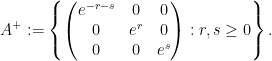
How is this connected with homogeneous dynamics? Fix , and let us consider the orbit  of a point in the homogeneous space

where is given as
and  is the semigroup
The space has finite volume, but is non-compact, having a “cusp” at infinity. Thus, the orbit need not be bounded, but could wander arbitrarily close to the cusp. The connection with the Littlewood conjecture (first observed, I believe, by Margulis) is then
Lemma 1 The Littlewood conjecture is true for if and only if is unbounded.
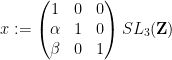
Proof: We’ll just prove the “if” part; the “only if” part is proven by a slightly more sophisticated version of the arguments below. One can identify with the space of all unimodular lattices in  , by identifying each point
  of with the lattice
  . The non-compactness of this space arises from the fact that the shortest non-zero vector in such lattices can become arbitrarily small (or to put it contrapositively, as long as one keeps the non-zero vectors of a unimodular lattice away from zero, the space of such lattices becomes (pre)compact). In particular, is unbounded if and only if the vector

where  and
and  are integers not all zero, can become arbitrarily small. We can multiply out this vector as
We conclude that if is unbounded, then for any , we can find and (not all zero) such that

Since and are not all zero, we easily verify that this forces to be non-zero if  is small enough. Multiplying all three terms together, we obtain

which simplifies to

But the left-hand side is at least  , we conclude that Littlewood’s conjecture is true for as required.
The orbits of semigroups such as are still not well understood, in contrast to the orbits of unipotently generated groups for which we have the powerful theorems of Ratner. Nevertheless, by a remarkable analysis of the effects of hyperbolicity on the entropy of an invariant measure, Einsiedler, Katok, and Lindenstrauss are able to obtain some general theorems concerning invariant measures of such semigroups which gives the above consequence to Littlewood’s conjecture, as well as many other applications.
— 2. Ngo Bao Chau —
(Caveat: my understanding of the subject matter here is rather superficial, and so what I write below may be somewhat inaccurate in places. Corrections and clarifications would, of course, be greatly appreciated!)
Ngo Bao Chau has made major contributions to the Langlands programme, which among other things seeks to control the automorphic representations of a (connected, reductive) algebraic group by the Langlands dual group  , in a way which is analogous to how the representation theory of a (locally compact) abelian group is controlled by the Pontryagin dual group
  . Thus, the Langlands programme can be viewed in some sense as a generalisation of Fourier analysis to non-abelian groups . For instance, the classical Poisson summation formula, that relates summations in an abelian group to summations in its Pontryagin dual , has a vast generalisation in the Selberg trace formula and its generalisations (in particular, the Arthur-Selberg trace formula), which very roughly speaking relates summations (of orbital integrals) over conjugacy classes in with sums over the automorphic representations of (which, by Langlands duality, should be in turn controlled somehow by ).
The Poisson summation formula is closely related to the “functorial” properties of the Fourier transform  : every homomorphism
  of locally compact abelian groups induces a corresponding adjoint homomorphism
  on the Pontryagin dual groups, and one can interpret Poisson summation as being a consequence of the claim that pullback by the homomorphism
  becomes pushforward by the adjoint homomorphism
  after taking Fourier transforms. As I understand it (which is, admittedly, not very well), Langlands functoriality is a nonabelian generalisation of this Fourier functoriality. However, the notions of pushforward and pullback become much more complicated in the nonabelian world, as one is working on things such as conjugacy classes and representations, rather than individual elements of the groups involved. One can define these notions relatively easily in a “local” fashion, working one place at a time, but to glue everything together properly into a “global” setting (in which one is working over an adele ring) in such a way that the relevant trace formulae remain compatible requires the fundamental lemma, the establishment of which was then a major goal of the Langlands programme (as it makes the trace formula significantly more useful, particularly for applications to number theory). In 2008, Ngo established this lemma in full generality, building upon several special cases and previous reductions by other mathematicians (including an earlier breakthrough paper of Laumon and Ngo), and also importing a major new tool from geometry and mathematical physics, namely that of a Hitchin fibration. Apparently, a key observation of Ngo is that the sums over conjugacy classes that appear in the trace formula can be naturally interpreted in terms of some geometric data associated to such fibrations. This is a deep connection which not only gives the fundamental lemma (after a lot of difficult work), but gives a better understanding as to the Langlands programme as a whole.
— 3. Stas Smirnov —
Stas Smirnov works in a number of related fields, and in particular in complex dynamics and in statistical physics. One of his celebrated results in the latter area is the first rigorous demonstration of conformal invariance for a scaling limit percolation model, namely that of percolation on the triangular lattice; this invariance was conjectured for physicists for some time (being part of a larger philosophy of universality, that asserts that the large-scale behaviour of a statistical system should be largely insensitive to the precise small-scale geometry of that system, after normalising some key parameters). Smirnov’s result, especially when combined with the theory of the Schramm-Loewner equation (SLE) developed by Lawler, Schramm, and Werner which classifies conformally invariant processes, allows for a rigorous analysis of many random processes in statistical physics, confirming the general intuition of universality, although the underlying explanation for the universality phenomenon is still lacking. (For instance, we still do not have an analogue of Stas’s result for any lattice other than the triangular one.) Note that this universality phenomenon is not directly related to the universality phenomenon observed in random matrix theory (which has guided much of my own recent research with Van Vu), though there are certainly some superficial similarities between the two.
Smirnov’s full result of conformal invariance for the triangular lattice is a bit tricky to state, but it is a bit easier to state a simpler but still highly non-trivial consequence of that result, namely Cardy’s formula for crossing probabilities in the scaling limit. As observed by Carleson, this formula is easiest to state when the domain is a unit equilateral triangle  , though it is an important consequence of Stas’s conformal invariance result (first conjectured by Aizenman) that it can in fact be phrased for any simply connected domain in the plane.
Pick a large natural number , and subdivide the original unit equilateral triangle into  subtriangles of sidelength
  . This creates a triangular lattice on
  (the
(the  triangular number, naturally) vertices or sites. Now randomly colour each site blue and yellow (say), with an independent
  probability of each; this is the critical probability for this lattice, in which neither colour dominates, and thus gives the most interesting behaviour. The site colouring then separates the vertices into blue and yellow clusters, with two vertices of the same colour belonging to the same cluster if they are connected by a path in the lattice that only goes through vertices of that colour.
The size, shape, and other geometrical properties of clusters in such lattice models, especially in the scaling limit  , is the main subject of study of percolation theory. There are many such aspects to this theory, but let us focus on a relatively simple aspect, namely the crossing probability between two line segments on the boundary of the triangle , say
  and
and  , where
  is a site on the line segment
  . This crossing probability is defined to be the probability that there is a blue (say) cluster connecting with , or equivalently that there is a blue path that starts at and ends at . Clearly, for fixed , this probability is an increasing function of the length
  of the line segment , which equals
  when is equal to
  , and which we expect to be close to zero at the other extreme when is equal to
  . Cardy’s formula is the assertion that in the limit
  , the crossing probability is asymptotically equal to the length of the interval. (There is a similar formula when one replaces the triangle by a more general simply connected domain (while still keeping the small-scale triangular lattice structure), and replaces and by two arcs on the boundary of that domain, but then one has to apply the Riemann mapping theorem to convert that domain back into the equilateral triangle.)
The first step in Smirnov’s proof of Cardy’s formula is to consider a two-dimensional extension of the crossing probability, namely the function  defined for
  in the solid triangle , defined as the probability that there is a blue path from to that separates from
  . Note that when is a boundary point on the edge , then is basically the crossing probability from to (ignoring some boundary effects which are negligible in the asymptotic limit ); thus the crossing probability arises as the boundary values of
  . Smirnov was able to show that the function is asymptotically harmonic and obeys some natural Dirichlet-Neumann boundary conditions, which ultimately gives Cardy’s formula. By pushing this analysis much further, these methods also eventually give the conformal invariance of the entire triangular lattice percolation process.
— 4. Cedric Villani —
Cedric Villani works in several areas of mathematical physics, and particularly in the rigorous theory of continuum mechanics equations such as the Boltzmann equation.
Imagine a gas consisting of a large number of particles traveling at various velocities. To begin with, let us take a ridiculously oversimplified discrete model and suppose that there are only four distinct velocities that the particles can be in, namely  , and
, and  . Let us also make the homogeneity assumption that the distribution of velocities of the gas is independent of the position; then the distribution of the gas at any given time
  can then be described by four densities
  adding up to , which describe the proportion of the gas that is currently traveling at velocities
  , etc..
If there were no collisions between the particles that could transfer velocity from one particle to another, then all the quantities  would be constant in time:
  . But suppose that there is a collision reaction that can take two particles traveling at velocities
  and change their velocities to
  , or vice versa, and that no other collision reactions are possible. Making the key heuristic assumption that different particles are distributed more or less independently in space for the purposes of computing the rate of collision (this hypothesis is also known as the molecular chaos or Stosszahlansatz hypothesis), the rate at which the former type of collision occurs will be proportional to
  , while the rate at which the latter type of collision occurs is proportional to
  . This leads to equations of motion such as

for some rate constant  , and similarly for
  ,
,  , and
, and  . It is interesting to note that even in this simplified model, we see the emergence of an “arrow of time”: the rate of a collision is determined by the density of the initial velocities rather than the final ones, and so the system is not time reversible, despite being a statistical limit of a time-reversible collision from the velocities
  to
to  and vice versa.
To take a less ridiculously oversimplified model, now suppose that particles can take a continuum of velocities, but we still make the homogeneity assumption the velocity distribution is still independent of position, so that the state is now described by a density function  , with
  now ranging continuously over . There are now a continuum of possible collisions, in which two particles of initial velocity
  (say) collide and emerge with velocities
  . If we assume purely elastic collisions between particles of identical mass
  , then we have the law of conservation of momentum

and conservation of energy
some simple Euclidean geometry shows that the pre-collision velocities must be related to the post-collision velocities by the formulae

for some unit vector  . Thus a collision can be completely described by the post-collision velocities
  and the pre-collision direction vector ; assuming Galilean invariance, the physical features of this collision can in fact be described just using the relative post-collision velocity
  and the pre-collision direction vector
  . Using the same independence heuristics used in the four velocities model, we are then led to the equation of motion

where  is the quadratic expression

for some Boltzmann collision kernel  , which depends on the physical nature of the hard spheres, and needs to be specified as part of the dynamics. Here of course are given by (1).
If one now allows the velocity distribution to depend on position  in a domain
  , so that the density function is now
  , then one has to combine the above equation with a transport equation, leading to the Boltzmann equation
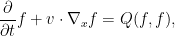
together with some boundary conditions on the spatial boundary  that will not be discussed here.
One of the most fundamental facts about this equation is the Boltzmann H theorem, which asserts that (given sufficient regularity and integrability hypotheses on  , and reasonable boundary conditions), the -functional

is non-increasing in time, with equality if and only if the density function is Gaussian in at each position (but where the mass, mean and variance of the Gaussian distribution being allowed to vary in ). Such distributions are known as Maxwellian distributions.
From a physical perspective, is the negative of the entropy of the system, so the H theorem is a manifestation of the second law of thermodynamics, which asserts that the entropy of a system is non-decreasing in time, thus clearly demonstrating the “arrow of time” mentioned earlier.
There are considerable technical issues in ensuring that the derivation of the H theorem is actually rigorous for reasonable regularity hypotheses on (and on ), in large part due to the delicate and somewhat singular nature of “grazing collisions” when the pre-collision and post-collision velocities are very close to each other. Important work was done by Villani and his co-authors on resolving this issue, but this is not the result I want to focus on here. Instead, I want to discuss the long-time behaviour of the Boltzmann equation.
As the functional always decreases until a Maxwellian distribution is attained, it is then reasonable to conjecture that the density function must converge (in some suitable topology) to a Maxwellian distribution. Furthermore, even though the theorem allows the Maxwellian distribution to be non-homogeneous in space, the transportation aspects of the Boltzmann equation should serve to homogenise the spatial behaviour, so that the limiting distribution should in fact be a homogeneous Maxwellian. In a remarkable 72-page tour de force, Desvilletes and Villani showed that (under some strong regularity assumptions), this was indeed the case, and furthermore the convergence to the Maxwellian distribution was quite fast, faster than any polynomial rate of decay in fact. Remarkably, this was a large data result, requiring no perturbative hypotheses on the initial distribution (although a fair amount of regularity was needed). As is usual in PDE, large data results are considerably more difficult due to the lack of perturbative techniques that are initially available; instead, one has to primarily rely on such tools as conservation laws and monotonicity formulae. One of the main tools used here is a quantitative version of the H theorem (also obtained by Villani), but this is not enough; the quantitative bounds on entropy production given by the H theorem involve quantities other than the entropy, for which further equations of motion (or more precisely, differential inequalities on their rate of change) must be found, by means of various inequalities from harmonic analysis and information theory. This ultimately leads to a finite-dimensional system of ordinary differential inequalities that control all the key quantities of interest, which must then be solved to obtain the required convergence.


67 comments
Comments feed for this article
1 November, 2017 at 1:45 am
Laudationes de las medallas Fields 2010 | Ciencia | La Ciencia de la Mula Francis
[…] técnico de los 4 nuevos Medalla Fields recomiendo la entrada del genial Terence Tao, “Lindenstrauss, Ngo, Smirnov, Villani,” What’s New, 19 August, 2010, que como siempre, lo […]
1 August, 2018 at 9:01 am
Birkar, Figalli, Scholze, Venkatesh | What's new
[…] the two previous congresses in 2010 and 2014, I wrote blog posts describing some of the work of each of the winners. This time, though, I happened to be a […]