
Let ![{[a,b]}](https://s0.wp.com/latex.php?latex=%7B%5Ba%2Cb%5D%7D&bg=ffffff&fg=000000&s=0&c=20201002)
![{F: [a,b] \rightarrow {\bf R}}](https://s0.wp.com/latex.php?latex=%7BF%3A+%5Ba%2Cb%5D+%5Crightarrow+%7B%5Cbf+R%7D%7D&bg=ffffff&fg=000000&s=0&c=20201002)
![{x \in [a,b]}](https://s0.wp.com/latex.php?latex=%7Bx+%5Cin+%5Ba%2Cb%5D%7D&bg=ffffff&fg=000000&s=0&c=20201002)
![\displaystyle F'(x) := \lim_{y \rightarrow x; y \in [a,b] \backslash \{x\}} \frac{F(y)-F(x)}{y-x} \ \ \ \ \ (1)](https://s0.wp.com/latex.php?latex=%5Cdisplaystyle+F%27%28x%29+%3A%3D+%5Clim_%7By+%5Crightarrow+x%3B+y+%5Cin+%5Ba%2Cb%5D+%5Cbackslash+%5C%7Bx%5C%7D%7D+%5Cfrac%7BF%28y%29-F%28x%29%7D%7By-x%7D+%5C+%5C+%5C+%5C+%5C+%281%29&bg=ffffff&fg=000000&s=0&c=20201002)
exists. In that case, we call 


Remark 1 Much later in this sequence, when we cover the theory of distributions, we will see the notion of a weak derivative or distributional derivative, which can be applied to a much rougher class of functions and is in many ways more suitable than the classical derivative for doing “Lebesgue” type analysis (i.e. analysis centred around the Lebesgue integral, and in particular allowing functions to be uncontrolled, infinite, or even undefined on sets of measure zero). However, for now we will stick with the classical approach to differentiation.
Exercise 2 If
Exercise 3 Give an example of a function
, but which also oscillates rapidly near that point.)
In single-variable calculus, the operations of integration and differentiation are connected by a number of basic theorems, starting with Rolle’s theorem.
Theorem 4 (Rolle’s theorem) Let
. Then there exists
such that
.
Proof: By subtracting a constant from 

![{\sup_{x \in [a,b]} F(x) > 0}](https://s0.wp.com/latex.php?latex=%7B%5Csup_%7Bx+%5Cin+%5Ba%2Cb%5D%7D+F%28x%29+%3E+0%7D&bg=ffffff&fg=000000&s=0&c=20201002)

![{y \in [a,b]}](https://s0.wp.com/latex.php?latex=%7By+%5Cin+%5Ba%2Cb%5D%7D&bg=ffffff&fg=000000&s=0&c=20201002)


Remark 5 Observe that the same proof also works if
of the interval
Exercise 6 Give an example to show that Rolle’s theorem can fail if
is merely assumed to be almost everywhere differentiable, even if one adds the additional hypothesis that
Remark 7 It is important to note that Rolle’s theorem only works in the real scalar case when
. If, for instance, we consider complex-valued scalar functions
, then the theorem can fail; for instance, the function
defined by
vanishes at both endpoints and is differentiable, but its derivative
is never zero. (Rolle’s theorem does imply that the real and imaginary parts of the derivative
.
One can easily amplify Rolle’s theorem to the mean value theorem:
Corollary 8 (Mean value theorem) Let
.
Proof: Apply Rolle’s theorem to the function 
Remark 9 As Rolle’s theorem is only applicable to real scalar-valued functions, the more general mean value theorem is also only applicable to such functions.
Exercise 10 (Uniqueness of antiderivatives up to constants) Let
be differentiable functions. Show that
for every
for some constant
and all
We can use the mean value theorem to deduce one of the fundamental theorems of calculus:
Theorem 11 (Second fundamental theorem of calculus) Let
of
. In particular, we have
whenever
Proof: Let 


for every choice of ![{t^*_j \in [t_{j-1},t_j]}](https://s0.wp.com/latex.php?latex=%7Bt%5E%2A_j+%5Cin+%5Bt_%7Bj-1%7D%2Ct_j%5D%7D&bg=ffffff&fg=000000&s=0&c=20201002)
Fix this partition. From the mean value theorem, for each 

and thus by telescoping series
Since
Remark 12 Even though the mean value theorem only holds for real scalar functions, the fundamental theorem of calculus holds for complex or vector-valued functions, as one can simply apply that theorem to each component of that function separately.
Of course, we also have the other half of the fundamental theorem of calculus:
Theorem 13 (First fundamental theorem of calculus) Let
be a continuous function, and let
. Then
for all
Proof: It suffices to show that
for all 

for all ![{x \in (a,b]}](https://s0.wp.com/latex.php?latex=%7Bx+%5Cin+%28a%2Cb%5D%7D&bg=ffffff&fg=000000&s=0&c=20201002)

for any 


![{[0,1]}](https://s0.wp.com/latex.php?latex=%7B%5B0%2C1%5D%7D&bg=ffffff&fg=000000&s=0&c=20201002)


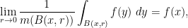
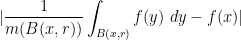
Corollary 14 (Differentiation theorem for continuous functions) Let
for all
for all
for all
![\displaystyle \lim_{h \rightarrow 0^+} \frac{1}{h} \int_{[x,x+h]} f(t)\ dt = f(x)](https://s0.wp.com/latex.php?latex=%5Cdisplaystyle+%5Clim_%7Bh+%5Crightarrow+0%5E%2B%7D+%5Cfrac%7B1%7D%7Bh%7D+%5Cint_%7B%5Bx%2Cx%2Bh%5D%7D+f%28t%29%5C+dt+%3D+f%28x%29&bg=ffffff&fg=000000&s=0&c=20201002)
![\displaystyle \lim_{h \rightarrow 0^+} \frac{1}{h} \int_{[x-h,x]} f(t)\ dt = f(x)](https://s0.wp.com/latex.php?latex=%5Cdisplaystyle+%5Clim_%7Bh+%5Crightarrow+0%5E%2B%7D+%5Cfrac%7B1%7D%7Bh%7D+%5Cint_%7B%5Bx-h%2Cx%5D%7D+f%28t%29%5C+dt+%3D+f%28x%29&bg=ffffff&fg=000000&s=0&c=20201002)
![\displaystyle \lim_{h \rightarrow 0^+} \frac{1}{2h} \int_{[x-h,x+h]} f(t)\ dt = f(x)](https://s0.wp.com/latex.php?latex=%5Cdisplaystyle+%5Clim_%7Bh+%5Crightarrow+0%5E%2B%7D+%5Cfrac%7B1%7D%7B2h%7D+%5Cint_%7B%5Bx-h%2Cx%2Bh%5D%7D+f%28t%29%5C+dt+%3D+f%28x%29&bg=ffffff&fg=000000&s=0&c=20201002)
In these notes we explore the question of the extent to which these theorems continue to hold when the differentiability or integrability conditions on the various functions 
- The Lebesgue differentiation theorem, which roughly speaking asserts that Corollary 14 continues to hold for almost every
- A number of differentiation theorems, which assert for instance that monotone, Lipschitz, or bounded variation functions in one dimension are almost everywhere differentiable; and
- The second fundamental theorem of calculus for absolutely continuous functions.
The material here is loosely based on Chapter 3 of Stein-Shakarchi.
— 1. The Lebesgue differentiation theorem in one dimension —
The main objective of this section is to show
Theorem 15 (Lebesgue differentiation theorem, one-dimensional case) Let
be an absolutely integrable function, and let
be the definite integral
. Then
for almost every
.
This can be viewed as a variant of Corollary 14; the hypotheses are weaker because ![{f = 1_{[0,1]}}](https://s0.wp.com/latex.php?latex=%7Bf+%3D+1_%7B%5B0%2C1%5D%7D%7D&bg=ffffff&fg=000000&s=0&c=20201002)
The continuity is an easy exercise:
Exercise 16 Let
The main difficulty is to show that 
Theorem 17 (Lebesgue differentiation theorem, second formulation) Let
for almost every
![\displaystyle \lim_{h \rightarrow 0^+} \frac{1}{h} \int_{[x,x+h]} f(t)\ dt = f(x) \ \ \ \ \ (2)](https://s0.wp.com/latex.php?latex=%5Cdisplaystyle+%5Clim_%7Bh+%5Crightarrow+0%5E%2B%7D+%5Cfrac%7B1%7D%7Bh%7D+%5Cint_%7B%5Bx%2Cx%2Bh%5D%7D+f%28t%29%5C+dt+%3D+f%28x%29+%5C+%5C+%5C+%5C+%5C+%282%29&bg=ffffff&fg=000000&s=0&c=20201002)
![\displaystyle \lim_{h \rightarrow 0^+} \frac{1}{h} \int_{[x-h,x]} f(t)\ dt = f(x) \ \ \ \ \ (3)](https://s0.wp.com/latex.php?latex=%5Cdisplaystyle+%5Clim_%7Bh+%5Crightarrow+0%5E%2B%7D+%5Cfrac%7B1%7D%7Bh%7D+%5Cint_%7B%5Bx-h%2Cx%5D%7D+f%28t%29%5C+dt+%3D+f%28x%29+%5C+%5C+%5C+%5C+%5C+%283%29&bg=ffffff&fg=000000&s=0&c=20201002)
We will just prove the first fact (2); the second fact (3) is similar (or can be deduced from (2) by replacing 
We are taking
The conclusion (2) we want to prove is a convergence theorem – an assertion that for all functions 

![{T_h f(x) = \frac{1}{h} \int_{[x,x+h]} f(t)\ dt}](https://s0.wp.com/latex.php?latex=%7BT_h+f%28x%29+%3D+%5Cfrac%7B1%7D%7Bh%7D+%5Cint_%7B%5Bx%2Cx%2Bh%5D%7D+f%28t%29%5C+dt%7D&bg=ffffff&fg=000000&s=0&c=20201002)
- A verification of the convergence result for some “dense subclass” of “nice” functions
- A quantitative estimate that upper bounds the maximal fluctuation of the linear expressions
Once one has these two ingredients, it is usually not too hard to put them together to obtain the desired convergence theorem for general functions
Proposition 19 (Translation is continuous in
) Let
be an absolutely integrable function, and for each
, let
be the shifted function
Then
converges in


Proof: We first verify this claim for a dense subclass of 

Next, we observe the quantitative estimate

for any

together with the translation invariance of the Lebesgue integral:

Now we put the two ingredients together. Let 

Applying (4), we conclude that
which we rearrange as
By the dense subclass result, we also know that

for all
for all
Remark 20 In the above application of the density argument, we proved the required quantitative estimate directly for all functions
Exercise 21 Let
is essentially bounded (i.e. bounded outside of a null set). Show that the convolution
defined by the formula
is well-defined (in the sense that the integrand on the right-hand side is absolutely integrable) and that
is a bounded, continuous function.
The above exercise is illustrative of a more general intuition, which is that convolutions tend to be smoothing in nature; the convolution 
This smoothing phenomenon gives rise to an important fact, namely the Steinhaus theorem:
Exercise 22 (Steinhaus theorem) Let
be a Lebesgue measurable set of positive measure. Show that the set
contains an open neighbourhood of the origin. (Hint: reduce to the case when
is bounded, and then apply the previous exercise to the convolution
, where
.)
Exercise 23 A homomorphism
for all
.
- Show that all measurable homomorphisms are continuous. (Hint: for any disk
centered at the origin in the complex plane, show that
has positive measure for at least one
, and then use the Steinhaus theorem from the previous exercise.)
- Show that
for all
and some complex coefficients
. (Hint: first establish this for rational
, and then use the previous part of this exercise.)
- (For readers familiar with Zorn’s lemma) Show that there exist homomorphisms
(or
) as a vector space over the rationals
, and use the fact (from Zorn’s lemma) that every vector space – even an infinite-dimensional one – has at least one basis.) This gives an alternate construction of a non-measurable set to that given in previous notes.
Remark 24 One drawback with the density argument is it gives convergence results which are qualitative rather than quantitative – there is no explicit bound on the rate of convergence. For instance, in Proposition 19, we know that for any
such that
whenever
, but we do not know exactly how
depends on
and
, where
is a large integer. On the one hand,
:
(indeed, the left-hand side is equal to
). On the other hand, it is not hard to see that
for some absolute constant
. Thus, if one force
to drop below
, one has to make
from the origin. Making
Now we return to the Lebesgue differentiation theorem, and apply the density argument. The dense subclass result is already contained in Corollary 14, which asserts that (2) holds for all continuous functions
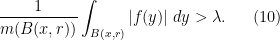
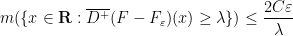
Lemma 25 (One-sided Hardy-Littlewood maximal inequality) Let
. Then
![\displaystyle m( \{ x \in {\bf R}: \sup_{h>0} \frac{1}{h} \int_{[x,x+h]} |f(t)|\ dt \geq \lambda \} ) \leq \frac{1}{\lambda} \int_{\bf R} |f(t)|\ dt.](https://s0.wp.com/latex.php?latex=%5Cdisplaystyle+m%28+%5C%7B+x+%5Cin+%7B%5Cbf+R%7D%3A+%5Csup_%7Bh%3E0%7D+%5Cfrac%7B1%7D%7Bh%7D+%5Cint_%7B%5Bx%2Cx%2Bh%5D%7D+%7Cf%28t%29%7C%5C+dt+%5Cgeq+%5Clambda+%5C%7D+%29+%5Cleq+%5Cfrac%7B1%7D%7B%5Clambda%7D+%5Cint_%7B%5Cbf+R%7D+%7Cf%28t%29%7C%5C+dt.&bg=ffffff&fg=000000&s=0&c=20201002)
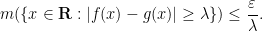
We will prove this lemma shortly, but let us first see how this, combined with the dense subclass result, will give the Lebesgue differentiation theorem. Let 


Applying the one-sided Hardy-Littlewood maximal inequality, we conclude that
![\displaystyle m( \{ x \in {\bf R}: \sup_{h>0} \frac{1}{h} \int_{[x,x+h]} |f(t)-g(t)|\ dt \geq \lambda \} ) \leq \frac{\varepsilon}{\lambda}.](https://s0.wp.com/latex.php?latex=%5Cdisplaystyle+m%28+%5C%7B+x+%5Cin+%7B%5Cbf+R%7D%3A+%5Csup_%7Bh%3E0%7D+%5Cfrac%7B1%7D%7Bh%7D+%5Cint_%7B%5Bx%2Cx%2Bh%5D%7D+%7Cf%28t%29-g%28t%29%7C%5C+dt+%5Cgeq+%5Clambda+%5C%7D+%29+%5Cleq+%5Cfrac%7B%5Cvarepsilon%7D%7B%5Clambda%7D.&bg=ffffff&fg=000000&s=0&c=20201002)
In a similar spirit, from Markov’s inequality we have
By subadditivity, we conclude that for all 
![\displaystyle \frac{1}{h} \int_{[x,x+h]} |f(t)-g(t)|\ dt < \lambda \ \ \ \ \ (5)](https://s0.wp.com/latex.php?latex=%5Cdisplaystyle+%5Cfrac%7B1%7D%7Bh%7D+%5Cint_%7B%5Bx%2Cx%2Bh%5D%7D+%7Cf%28t%29-g%28t%29%7C%5C+dt+%3C+%5Clambda+%5C+%5C+%5C+%5C+%5C+%285%29&bg=ffffff&fg=000000&s=0&c=20201002)

for all 
Now let 
![\displaystyle |\frac{1}{h} \int_{[x,x+h]} g(t)\ dt - g(x)| < \lambda](https://s0.wp.com/latex.php?latex=%5Cdisplaystyle+%7C%5Cfrac%7B1%7D%7Bh%7D+%5Cint_%7B%5Bx%2Cx%2Bh%5D%7D+g%28t%29%5C+dt+-+g%28x%29%7C+%3C+%5Clambda&bg=ffffff&fg=000000&s=0&c=20201002)
whenever
![\displaystyle |\frac{1}{h} \int_{[x,x+h]} f(t)\ dt - f(x)| < 3\lambda](https://s0.wp.com/latex.php?latex=%5Cdisplaystyle+%7C%5Cfrac%7B1%7D%7Bh%7D+%5Cint_%7B%5Bx%2Cx%2Bh%5D%7D+f%28t%29%5C+dt+-+f%28x%29%7C+%3C+3%5Clambda&bg=ffffff&fg=000000&s=0&c=20201002)
for all
![\displaystyle \limsup_{h \rightarrow 0} |\frac{1}{h} \int_{[x,x+h]} f(t)\ dt - f(x)| < 3\lambda](https://s0.wp.com/latex.php?latex=%5Cdisplaystyle+%5Climsup_%7Bh+%5Crightarrow+0%7D+%7C%5Cfrac%7B1%7D%7Bh%7D+%5Cint_%7B%5Bx%2Cx%2Bh%5D%7D+f%28t%29%5C+dt+-+f%28x%29%7C+%3C+3%5Clambda&bg=ffffff&fg=000000&s=0&c=20201002)
for all 
for almost every 

![\displaystyle \limsup_{h \rightarrow 0} |\frac{1}{h} \int_{[x,x+h]} f(t)\ dt - f(x)| = 0](https://s0.wp.com/latex.php?latex=%5Cdisplaystyle+%5Climsup_%7Bh+%5Crightarrow+0%7D+%7C%5Cfrac%7B1%7D%7Bh%7D+%5Cint_%7B%5Bx%2Cx%2Bh%5D%7D+f%28t%29%5C+dt+-+f%28x%29%7C+%3D+0&bg=ffffff&fg=000000&s=0&c=20201002)
for almost every
The only remaining task is to establish the one-sided Hardy-Littlewood maximal inequality. We will do so by using the rising sun lemma:
Lemma 26 (Rising sun lemma) Let
in
- For each
, either
, or else
and
.
- If
, then one must have
for all
.
Remark 27 To explain the name “rising sun lemma”, imagine the graph
of
(or rising from the east, if you will). Those
This lemma is proven using the following basic fact:
Exercise 28 Show that any open subset
of
Proof: (Proof of rising sun lemma) Let 


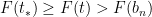
The second conclusion of the rising sun lemma is clear from construction, so it suffices to establish the first. Suppose first that 


Suppose for contradiction that there was 
![{A := \{ s \in [t,b]: F(s) \geq F(t)\}}](https://s0.wp.com/latex.php?latex=%7BA+%3A%3D+%5C%7B+s+%5Cin+%5Bt%2Cb%5D%3A+F%28s%29+%5Cgeq+F%28t%29%5C%7D%7D&bg=ffffff&fg=000000&s=0&c=20201002)


![{[b_n,b]}](https://s0.wp.com/latex.php?latex=%7B%5Bb_n%2Cb%5D%7D&bg=ffffff&fg=000000&s=0&c=20201002)

![{s \in [b_n,b]}](https://s0.wp.com/latex.php?latex=%7Bs+%5Cin+%5Bb_n%2Cb%5D%7D&bg=ffffff&fg=000000&s=0&c=20201002)


The case when
Now we can prove the one-sided Hardy-Littlewood maximal inequality. By upwards monotonicity, it will suffice to show that
![\displaystyle m( \{ x \in [a,b]: \sup_{h>0; [x,x+h] \subset [a,b]} \frac{1}{h} \int_{[x,x+h]} |f(t)|\ dt \geq \lambda \} ) \leq \frac{1}{\lambda} \int_{\bf R} |f(t)|\ dt](https://s0.wp.com/latex.php?latex=%5Cdisplaystyle+m%28+%5C%7B+x+%5Cin+%5Ba%2Cb%5D%3A+%5Csup_%7Bh%3E0%3B+%5Bx%2Cx%2Bh%5D+%5Csubset+%5Ba%2Cb%5D%7D+%5Cfrac%7B1%7D%7Bh%7D+%5Cint_%7B%5Bx%2Cx%2Bh%5D%7D+%7Cf%28t%29%7C%5C+dt+%5Cgeq+%5Clambda+%5C%7D+%29+%5Cleq+%5Cfrac%7B1%7D%7B%5Clambda%7D+%5Cint_%7B%5Cbf+R%7D+%7Cf%28t%29%7C%5C+dt&bg=ffffff&fg=000000&s=0&c=20201002)
for any compact interval
![\displaystyle m( \{ x \in [a,b]: \sup_{h>0; [x,x+h] \subset [a,b]} \frac{1}{h} \int_{[x,x+h]} |f(t)|\ dt > \lambda \} ) \leq \frac{1}{\lambda} \int_{\bf R} |f(t)|\ dt \ \ \ \ \ (7)](https://s0.wp.com/latex.php?latex=%5Cdisplaystyle+m%28+%5C%7B+x+%5Cin+%5Ba%2Cb%5D%3A+%5Csup_%7Bh%3E0%3B+%5Bx%2Cx%2Bh%5D+%5Csubset+%5Ba%2Cb%5D%7D+%5Cfrac%7B1%7D%7Bh%7D+%5Cint_%7B%5Bx%2Cx%2Bh%5D%7D+%7Cf%28t%29%7C%5C+dt+%3E+%5Clambda+%5C%7D+%29+%5Cleq+%5Cfrac%7B1%7D%7B%5Clambda%7D+%5Cint_%7B%5Cbf+R%7D+%7Cf%28t%29%7C%5C+dt+%5C+%5C+%5C+%5C+%5C+%287%29&bg=ffffff&fg=000000&s=0&c=20201002)
Fix
![\displaystyle F(x) := \int_{[a,x]} |f(t)|\ dt - (x-a) \lambda.](https://s0.wp.com/latex.php?latex=%5Cdisplaystyle+F%28x%29+%3A%3D+%5Cint_%7B%5Ba%2Cx%5D%7D+%7Cf%28t%29%7C%5C+dt+-+%28x-a%29+%5Clambda.&bg=ffffff&fg=000000&s=0&c=20201002)
By Lemma 16,
![\displaystyle \{ x \in (a,b]: \sup_{h>0; [x,x+h] \subset [a,b]} \frac{1}{h} \int_{[x,x+h]} |f(t)|\ dt > \lambda \} \subset \bigcup_n I_n,](https://s0.wp.com/latex.php?latex=%5Cdisplaystyle+%5C%7B+x+%5Cin+%28a%2Cb%5D%3A+%5Csup_%7Bh%3E0%3B+%5Bx%2Cx%2Bh%5D+%5Csubset+%5Ba%2Cb%5D%7D+%5Cfrac%7B1%7D%7Bh%7D+%5Cint_%7B%5Bx%2Cx%2Bh%5D%7D+%7Cf%28t%29%7C%5C+dt+%3E+%5Clambda+%5C%7D+%5Csubset+%5Cbigcup_n+I_n%2C&bg=ffffff&fg=000000&s=0&c=20201002)
since the property ![{\frac{1}{h} \int_{[x,x+h]} |f(t)|\ dt > \lambda}](https://s0.wp.com/latex.php?latex=%7B%5Cfrac%7B1%7D%7Bh%7D+%5Cint_%7B%5Bx%2Cx%2Bh%5D%7D+%7Cf%28t%29%7C%5C+dt+%3E+%5Clambda%7D&bg=ffffff&fg=000000&s=0&c=20201002)


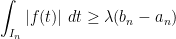
and thus
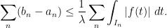
As the 
![\displaystyle \sum_n \int_{I_n} |f(t)|\ dt \leq \int_{[a,b]} |f(t)|\ dt,](https://s0.wp.com/latex.php?latex=%5Cdisplaystyle+%5Csum_n+%5Cint_%7BI_n%7D+%7Cf%28t%29%7C%5C+dt+%5Cleq+%5Cint_%7B%5Ba%2Cb%5D%7D+%7Cf%28t%29%7C%5C+dt%2C&bg=ffffff&fg=000000&s=0&c=20201002)
and the claim follows.
Exercise 29 (Two-sided Hardy-Littlewood maximal inequality) Let
where the supremum ranges over all intervals

Exercise 30 (Rising sun inequality) Let
be the one-sided signed Hardy-Littlewood maximal function
Establish the rising sun inequality
for all real
case, by invoking the rising sun lemma.) See these lecture notes for some further discussion of inequalities of this type, and applications to ergodic theory (and in particular the maximal ergodic theorem).
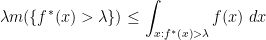
![\displaystyle f^*(x) := \sup_{h>0} \frac{1}{h} \int_{[x,x+h]} f(t)\ dt.](https://s0.wp.com/latex.php?latex=%5Cdisplaystyle+f%5E%2A%28x%29+%3A%3D+%5Csup_%7Bh%3E0%7D+%5Cfrac%7B1%7D%7Bh%7D+%5Cint_%7B%5Bx%2Cx%2Bh%5D%7D+f%28t%29%5C+dt.&bg=ffffff&fg=000000&s=0&c=20201002)
Exercise 31 Show that the left and right-hand sides in Exercise 30 are in fact equal when
. (Hint: one may first wish to try this in the case when
— 2. The Lebesgue differentiation theorem in higher dimensions —
Now we extend the Lebesgue differentiation theorem to higher dimensions. Theorem 15 does not have an obvious high-dimensional analogue, but Theorem 17 does:
Theorem 32 (Lebesgue differentiation theorem in high dimensions) Let
, one has
and
where
is the open ball of radius
centred at

From the triangle inequality we see that


so we see that the first conclusion of Theorem 32 implies the second. A point
Exercise 33 Call a function
- Show that
for all
.
- Show that Theorem 32 implies a generalisation of itself in which the condition of absolute integrability of
Exercise 34 For each
be a subset of
with the property that
for some
To prove Theorem 32, we use the density argument. The dense subclass case is easy:
Exercise 35 Show that Theorem 32 holds whenever
The quantitative estimate needed is the following:
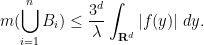
Theorem 36 (Hardy-Littlewood maximal inequality) Let
for some constant
depending only on
.

Remark 37 The expression
is known as the Hardy-Littlewood maximal function of
. It is an important function in the field of (real-variable) harmonic analysis.
Exercise 38 Use the density argument to show that Theorem 36 implies Theorem 32.
In the one-dimensional case, this estimate was established via the rising sun lemma. Unfortunately, that lemma relied heavily on the ordered nature of 


Lemma 39 (Vitali-type covering lemma) Let
be a finite collection of open balls in
of disjoint balls in this collection, such that
In particular, by finite subadditivity,

Proof: We use a greedy algorithm argument, selecting the balls 
- Step 0. Initialise
(so that, initially, there are no balls
- Step 1. Look at all the balls
that do not already intersect one of the
- Step 2. Locate the largest ball
and then incrementing
to
. Then return to Step 1.
Note that at each iteration of this algorithm, the number of available balls amongst the 

For this, we argue as follows. Take any ball 


Exercise 40 Technically speaking, the above algorithmic argument was not phrased in the standard language of formal mathematical deduction, because in that language, any mathematical object (such as the natural number
of balls that represent the outcome of the above algorithm after
). For this particular algorithm, there are also more ad hoc approaches that exploit the relatively simple nature of the algorithm to allow for a less notationally complicated construction.) More generally, it is possible to use this time parameter trick to convert any construction involving a provably terminating algorithm into a construction that does not redefine any variable. (It is however dangerous to work with any algorithm that has an infinite run time, unless one has a suitably strong convergence result for the algorithm that allows one to take limits, either in the classical sense or in the more general sense of jumping to limit ordinals; in the latter case, one needs to use transfinite induction in order to ensure that the use of such algorithms is rigorous.)
Remark 41 The actual Vitali covering lemma is slightly different to this one, as the linked Wikipedia page shows. Actually there is a family of related covering lemmas which are useful for a variety of tasks in harmonic analysis, see for instance this book by de Guzmán for further discussion.
Now we can prove the Hardy-Littlewood inequality, which we will do with the constant 

as the non-strict case then follows by perturbing
Fix
whenever 

By construction, for every 

By compactness of
By (10), on each ball

summing in 
Since the
Exercise 42 Improve the constant
in the Hardy-Littlewood maximal inequality to
. (Hint: observe that with the construction used to prove the Vitali covering lemma, the centres of the balls
and not just in
. To exploit this observation one may need to first create an epsilon of room, as the centers are not by themselves sufficient to cover the required set.)
Remark 43 The optimal value of
is not known in general, although a fairly recent result of Melas gives the surprising conclusion that the optimal value of
is
. It is known that
. See this blog post for some further discussion.
Exercise 44 (Dyadic maximal inequality) If
where the supremum ranges over all dyadic cubes
that contain

Exercise 45 (Besicovitch covering lemma in one dimension) Let
be a finite family of open intervals in
of intervals such that
; and
- Each point
.
(Hint: First refine the family of intervals so that no interval
is contained in the union of the the other intervals. At that point, show that it is no longer possible for a point to be contained in three of the intervals.) There is a variant of this lemma that holds in higher dimensions, known as the Besicovitch covering lemma.
Exercise 46 Let
be a Borel measure (i.e. a countably additive measure on the Borel
-algebra) on
for every interval
for every Borel measurable set
for any absolutely integrable function
, where the supremum ranges over all open intervals

Exercise 47 (Cousin’s theorem) Prove Cousin’s theorem: given any function
on a compact interval
, together with real numbers
. (Hint: use the Heine-Borel theorem, which asserts that any open cover of
Now we turn to consequences of the Lebesgue differentiation theorem. Given a Lebesgue measurable set 

![{E = [-1,1] \backslash \{0\}}](https://s0.wp.com/latex.php?latex=%7BE+%3D+%5B-1%2C1%5D+%5Cbackslash+%5C%7B0%5C%7D%7D&bg=ffffff&fg=000000&s=0&c=20201002)


Exercise 48 If
Exercise 49 Let
- Using Exercise 34 and Exercise 48, show that there exists a cube
of positive sidelength such that
.
- Give an alternate proof of the above claim that avoids the Lebesgue differentiation theorem. (Hint: reduce to the case when
- Use the above result to give an alternate proof of the Steinhaus theorem (Exercise 22).
Of course, one can replace cubes here by other comparable shapes, such as balls. (Indeed, a good principle to adopt in analysis is that cubes and balls are “equivalent up to constants”, in that a cube of some sidelength can be contained in a ball of comparable radius, and vice versa. This type of mental equivalence is analogous to, though not identical with, the famous dictum that a topologist cannot distinguish a doughnut from a coffee cup.)
Exercise 50
- Give an example of a compact set
of positive measure such that
for every interval
.)
- Give an example of a measurable set
such that
for every interval
. The complement of the set
Exercise 51 (Approximations to the identity) Define a good kernel to be a measurable function
which is non-negative, radial (which means that there is a function
such that
), radially non-increasing (so that
is a non-increasing function), and has total mass
equal to
for
are then said to be a good family of approximations to the identity.
- Show that the heat kernels
and Poisson kernels
are good families of approximations to the identity, if the constant
is chosen correctly (in fact one has
, but you are not required to establish this). (Note that we have modified the usual formulation of the heat kernel by replacing
in order to make it conform to the notational conventions used in this exercise.)
- Show that if
is a good kernel, then
for some constants
depending only on
.)
- Establish the quantitative upper bound
for any absolutely integrable function
depending only on
- Show that if
converges to
. (Hint: split
as the sum of
.) In particular,
converges pointwise almost everywhere to


— 3. Almost everywhere differentiability —
As we see in undergraduate real analysis, not every continuous function 

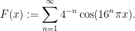
Exercise 52 (Weierstrass function) Let
be the function
- Show that
- Show that for every interval
with
and
for some absolute constant
- Show that
The difficulty here is that a continuous function can still contain a large amount of oscillation, which can lead to breakdown of differentiability. However, if one can somehow limit the amount of oscillation present, then one can often recover a fair bit of differentiability. For instance, we have
Theorem 53 (Monotone differentiation theorem) Any function
Exercise 54 Show that every monotone function is measurable.
To prove this theorem, we just treat the case when
We also first focus on the case when
- The upper right derivative
;
- The lower right derivative
;
- The upper left derivative
;
- The lower right derivative
.
Regardless of whether ![{[-\infty,\infty]}](https://s0.wp.com/latex.php?latex=%7B%5B-%5Cinfty%2C%5Cinfty%5D%7D&bg=ffffff&fg=000000&s=0&c=20201002)
Exercise 55 If
A function

We also have the trivial inequalities

If

The one-sided Hardy-Littlewood maximal inequality has an analogue in this setting:
Lemma 56 (One-sided Hardy-Littlewood inequality) Let
Similarly for the other three Dini derivatives of
If
for some absolute constant
.
![\displaystyle m( \{ x \in [a,b]: \overline{D^+} F(x) \geq \lambda \} ) \leq \frac{F(b)-F(a)}{\lambda}.](https://s0.wp.com/latex.php?latex=%5Cdisplaystyle+m%28+%5C%7B+x+%5Cin+%5Ba%2Cb%5D%3A+%5Coverline%7BD%5E%2B%7D+F%28x%29+%5Cgeq+%5Clambda+%5C%7D+%29+%5Cleq+%5Cfrac%7BF%28b%29-F%28a%29%7D%7B%5Clambda%7D.&bg=ffffff&fg=000000&s=0&c=20201002)
![\displaystyle m( \{ x \in [a,b]: \overline{D^+} F(x) \geq \lambda \} ) \leq C\frac{F(b)-F(a)}{\lambda}](https://s0.wp.com/latex.php?latex=%5Cdisplaystyle+m%28+%5C%7B+x+%5Cin+%5Ba%2Cb%5D%3A+%5Coverline%7BD%5E%2B%7D+F%28x%29+%5Cgeq+%5Clambda+%5C%7D+%29+%5Cleq+C%5Cfrac%7BF%28b%29-F%28a%29%7D%7B%5Clambda%7D&bg=ffffff&fg=000000&s=0&c=20201002)
Remark 57 Note that if one naively applies the fundamental theorems of calculus, one can formally see that the first part of Lemma 56 is equivalent to Lemma 25. We cannot however use this argument rigorously because we have not established the necessary fundamental theorems of calculus to do this. Nevertheless, we can borrow the proof of Lemma 25 without difficulty to use here, and this is exactly what we will do.
Proof: We just prove the continuous case and leave the discontinuous case as an exercise.
It suffices to prove the claim for 

![{[-b,-a]}](https://s0.wp.com/latex.php?latex=%7B%5B-b%2C-a%5D%7D&bg=ffffff&fg=000000&s=0&c=20201002)


We may apply the rising sun lemma (Lemma 26) to the continuous function 


Observe that if 


But we can rearrange the inequality 


The discontinuous case is left as an exercise.
Exercise 58 Prove Lemma 56 in the discontinuous case. (Hint: the rising sun lemma is no longer available, but one can use either the Vitali-type covering lemma (which will give
) or the Besicovitch lemma (which will give
), by modifying the proof of Theorem 36.
Sending 


is a null set, since by letting 


Clearly
Lemma 59 (
.
Indeed, this lemma implies that
Proof: We begin by applying the rising sun lemma to the function 


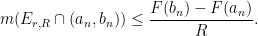
But we can rearrange the inequality 
![\displaystyle m( E_{r,R} \cap [a,b] ) \leq \frac{r}{R} \sum_n b_n - a_n.](https://s0.wp.com/latex.php?latex=%5Cdisplaystyle+m%28+E_%7Br%2CR%7D+%5Ccap+%5Ba%2Cb%5D+%29+%5Cleq+%5Cfrac%7Br%7D%7BR%7D+%5Csum_n+b_n+-+a_n.&bg=ffffff&fg=000000&s=0&c=20201002)
But the 
Remark 60 Note if
here from the second part of Lemma 56, and one would then be unable to prevent
This concludes the proof of Theorem 53 in the continuous monotone non-decreasing case. Now we work on removing the continuity hypothesis (which was needed in order to make the rising sun lemma work properly). If we naively try to run the density argument as we did in previous sections, then (for once) the argument does not work very well, as the space of continuous monotone functions are not sufficiently dense in the space of all monotone functions in the relevant sense (which, in this case, is in the total variation sense, which is what is needed to invoke such tools as Lemma 56.). To bridge this gap, we have to supplement the continuous monotone functions with another class of monotone functions, known as the jump functions.
Definition 61 (Jump function) A basic jump function
is a function of the form
for some real numbers
and
; we call
the point of discontinuity for
the fraction. Observe that such functions are monotone non-decreasing, but have a discontinuity at one point. A jump function is any absolutely convergent combination of basic jump functions, i.e. a function of the form
, where
is a basic jump function, and the
are positivereals with
. If there are only finitely many
Thus, for instance, if 
Clearly, all jump functions are monotone non-decreasing. From the absolute convergence of the 


The key fact is that these functions, together with the continuous monotone functions, essentially generate all monotone functions, at least in the bounded case:
Lemma 62 (Continuous-singular decomposition for monotone functions) Let
- The only discontinuities of
and
both exist, but are unequal, with
.
- There are at most countably many discontinuities of
- If
and a jump function
.
Remark 63 This decomposition is part of the more general Lebesgue decomposition, which we will discuss later in this course.
Proof: By monotonicity, the limits 
By 1., whenever there is a discontinuity 


Now we prove 3. Let 

![{\theta_x := \frac{F(x)-F_-(x)}{F_+(x)-F_-(x)} \in [0,1]}](https://s0.wp.com/latex.php?latex=%7B%5Ctheta_x+%3A%3D+%5Cfrac%7BF%28x%29-F_-%28x%29%7D%7BF_%2B%28x%29-F_-%28x%29%7D+%5Cin+%5B0%2C1%5D%7D&bg=ffffff&fg=000000&s=0&c=20201002)

Note that 


is a jump function.
As discussed previously,

where 


for all 
![{\sum_{x \in A \cap [a,b]} c_x}](https://s0.wp.com/latex.php?latex=%7B%5Csum_%7Bx+%5Cin+A+%5Ccap+%5Ba%2Cb%5D%7D+c_x%7D&bg=ffffff&fg=000000&s=0&c=20201002)

![{x \in A \cap [a,b]}](https://s0.wp.com/latex.php?latex=%7Bx+%5Cin+A+%5Ccap+%5Ba%2Cb%5D%7D&bg=ffffff&fg=000000&s=0&c=20201002)

Exercise 64 Show that the decomposition of a bounded monotone non-decreasing function
Exercise 65 Find a suitable generalisation of the notion of a jump function that allows one to extend the above decomposition to unbounded monotone functions, and then prove this extension. (Hint: the notion to shoot for here is that of a “locally jump function”.)
Now we can finish the proof of Theorem 53. As noted previously, it suffices to prove the claim for monotone non-decreasing functions. As differentiability is a local condition, we can easily reduce to the case of bounded monotone non-decreasing functions, since to test differentiability of a monotone non-decreasing function 

Now, finally, we are able to use the density argument, using the piecewise constant jump functions as the dense subclass, and using the second part of Lemma 56 for the quantitative estimate; fortunately for us, the density argument does not particularly care that there is a loss of a constant factor in this estimate.
For piecewise constant jump functions, the claim is clear (indeed, the derivative exists and is zero outside of finitely many discontinuities). Now we run the density argument. Let 


for some absolute constant 


Just as the integration theory of unsigned functions can be used to develop the integration theory of the absolutely convergent functions (see Notes 2), the differentiation theory of monotone functions can be used to develop a parallel differentiation theory for the class of functions of bounded variation:
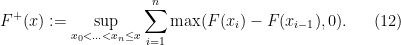
Definition 66 (Bounded variation) Let
(or
for short) of
where the supremum ranges over all finite increasing sequences
of real numbers with
; this is a quantity in
. We say that
or just
.)
Given any intervalof
thus the definition is the same, but the points
. We say that a function
is finite.

![\displaystyle \|F\|_{TV([a,b])} := \sup_{a \leq x_0 < \ldots < x_n \leq b} \sum_{i=1}^n |F(x_i) - F(x_{i-1})|;](https://s0.wp.com/latex.php?latex=%5Cdisplaystyle+%5C%7CF%5C%7C_%7BTV%28%5Ba%2Cb%5D%29%7D+%3A%3D+%5Csup_%7Ba+%5Cleq+x_0+%3C+%5Cldots+%3C+x_n+%5Cleq+b%7D+%5Csum_%7Bi%3D1%7D%5En+%7CF%28x_i%29+-+F%28x_%7Bi-1%7D%29%7C%3B&bg=ffffff&fg=000000&s=0&c=20201002)
Exercise 67 If
for any interval
Exercise 68 For any functions
, establish the triangle property
and the homogeneity property
for any
. Also show that
if and only if
Exercise 69 If
whenever
.
Exercise 70
- Show that every function
and
, are well-defined.
- Give a counterexample of a bounded, continuous, compactly supported function
Exercise 71 Let
. Show that
. (Hint: the upper bound
is relatively easy to establish. To obtain the lower bound, use the density argument.)
Much as an absolutely integrable function can be expressed as the difference of its positive and negative parts, a bounded variation function can be expressed as the difference of two bounded monotone functions:
Proposition 72 A function
Proof: It is clear from Exercises 67, 68 that the difference of two bounded monotone functions is bounded. Now define the positive variation 
It is clear from construction that this is a monotone increasing function, taking values between 


If 


Exercise 73 Let
by
Establish the identities
and
for every interval
,
, and
. (Hint: The main difficulty comes from the fact that a partition
that is good for

![\displaystyle \|F\|_{TV[a,b]} = F^+(b)-F^+(a) + F^-(b)-F^-(a),](https://s0.wp.com/latex.php?latex=%5Cdisplaystyle+%5C%7CF%5C%7C_%7BTV%5Ba%2Cb%5D%7D+%3D+F%5E%2B%28b%29-F%5E%2B%28a%29+%2B+F%5E-%28b%29-F%5E-%28a%29%2C&bg=ffffff&fg=000000&s=0&c=20201002)

From Proposition 72 and Theorem 53 we immediately obtain
Corollary 74 (BV differentiation theorem) Every bounded variation function is differentiable almost everywhere.
Exercise 75 Call a function locally of bounded variation if it is of bounded variation on every compact interval
Exercise 76 (Lipschitz differentiation theorem, one-dimensional case) A function
such that
for all
; the smallest
Remark 77 The same result is true in higher dimensions, and is known as the Radamacher differentiation theorem, but we will defer the proof of this theorem to subsequent notes, when we have the powerful tool of the Fubini-Tonelli theorem available, that is particularly useful for deducing higher-dimensional results in analysis from lower-dimensional ones.
Exercise 78 A function
for all
and
. Show that if
is equal almost everywhere to a monotone non-decreasing function, and so is itself almost everywhere differentiable. (Hint: Drawing the graph of
— 4. The second fundamental theorem of calculus —
We are now finally ready to attack the second fundamental theorem of calculus in the cases where
One half of the second fundamental theorem is easy:
Proposition 79 (Upper bound for second fundamental theorem) Let
In particular,
![\displaystyle \int_{[a,b]} F'(x)\ dx \leq F(b)-F(a).](https://s0.wp.com/latex.php?latex=%5Cdisplaystyle+%5Cint_%7B%5Ba%2Cb%5D%7D+F%27%28x%29%5C+dx+%5Cleq+F%28b%29-F%28a%29.&bg=ffffff&fg=000000&s=0&c=20201002)
Proof: It is convenient to extend 


converge pointwise almost everywhere to
![\displaystyle \int_{[a,b]} F'(x)\ dx \leq \liminf_{n \rightarrow \infty} \int_{[a,b]} \frac{F(x+1/n) - F(x)}{1/n}\ dx.](https://s0.wp.com/latex.php?latex=%5Cdisplaystyle+%5Cint_%7B%5Ba%2Cb%5D%7D+F%27%28x%29%5C+dx+%5Cleq+%5Climinf_%7Bn+%5Crightarrow+%5Cinfty%7D+%5Cint_%7B%5Ba%2Cb%5D%7D+%5Cfrac%7BF%28x%2B1%2Fn%29+-+F%28x%29%7D%7B1%2Fn%7D%5C+dx.&bg=ffffff&fg=000000&s=0&c=20201002)
The right-hand side can be rearranged as
![\displaystyle \liminf_{n \rightarrow \infty} n (\int_{[a+1/n,b+1/n]} F(y)\ dy - \int_{[a,b]} F(x)\ dx)](https://s0.wp.com/latex.php?latex=%5Cdisplaystyle+%5Climinf_%7Bn+%5Crightarrow+%5Cinfty%7D+n+%28%5Cint_%7B%5Ba%2B1%2Fn%2Cb%2B1%2Fn%5D%7D+F%28y%29%5C+dy+-+%5Cint_%7B%5Ba%2Cb%5D%7D+F%28x%29%5C+dx%29&bg=ffffff&fg=000000&s=0&c=20201002)
which can be rearranged further as
![\displaystyle \liminf_{n \rightarrow \infty} n (\int_{[b,b+1/n]} F(x)\ dx - \int_{[a,a+1/n]} F(x)\ dx).](https://s0.wp.com/latex.php?latex=%5Cdisplaystyle+%5Climinf_%7Bn+%5Crightarrow+%5Cinfty%7D+n+%28%5Cint_%7B%5Bb%2Cb%2B1%2Fn%5D%7D+F%28x%29%5C+dx+-+%5Cint_%7B%5Ba%2Ca%2B1%2Fn%5D%7D+F%28x%29%5C+dx%29.&bg=ffffff&fg=000000&s=0&c=20201002)
Since 


and the claim follows.
Exercise 80 Show that any function of bounded variation has an (almost everywhere defined) derivative that is absolutely integrable.
In the Lipschitz case, one can do better:
Exercise 81 (Second fundamental theorem for Lipschitz functions) Let
. (Hint: Argue as in the proof of Proposition 79, but use the dominated convergence theorem in place of Fatou’s lemma.)
Exercise 82 (Integration by parts formula) Let
be Lipschitz continuous functions. Show that
(Hint: first show that the product of two Lipschitz continuous functions on
![\displaystyle \int_{[a,b]} F'(x) G(x)\ dx = F(b) G(b)-F(a) G(a)](https://s0.wp.com/latex.php?latex=%5Cdisplaystyle+%5Cint_%7B%5Ba%2Cb%5D%7D+F%27%28x%29+G%28x%29%5C+dx+%3D+F%28b%29+G%28b%29-F%28a%29+G%28a%29+&bg=ffffff&fg=000000&s=0&c=20201002)
![\displaystyle - \int_{[a,b]} F(x) G'(x)\ dx.](https://s0.wp.com/latex.php?latex=%5Cdisplaystyle+-+%5Cint_%7B%5Ba%2Cb%5D%7D+F%28x%29+G%27%28x%29%5C+dx.&bg=ffffff&fg=000000&s=0&c=20201002)
Now we return to the monotone case. Inspired by the Lipschitz case, one may hope to recover equality in Proposition 79 for such functions 
![{\int_{[a,b]} F'(x)\ dx}](https://s0.wp.com/latex.php?latex=%7B%5Cint_%7B%5Ba%2Cb%5D%7D+F%27%28x%29%5C+dx%7D&bg=ffffff&fg=000000&s=0&c=20201002)
Exercise 83 Show that if
One may hope that jump functions – in which all the fluctuation is concentrated in a countable set – are the only obstruction to the second fundamental theorem of calculus holding for monotone functions, and that as long as one restricts attention to continuous monotone functions, that one can recover the second fundamental theorem. However, this is still not true, because it is possible for all the fluctuation to now be concentrated, not in a countable collection of jump discontinuities, but instead in an uncountable set of zero measure, such as the middle thirds Cantor set (Exercise 10 from Notes 1). This can be illustrated by the key counterexample of the Cantor function, also known as the Devil’s staircase function. The construction of this function is detailed in the exercise below.
Exercise 84 (Cantor function) Define the functions
recursively as follows:
- Set
for all
.
- For each
- Graph
,
,
, and
(preferably on a single graph).
- Show that for each
,
is a continuous monotone non-decreasing function with
and
. (Hint: induct on
- Show that for each
for each
. This limit is known as the Cantor function.
- Show that the Cantor function
and
.
- Show that if
, so that the second fundamental theorem of calculus fails for this function.
- Show that
for any digits
. Thus the Cantor function, in some sense, converts base three expansions to base two expansions.
- Let
be one of the intervals used in the
cover
. Show that
, but
is an interval of length
.
- Show that
![\displaystyle F_n(x) := \left\{ \begin{array}{ll} \frac{1}{2} F_{n-1}(3x) & \hbox{ if } x \in [0,1/3]; \\ \frac{1}{2} & \hbox{ if } x \in (1/3,2/3); \\ \frac{1}{2} + \frac{1}{2} F_{n-1}(3x-2) & \hbox{ if } x \in [2/3,1] \end{array} \right.](https://s0.wp.com/latex.php?latex=%5Cdisplaystyle+F_n%28x%29+%3A%3D+%5Cleft%5C%7B+%5Cbegin%7Barray%7D%7Bll%7D+%5Cfrac%7B1%7D%7B2%7D+F_%7Bn-1%7D%283x%29+%26+%5Chbox%7B+if+%7D+x+%5Cin+%5B0%2C1%2F3%5D%3B+%5C%5C+%5Cfrac%7B1%7D%7B2%7D+%26+%5Chbox%7B+if+%7D+x+%5Cin+%281%2F3%2C2%2F3%29%3B+%5C%5C+%5Cfrac%7B1%7D%7B2%7D+%2B+%5Cfrac%7B1%7D%7B2%7D+F_%7Bn-1%7D%283x-2%29+%26+%5Chbox%7B+if+%7D+x+%5Cin+%5B2%2F3%2C1%5D+%5Cend%7Barray%7D+%5Cright.+&bg=ffffff&fg=000000&s=0&c=20201002)
Remark 85 This example shows that the classical derivative
of a function has some defects; it cannot “see” some of the variation of a continuous monotone function such as the Cantor function. Much later in this series, we will rectify this by introducing the concept of the weak derivative of a function, which despite the name, is more able than the strong derivative to detect this type of singular variation behaviour. (We will also encounter the Riemann-Stieltjes integral in later notes, which is another (closely related) way to capture all of the variation of a monotone function, and which is related to the classical derivative via the Lebesgue-Radon-Nikodym theorem.)
In view of this counterexample, we see that we need to add an additional hypothesis to the continuous monotone non-increasing function
- A function
whenever
- A function
Definition 86 A function
whenever
is a finite collection of disjoint intervals of total length
at most
We define absolute continuity for a functionare of course now required to lie in the domain
The following exercise places absolute continuity in relation to other regularity properties:
- Show that every absolutely continuous function is uniformly continuous and therefore continuous.
- Show that every absolutely continuous function is of bounded variation on every compact interval
- Show that every Lipschitz continuous function is absolutely continuous.
- Show that the function
is absolutely continuous, but not Lipschitz continuous, on the interval
- Show that the Cantor function from Exercise 84 is continuous, monotone, and uniformly continuous, but not absolutely continuous, on
- If
is absolutely continuous, and that
- Show that the sum or product of two absolutely continuous functions on an interval
Exercise 88
- Show that absolutely continuous functions map null sets to null sets, i.e. if
is absolutely continuous and
is also a null set.
- Show that the Cantor function does not have this property.
For absolutely continuous functions, we can recover the second fundamental theorem of calculus:
Theorem 89 (Second fundamental theorem for absolutely continuous functions) Let
Proof: Our main tool here will be Cousin’s theorem (Exercise 47).
By Exercise 80, 
![{U \subset [a,b]}](https://s0.wp.com/latex.php?latex=%7BU+%5Csubset+%5Ba%2Cb%5D%7D&bg=ffffff&fg=000000&s=0&c=20201002)

Let ![{E \subset [a,b]}](https://s0.wp.com/latex.php?latex=%7BE+%5Csubset+%5Ba%2Cb%5D%7D&bg=ffffff&fg=000000&s=0&c=20201002)

Now define a gauge function
- If
, we define
to be small enough that the open interval
lies in
- If
, then
holds whenever
, and such that
whenever
; such a
and
.
Applying Cousin’s theorem, we can find a partition
We can express

To estimate the size of this sum, let us first consider those 

and thus
Next, we consider those 

and

and thus

On the other hand, from construction again we have
![\displaystyle \int_{[t_{j-1},t_j]} F'(y)\ dy = (t_j -t_{j-1}) F'(t^*_j) + O(\varepsilon |t_j - t_{j-1}| )](https://s0.wp.com/latex.php?latex=%5Cdisplaystyle+%5Cint_%7B%5Bt_%7Bj-1%7D%2Ct_j%5D%7D+F%27%28y%29%5C+dy+%3D+%28t_j+-t_%7Bj-1%7D%29+F%27%28t%5E%2A_j%29+%2B+O%28%5Cvarepsilon+%7Ct_j+-+t_%7Bj-1%7D%7C+%29&bg=ffffff&fg=000000&s=0&c=20201002)
and thus
![\displaystyle F(t_j) - F(t_{j-1}) = \int_{[t_{j-1},t_j]} F'(y)\ dy + O(\varepsilon |t_j - t_{j-1}| ).](https://s0.wp.com/latex.php?latex=%5Cdisplaystyle+F%28t_j%29+-+F%28t_%7Bj-1%7D%29+%3D+%5Cint_%7B%5Bt_%7Bj-1%7D%2Ct_j%5D%7D+F%27%28y%29%5C+dy+%2B+O%28%5Cvarepsilon+%7Ct_j+-+t_%7Bj-1%7D%7C+%29.&bg=ffffff&fg=000000&s=0&c=20201002)
Summing in

where 
![{[t_{j-1},t_j]}](https://s0.wp.com/latex.php?latex=%7B%5Bt_%7Bj-1%7D%2Ct_j%5D%7D&bg=ffffff&fg=000000&s=0&c=20201002)
![{[a,b] \backslash U}](https://s0.wp.com/latex.php?latex=%7B%5Ba%2Cb%5D+%5Cbackslash+U%7D&bg=ffffff&fg=000000&s=0&c=20201002)
![\displaystyle \int_{S} F'(y)\ dy = \int_{[a,b]} F'(y)\ dy + O(\varepsilon).](https://s0.wp.com/latex.php?latex=%5Cdisplaystyle+%5Cint_%7BS%7D+F%27%28y%29%5C+dy+%3D+%5Cint_%7B%5Ba%2Cb%5D%7D+F%27%28y%29%5C+dy+%2B+O%28%5Cvarepsilon%29.&bg=ffffff&fg=000000&s=0&c=20201002)
Putting everything together, we conclude that
![\displaystyle F(b)-F(a) = \int_{[a,b]} F'(y)\ dy + O(\varepsilon) + O( \varepsilon |b-a| ).](https://s0.wp.com/latex.php?latex=%5Cdisplaystyle+F%28b%29-F%28a%29+%3D+%5Cint_%7B%5Ba%2Cb%5D%7D+F%27%28y%29%5C+dy+%2B+O%28%5Cvarepsilon%29+%2B+O%28+%5Cvarepsilon+%7Cb-a%7C+%29.&bg=ffffff&fg=000000&s=0&c=20201002)
Since
Combining this result with Exercise 87, we obtain a satisfactory classification of the absolutely continuous functions:
Exercise 90 Show that a function
for some absolutely integrable
and a constant
Exercise 91 (Compatibility of the strong and weak derivatives in the absolutely continuous case) Let
be a continuously differentiable function supported in a compact subset of
.
Inspecting the proof of Theorem 89, we see that the absolute continuity was used primarily in two ways: firstly, to ensure the almost everywhere existence, and to control an exceptional null set
Proposition 92 (Second fundamental theorem of calculus, again) Let
Proof: This will be similar to the proof of Theorem 89, the one main new twist being that we need several open sets 

For every natural number 


Now define a gauge function
- If
, and also small enough that
exists and is finite here.)
- If
Applying Cousin’s theorem, we can find a partition
As before, we express
For the contributions of those
where
![\displaystyle \int_{[a,b] \backslash S} |F'(x)|\ dx \leq \int_{\bigcup_{m=1}^\infty U_m} |F'(x)|\ dx \leq \varepsilon](https://s0.wp.com/latex.php?latex=%5Cdisplaystyle+%5Cint_%7B%5Ba%2Cb%5D+%5Cbackslash+S%7D+%7CF%27%28x%29%7C%5C+dx+%5Cleq+%5Cint_%7B%5Cbigcup_%7Bm%3D1%7D%5E%5Cinfty+U_m%7D+%7CF%27%28x%29%7C%5C+dx+%5Cleq+%5Cvarepsilon&bg=ffffff&fg=000000&s=0&c=20201002)
we thus have
Now we turn to those

fir these intervals, and so

Next, for each 
![{[t_{j-1},t_j] \subset U_m}](https://s0.wp.com/latex.php?latex=%7B%5Bt_%7Bj-1%7D%2Ct_j%5D+%5Csubset+U_m%7D&bg=ffffff&fg=000000&s=0&c=20201002)

Putting all this together, we again have
Since
Remark 93 The above proposition is yet another illustration of how the property of everywhere differentiability is significantly better than that of almost everywhere differentiability. In practice, though, the above proposition is not as useful as one might initially think, because there are very few methods that establish the everywhere differentiability of a function that do not also establish continuous differentiability (or at least Riemann integrability of the derivative), at which point one could just use Theorem 11 instead.
Exercise 94 Let
be the function defined by setting
when
. Show that
Exercise 95 (Henstock-Kurzweil integral) Let
if for every
whenever
are such that
for every
the Henstock-Kurzweil integral of
.
- Show that if a function is Henstock-Kurzweil integrable, it has a unique Henstock-Kurzweil integral. (Hint: use Cousin’s theorem.)
- Show that if a function is Riemann integrable, then it is Henstock-Kurzweil integrable, and the Henstock-Kurzweil integral
.
- Show that if a function
- Show that if
- Explain why the above results give an alternate proof of Exercise 10 and of Proposition 92.

Remark 96 As the above exercise indicates, the Henstock-Kurzweil integral (also known as the Denjoy integral or Perron integral) extends the Riemann integral and the absolutely convergent Lebesgue integral, at least as long as one restricts attention to functions that are defined and are finite everywhere (in contrast to the Lebesgue integral, which is willing to tolerate functions being infinite or undefined so long as this only occurs on a null set). It is the notion of integration that is most naturally associated with the fundamental theorem of calculus for everywhere differentiable functions, as seen in part 4 of the above exercise; it can also be used as a unified framework for all the proofs in this section that invoked Cousin’s theorem. The Henstock-Kurzweil integral can also integrate some (highly oscillatory) functions that the Lebesgue integral cannot, such as the derivative
can sum conditionally convergent series
, even if they are not absolutely integrable. However, much as conditional summation is not always well-behaved with respect to rearrangement, the Henstock-Kurzweil integral does not always react well to changes of variable; also, due to its reliance on the order structure of the real line

197 comments
Comments feed for this article
4 March, 2016 at 11:56 am
Anonymous
In Theorem 24, do we have that the converse is actually also true, namely, if the identity
![\displaystyle \int_{[a,b]}F'(x)\ dx=F(b)-F(a)](https://s0.wp.com/latex.php?latex=%5Cdisplaystyle+%5Cint_%7B%5Ba%2Cb%5D%7DF%27%28x%29%5C+dx%3DF%28b%29-F%28a%29&bg=ffffff&fg=545454&s=0&c=20201002) makes sense, then
makes sense, then  must be absolutely continuous on
 ![[a,b]](https://s0.wp.com/latex.php?latex=%5Ba%2Cb%5D&bg=ffffff&fg=545454&s=0&c=20201002) ?
?
If![F:[a,b]\to\mathbb{R}](https://s0.wp.com/latex.php?latex=F%3A%5Ba%2Cb%5D%5Cto%5Cmathbb%7BR%7D&bg=ffffff&fg=545454&s=0&c=20201002) is differentiable, can we conclude that
is differentiable, can we conclude that  is absolutely continuous on
 ![[a,b]](https://s0.wp.com/latex.php?latex=%5Ba%2Cb%5D&bg=ffffff&fg=545454&s=0&c=20201002) so that Proposition 25 is implied by Theorem 24?
so that Proposition 25 is implied by Theorem 24?
4 March, 2016 at 3:41 pm
Terence Tao
Theorem 6 serves as a converse to Theorem 24. Note that just having well-defined and absolutely integrable and
 ![\int_{[a,b]} F'(x)\ dx = F(b)-F(a)](https://s0.wp.com/latex.php?latex=%5Cint_%7B%5Ba%2Cb%5D%7D+F%27%28x%29%5C+dx+%3D+F%28b%29-F%28a%29&bg=ffffff&fg=545454&s=0&c=20201002) for a single choice of
for a single choice of  is not sufficient (take for instance
  to be the Cantor function from Exercise 47, but with
  set equal to 0 rather than 1).
Incidentally, all of these questions are great exercises to work out yourself; see https://terrytao.wordpress.com/career-advice/ask-yourself-dumb-questions-%E2%80%93-and-answer-them/
4 March, 2016 at 8:48 pm
Anonymous
Suppose![F:[a,b]\to\mathbb{R}](https://s0.wp.com/latex.php?latex=F%3A%5Ba%2Cb%5D%5Cto%5Cmathbb%7BR%7D&bg=ffffff&fg=545454&s=0&c=20201002) is differentiable. It is true that
is differentiable. It is true that
![\displaystyle \int_{[a,b]}F'(x)\ dx=F(b)-F(a)](https://s0.wp.com/latex.php?latex=%5Cdisplaystyle+%5Cint_%7B%5Ba%2Cb%5D%7DF%27%28x%29%5C+dx%3DF%28b%29-F%28a%29&bg=ffffff&fg=545454&s=0&c=20201002)
![\displaystyle \int_{[a,x]}F'(x)\ dx=F(x)-F(a)](https://s0.wp.com/latex.php?latex=%5Cdisplaystyle+%5Cint_%7B%5Ba%2Cx%5D%7DF%27%28x%29%5C+dx%3DF%28x%29-F%28a%29&bg=ffffff&fg=545454&s=0&c=20201002) for all
for all ![x\in[a,b]](https://s0.wp.com/latex.php?latex=x%5Cin%5Ba%2Cb%5D&bg=ffffff&fg=545454&s=0&c=20201002) , which implies that
, which implies that  is absolutely continuous.
but not necessarily true that
I guess this is your point. But I don’t have a counterexample for the “not necessarily true” part. Do you have a hint how to find it?
5 March, 2016 at 7:22 am
Anonymous
Well, is not even uniformly continuous on
  . And thus it cannot be absolutely continuous. But it is
  .
.
11 April, 2016 at 9:58 am
Fonction maximale de Hardy-Littlewood, théorème de différentiation de Lebesgue | Matthieu Joseph
[…] constante n’est pas optimale dans cette inégalité. Terence Tao propose un exercice (l’exercice 19) pour améliorer par , puis il discute ensuite de la […]
4 May, 2016 at 2:09 pm
Anonymous
In Exercise 7, is measurable on
  ?
?
4 May, 2016 at 2:33 pm
Anonymous
In Exercise 7 should be well defined for a.e.
  instead of every
  ?
?
5 May, 2016 at 8:18 am
Terence Tao
In this case can be shown to be well defined for all
  (the integrand is absolutely integrable).
Also, the measurability of and
and  (and hence of the product) is easily deduced from observing that the composition of a measurable function and a continuous map (or more generally, a measurable map) is again measurable. Here, the maps in question are
  and
and  .
.
5 May, 2016 at 4:58 pm
Anonymous
If is Borel measurable, then
  is Lebesgue measurable or Borel measurable whenever
  is. But we only know that
  is Lebesgue measurable. How do you conclude that
  is (Lebesgue) measurable where
  ?
?
5 May, 2016 at 5:05 pm
Anonymous
Continuity of itself is not enough in this issue I suppose? It seems that one need to show directly that
  is Lebesgue measurable whenever
  is.
is.
6 May, 2016 at 8:19 am
Terence Tao
Fair enough; the map defined by
  is continuous but the preimage of the null set
  is nonmeasurable for any nonmeasurable
  . But in this particular case one can check that the preimage of a set of zero outer measure is again of zero outer measure, so null sets pull back to null sets. Since Lebesgue measurable sets differ by a null set from a Borel measurable set, the claim for Lebesgue sets then follows from the corresponding claim for Borel sets.
One can also use Exercise 21, 22 of Notes 1.
9 May, 2016 at 1:49 pm
Anonymous
In Stein and Shakarchi, is assumed to be integrable on
  (so is
  ) and the conclusion is that
  is well defined for a.e.
  . Do you have a hint that why one cannot have
  being well defined for all
  in that case? Is there a counterexample showing what could go wrong?
9 May, 2016 at 2:40 pm
Terence Tao
Consider for instance . The Cauchy-Schwarz inequality tells us that this integral is well-defined when
  are square-integrable, but when
  are merely integrable then this integral may be divergent (e.g. consider the case
  and
and  ).
).
9 May, 2016 at 6:49 pm
Anonymous2
I read through notes 1 up to this note but I can’t find a useful statement to show that is well-defined for a.e.
  if one only assumes that
  are merely integrable… The comment above seems to suggest that this is unlikely true?
9 May, 2016 at 9:42 pm
Terence Tao
If are absolutely integrable, then by the Fubini-Tonelli theorem,
  is absolutely integrable on
  , which by further application of Fubini-Tonelli shows that
  is absolutely integrable in
  for almost every
  .
.
7 May, 2016 at 6:19 am
Anonymous
“But in this particular case one can check that the preimage of a set of zero outer measure is again of zero outer measure”
Would you elaborate how this is done? (What’s more, why did you use “outer measure” instead of “Lebesgue measure”?)
(Trying to prove by contradiction seems also difficult: Let with
with  . Suppose
  is a subset of
  with positive Lebesgue measure. How can I show that
  can not have measure zero?)
7 May, 2016 at 7:53 am
Terence Tao
One needs to use outer measure initially because one does not know a priori that the preimage is measurable.
A warmup question would be to show that if has zero outer measure, then the set
 ![E \times [0,1] \subset {\bf R}^2](https://s0.wp.com/latex.php?latex=E+%5Ctimes+%5B0%2C1%5D+%5Csubset+%7B%5Cbf+R%7D%5E2&bg=ffffff&fg=545454&s=0&c=20201002) has zero outer measure; using the countable subadditivity of outer measure, this implies that
has zero outer measure; using the countable subadditivity of outer measure, this implies that  also has outer measure. This gives the claim for
  ; the case of
  is similar.
As I said in my previous post, these claims are special cases of Exercises 21 and 22 of Notes 1.
12 May, 2016 at 6:32 am
Anonymous
Regarding the concept “good kernels” in Exercise 27, Stein and Shakarchi give two sets of conditions.
One is
 ,
,  as
as 
(1)
(2)
(3) For every
Another one is
 for all
  and
and  .
.
(1)
(2′)
(3′)
You also give a set of condition in Exercise 27.
(1)and has total mass equal to
  .
.
(2″)non-negative,
(3″) radial,
(4″) radially non-increasing,
Other than the “total mass equals to 1”, are other conditions in each set related to each other? In practice, how does one choose which set of conditions to use?
12 May, 2016 at 8:32 am
Terence Tao
Basically it depends on the application. In analysis there often is not a “one-size-fits-all” definition for a given concept (such as a “good kernel”), one often has to tailor the precise axioms for the need at hand, strengthening them if this will help prove other theorems, or weakening them if this helps find instances of the concept. For the purpose of an introductory course, one often does not strive for the most general statement one can make in these directions, but instead focuses on a simple illustrative case, even if this means that the axioms are unnecessarily strong or the conclusion unnecessarily weak.
This is in contrast with the more algebraic areas of mathematics, in which there often are natural and canonical definitions for key concepts; cf. Gowers’ “Two cultures of mathematics” essay.
23 May, 2016 at 12:15 pm
Chris
Dear Terry,
in the proof of Lemma 18.2 you use this nice map. You choose for each jump at a rational number
  which lies between the left and right limit. Do you use the axiom of choice to do this?
Thanks.
23 May, 2016 at 6:37 pm
Terence Tao
One does not need the axiom of choice for this, as it is possible to place an explicit well-ordering on the rationals which can be used to create a choice function.
19 July, 2016 at 6:32 pm
Sunting
dear prof. tao. i am wondering whether the rising sun lemma could be true when it is defined on R. i.e.,
for any continuous F:R->R;
then we could find at most countable famility of disjoint non-empty open intervals.In=(an,bn);such that:
1)for each n, F(an)=F(bn);
2)for any x not belonging to any of In. then we have F(y)<=F(x)for any x<=y;
19 July, 2016 at 6:57 pm
Sunting
sorry , i may be wrong . it seems this lemma dont admit In=(-inf,a) or In=(a,inf);
27 September, 2016 at 10:52 am
246A, Notes 2: complex integration | What's new
[…] variants of the above integrals (e.g. the Henstock-Kurzweil integral, discussed for instance in this previous post), which can handle slightly different classes of functions and have slightly different properties […]
2 December, 2016 at 4:58 pm
Anonymous
In Theorem 6, do we have more information regarding the such that
  . For instance, do we a characterization of such
  ? Suppose
  is continuous at
  . Can we conclude that
  ?
?
3 December, 2016 at 2:19 am
Anonymous
22 December, 2016 at 8:01 am
coupon_clipper
Terry, in exercise 9 part 1, you say to show that has positive measure for some z. I get the feeling that this is supposed to be simple but I’m stuck here.
I was able to show that it this weren’t the case, then there would be a null set (in ) that maps to the entire complex plane, but I’m not sure that leads to a contradiction. Can you give a hint?
[If is null for every
  , then one should be able to show that all of
  is null by expressing the latter set as a countable union of sets of the former type. -T.]
23 December, 2016 at 5:05 am
coupon_clipper
That did it. Thanks T!
25 December, 2016 at 8:50 am
Anonymous
There are so many inequalities you labeled as “Hardy-Littlewood”. Did they actually give all of them mentioned here?
Besides, in “Just as the integration theory of unsigned functions can be used to develop the integration theory of the absolutely convergent functions”, I think you mean “absolutely integrable functions”?
26 December, 2016 at 10:35 am
Terence Tao
Thanks for the correction. All the one-dimensional Hardy-Littlewood inequalities stated here are essentially in the original 1931 paper of Hardy and Littlewood, although the notation is somewhat different. The higher-dimensional generalisations of the Hardy-Littlewood inequality first appear I believe in a 1939 paper of Wiener, so strictly speaking it should be referred to as a maximal inequality of Hardy-Littlewood type.
25 December, 2016 at 9:03 am
Anonymous
Is the converse of Corollary 21 also true so that we have a characterization of differentiable almost every where functions?
26 December, 2016 at 10:47 am
Terence Tao
No, for instance is differentiable almost everywhere on the real line (after assigning some arbitrary value to
  ) but has infinite variation; another class of examples would be functions that are locally constant outside of a Cantor set, but whose values on each connected component of the complement of the Cantor set are set to arbitrary values unrelated to each other. I would imagine that there is no particularly useful characterisation of the entire class of almost everywhere differentiable functions other than the tautological one of being differentiable outside of a set of measure zero.
25 December, 2016 at 6:10 pm
Anonymous
What is the relation between bounded variation and integrability on a compact interval?
[The fundamental theorems of calculus identify the absolutely continuous functions as the antiderivatives of the integrable functions, and the absolutely continuous functions are a subclass of the bounded variation functions. -T.]
26 December, 2016 at 1:15 pm
Anonymous
Sorry for the confusion. I was going to ask what is the relation between bounded variation and integrability of a function on a compact interval.
Say![f:[a,b]\to\mathbb{R}](https://s0.wp.com/latex.php?latex=f%3A%5Ba%2Cb%5D%5Cto%5Cmathbb%7BR%7D&bg=ffffff&fg=545454&s=0&c=20201002) . Is there any relation between the integrability (being absolutely integrable or not) of
. Is there any relation between the integrability (being absolutely integrable or not) of  on $[a,b]$ and the “bounded variationess” of
  ?
?
26 December, 2016 at 4:45 pm
Anonymous
A “d” is missing in the statement of Theorem 12.
[Corrected, thanks – T.]
26 December, 2016 at 8:35 pm
Terence Tao
Functions of bounded variation are bounded and measurable, hence integrable. On the other hand, the converse statements are very far from being true; functions of bounded variation have roughly one degree of regularity, functions that are merely integrable have none.
3 January, 2017 at 4:21 pm
Anonymous
All the dumb questions I asked here are for doing the exercise in Stein-Shakarchi:
Let and $f:[0,1]\to\mathbb{R}$ be defined with
  for
for ![x\in(0,1]](https://s0.wp.com/latex.php?latex=x%5Cin%280%2C1%5D&bg=ffffff&fg=545454&s=0&c=20201002) and
and  . Show that
  is BV if and only if $a>b$.
When , all I can find is
 is BV due to the possible bad behavior at
  since
since  does not necessarily have a derivative there.
$f’\in L^1([0,1])$. I really don’t know if I can conclude that
1 January, 2017 at 9:00 am
Anonymous
This is a related “dumb question” that I don’t know how to answer. Consider![f:[a,b]\to\mathbb{R}](https://s0.wp.com/latex.php?latex=f%3A%5Ba%2Cb%5D%5Cto%5Cmathbb%7BR%7D&bg=ffffff&fg=545454&s=0&c=20201002) . (1)Suppose
. (1)Suppose  is BV on
 ![[a,b]](https://s0.wp.com/latex.php?latex=%5Ba%2Cb%5D&bg=ffffff&fg=545454&s=0&c=20201002) . Then one has
. Then one has  is differentiable a.e.. Can one say further that
 ![f'\in L^1([a,b])](https://s0.wp.com/latex.php?latex=f%27%5Cin+L%5E1%28%5Ba%2Cb%5D%29&bg=ffffff&fg=545454&s=0&c=20201002) ? (2) One the other hand, if
? (2) One the other hand, if ![f'\in L^1([a,b])](https://s0.wp.com/latex.php?latex=f%27%5Cin+L%5E1%28%5Ba%2Cb%5D%29&bg=ffffff&fg=545454&s=0&c=20201002) (assuming
(assuming  exists a.e.), can one conclude that
  is BV on $[a,b]$?
I can only answer this question when is absolutely continuous, which can be done by Exercise 38.
[For (1), combine Proposition 20 with Proposition 22. for (2), see my comment from 26 Dec 10:47am. -T.]
2 January, 2017 at 11:44 am
Anonymous
Thanks for the comment. For (2) I think the example on
on ![[0,1]](https://s0.wp.com/latex.php?latex=%5B0%2C1%5D&bg=ffffff&fg=545454&s=0&c=20201002) does not work since the derivative
does not work since the derivative  is not
  on
on ![[0,1]](https://s0.wp.com/latex.php?latex=%5B0%2C1%5D&bg=ffffff&fg=545454&s=0&c=20201002) and you are referring to the Cantor-function-like function actually?
and you are referring to the Cantor-function-like function actually?
One can at least now say that (i)being differentiable a.e. on![[a,b]](https://s0.wp.com/latex.php?latex=%5Ba%2Cb%5D&bg=ffffff&fg=545454&s=0&c=20201002) and (ii)the derivative
and (ii)the derivative ![f'\in L^1([a,b])](https://s0.wp.com/latex.php?latex=f%27%5Cin+L%5E1%28%5Ba%2Cb%5D%29&bg=ffffff&fg=545454&s=0&c=20201002) are necessary for
are necessary for  being BV on
 ![[a,b]](https://s0.wp.com/latex.php?latex=%5Ba%2Cb%5D&bg=ffffff&fg=545454&s=0&c=20201002) but far less than sufficient due to the existence of counterexamples (the Cantor-function-like function?).
but far less than sufficient due to the existence of counterexamples (the Cantor-function-like function?).
What if one makes the exceptional set for (i) smaller:![f:[a,b]\to\mathbb{R}](https://s0.wp.com/latex.php?latex=f%3A%5Ba%2Cb%5D%5Cto%5Cmathbb%7BR%7D&bg=ffffff&fg=545454&s=0&c=20201002) is differentiable everywhere on
is differentiable everywhere on ![[a,b]](https://s0.wp.com/latex.php?latex=%5Ba%2Cb%5D&bg=ffffff&fg=545454&s=0&c=20201002) except at one point (or finitely many points even countably many)?
except at one point (or finitely many points even countably many)?
3 January, 2017 at 3:36 pm
Anonymous
I’m trying to use Exercise 36. Does one have
3 January, 2017 at 3:44 pm
Anonymous
And of course one should also assume that is continuous.
26 December, 2016 at 12:41 pm
Anonymous
In exercise 28, Weierstrass function is represented by a lacunary Fourier series. Is it necessary for any such example (periodic, continuous and non-differentiable everywhere) to have a lacunary Fourier series representation?
26 December, 2016 at 8:37 pm
Terence Tao
No. For instance, one can show that non-differentiable everywhere periodic functions are a comeager subset of the class of continuous periodic functions, whereas the lacunary Fourier series are a meager set.
26 December, 2016 at 6:03 pm
Anonymous
Due to my ignorance, I found the proof of the differentiation theorem (between Lemma 9 and Lemma10) hard to follow while the counterpart in Stein-Shakarchi (p105) seems to be very clear. (I like your comment about the “density argument” a lot. But I feel very stupid and frustrated that I didn’t figure out how the density argument is made.) Am I missing something that makes the difficulties of reading this particular proof? It seems that the style of writing here is sort of improvising, which is rather different from your advice on writing(https://terrytao.wordpress.com/advice-on-writing-papers/).
28 December, 2016 at 12:25 pm
Anonymous
I stared at the definition of Dini derivatives and wanted to try some nontrivial examples but I couldn’t figure out a way. Let for
for  and
and  . Would you give an example for how to calculate one of the four Dini derivatives?
In general, is there a systematic way to calculate the Dini derivatives at the point where the given function is not differentiable?
28 December, 2016 at 1:28 pm
Anonymous
Would you elaborate the hint for Exercise 30? What does it mean by ranges over a countable set and how it would be useful?
[Countable unions or intersections of measurable sets stay measurable, whereas uncountable unions or intersections do not. A naive description of the level set of a Dini derivative, e.g. , will involve an uncountable union or intersection because
  ranges over the set of positive reals, which is an uncountable set. If one can somehow restrict the range of
  to a countable set (e.g. the set of positive rationals), then this problem goes away. -T.]
12 January, 2017 at 5:56 am
coupon_clipper
Exercise 28 (proving the Weierstrass function is nowhere differentiable — the continuous part was easy for me) is really giving me trouble. Following your hint, I computed and
and  (I switched to using k as an index so we’re not using n twice) and found that they can both be expressed as a sum of
  terms instead of an infinite series.
Then when I subtract them, I can use the “difference of sines” formula, but that’s where I get stuck:
I don’t see any way to bound this from below (in absolute value).
I know this seems like a basic analysis problem and it wasn’t really the point of this whole chapter, but I really want to figure it out.
12 January, 2017 at 9:23 am
Terence Tao
Hmm, actually the hint would fit the problem better if the exercise used cosines rather than sines, so that there is an term that easily dominates the rest of the sum. I’ll change the exercise accordingly.
12 January, 2017 at 11:13 am
coupon_clipper
Thanks, Terry! That’s better. (You swapped an m and n in part 2 though.)
[Corrected, thanks – T.]
12 January, 2017 at 11:14 am
coupon_clipper
Also, it’s exercise 52 in case anyone else is reading along. I’m not sure where I got 28 from.
1 May, 2017 at 2:32 pm
Pierre
Thanks Tao for this lectures.
Maybe i don’t understand the formulation of the Besicovitch covering lemma :
If i take (0,1),(-1,2/3),(1/3,2), there is no subfamily with the same union and 1/2 will always be in 3 intervals.
1 May, 2017 at 2:34 pm
Pierre
All wrong, sorry
23 August, 2017 at 3:57 am
Joe Li
A small typo:
In the proof of Proposition 19:
Applying (4), we conclude that
…
which we rearrange as
the next line there is an extra before the first
  .
.
[Corrected, thanks – T.]
23 August, 2017 at 4:01 am
Joe Li
At the end of the proof of Lebesgue differentiation theorem (just above lemma 26), is it necessary that go to zero along a COUNTABLE sequence?
[This is because there is a measure zero exceptional set of for each
  . In order to ensure that the union of these exceptional sets remains of measure zero, one needs to use only countably many
  . -T]
. -T]
24 August, 2017 at 2:20 am
Joe Li
Small typo in several places in section 2:
If I’m correct, these places are:
RHS of the line below Theorem 36 (Hardy-Littlewood maximal inequality)
RHS of the line below “It suffices to verify the claim with strict inequality”
RHS of the line below “By inner regularity, it suffices to show that”
RHS of he line below “establish the dyadic Hardy-Littlewood maximal inequality”
[Corrected, thanks – T.]
25 August, 2017 at 3:05 am
Joe Li
Small typos:
3rd lines above Remark 60:
 should be
 ![m(E_{r,R} \cap [a,b])](https://s0.wp.com/latex.php?latex=m%28E_%7Br%2CR%7D+%5Ccap+%5Ba%2Cb%5D%29&bg=ffffff&fg=545454&s=0&c=20201002) .
.
In the proof of Lemma 62:
As discussed previously, is discontinuous only at
should be
As discussed previously, is discontinuous only at
since there is no in the context.
[Corrected, thanks – T.]
20 May, 2018 at 8:00 pm
A short proof of the Hardy-Littlewood maximal inequality | George Shakan
[…] Incidentally his proof gives the better constant , though this is well known, see for instance exercise 42 in these notes of Tao. One cute related geometric question is can one improve the constant in Vitali’s covering lemma […]
16 September, 2018 at 9:31 am
254A, Notes 1: Local well-posedness of the Navier-Stokes equations | What's new
[…] Exercise 2 Relax the hypotheses of continuity on to that of being measurable and bounded on compact intervals. (You will need tools such as the fundamental theorem of calculus for absolutely continuous or Lipschitz functions, covered for instance in this previous set of notes.) […]
18 September, 2018 at 10:44 am
Alan Chang
In Definition 66 (Bounded variation) and a few places afterwards, F(x_{i+1}) should be F(x_{i-1}).
[Corrected, thanks – T.]
1 June, 2019 at 7:45 am
Anonymous
I don’t quite understand the conclusion of Theorem 11:
Then the Riemann integral is equal to
  . In particular, we have
  whenever
  is continuously differentiable.
Aren’t the following talking about the same things?
– the Riemann integral is equal to
–
1 June, 2019 at 8:40 am
Terence Tao
Yes, the second claim is a particular case of the first (continuously differentiable functions have a derivative that is Riemann integrable).
1 June, 2019 at 8:11 am
Anonymous
Is there a relation between Theorem 89 and Proposition 92? It seems that the hypothesis of Prop 92:
… let![{F: [a,b] \rightarrow {\bf R}}](https://s0.wp.com/latex.php?latex=%7BF%3A+%5Ba%2Cb%5D+%5Crightarrow+%7B%5Cbf+R%7D%7D&bg=ffffff&fg=545454&s=0&c=20201002) be a differentiable function, such that
be a differentiable function, such that  is absolutely integrable.
implies that of Theorem 89, namely is absolutely continuous, doesn’t it? If true, then Proposition 92 seems a bit redundant. (I may misunderstand the purpose of Theorem 89 though.)
1 June, 2019 at 8:43 am
Terence Tao
It is true that an everywhere differentiable function with absolutely integrable derivative is absolutely continuous, but to prove this one has to use Proposition 92 (together with Exercise 87.6). Note that Proposition 92 is a little subtle because it is not true if the function is merely assumed to be differentiable almost everywhere instead of differentiable everywhere, even when the function is continuous, as the example of the Devil’s staircase function illustrates.
1 June, 2019 at 10:18 am
Anonymous
Regarding Definition 86, is “absolute continuity” a global concept (like “uniform continuity on an interval”) or a local one (like “continuity” at a point)?
In Exercise 87:
Show that every absolutely continuous function is of bounded variation on every compact interval![{[a,b]}](https://s0.wp.com/latex.php?latex=%7B%5Ba%2Cb%5D%7D&bg=ffffff&fg=545454&s=0&c=20201002) .
.
Should one understand “absolute continuity” as on or on
or on ![[a,b]](https://s0.wp.com/latex.php?latex=%5Ba%2Cb%5D&bg=ffffff&fg=545454&s=0&c=20201002) ?
?
1 June, 2019 at 2:20 pm
Terence Tao
The property of being absolutely continuous is localisable, in the sense that if a function is absolutely continuous on an interval (or real line) latex I$, then its restriction to a subinterval $J$ will also be absolutely continuous, and conversely if $I$ is partitioned into subintervals and a function is absolutely continuous on each subinterval (and continuous at the endpoints of the subintervals) then it will be absolutely continuous on the entire domain. However, it is not a pointwise property: there is no meaningful notion of a function being “absolutely continuous at a point”.
1 June, 2019 at 10:57 am
Anonymous
Lemma 62.3 and the Lebesgue decomposition theorem in the linked notes are both a sort of “decomposition” and they both have the concept of “absolute continuity” in the statement.
But in the former decomposition , “absolute continuity” appears implicitly in the assumption while the later one
  has “absolute continuity” in the conclusion.
Would you elaborate how Lemma 62.3 fits in the Lebesgue decomposition theorem?
1 June, 2019 at 2:22 pm
Terence Tao
The Lebesgue-Stieltjes measure associated to a monotone function
  need not be absolutely continuous; it can have both absolutely continuous and singular components. The singular component in turn splits into a singular continuous component and a pure point component. The function
  is the cumulative distribution function of the sum of the absolutely continuous and singular continuous components, and
  is the cumulative distribution function of the pure point component.
13 October, 2019 at 4:27 am
Anonymous
Stein said without proofs at the beginning of his singular integral book that it is a “simple” observation that the maximal function satisfies . I searched around the book without finding anything to prove it. I believe it relates to this set of notes. How can one do that?
13 October, 2019 at 5:33 am
Anonymous
If is identically zero, this inequality is clearly false for any
13 October, 2019 at 8:35 am
Anonymous
The assumption on is of course that
  is not identically zero.
14 October, 2019 at 8:38 am
Terence Tao
For any and
and  one has
for some depending on
  , as long as
  is chosen so that
  is non-zero, which is possible to do for any non-trivial
  (which is part of the hypotheses in the remark in Stein’s book on pages 5-6, as is the constraint
  ).
).
14 October, 2019 at 10:54 am
Anonymous
It seems that it is possible to make dependent only on
  if the inequality is required to hold only for sufficiently large
  (where the “sufficiently large” threshold is dependent only on
  )
)
17 October, 2019 at 6:59 am
Anonymous
The existence of can be derived by looking at the contrapositive of the statement: if
  for all
  , then one must have
  by the monotone convergence theorem. Is there any “constructive” proof showing what that
  should at least be?
If one considers the set , then
  should contain a “large portion” of
  . If
. If  is bounded, then this is trivial.
17 October, 2019 at 7:35 am
Terence Tao
Perhaps it is clarifying to look at a simpler discrete analogue of this question. It is tautological that if a sequence is not identically zero, then there exists an
  such that
  ; this is a discrete analogue of the assertion that if a function
  is not identically zero a.e., then there is an
  such that
  . However, in both cases there is no bound on the quantity
  or
or  . One explanation for this is that the key hypothesis of being “not identically zero” is an open condition, rather than a closed condition, and in particular is certainly not a compact condition. So one does not expect to have any uniform bound on conclusions that rely on such an open condition. (Compare for instance the assertion that if a real number
  is non-zero, then its reciprocal
  is finite. This assertion is trivial but one has no uniform bound on the magnitude of
  because the hypothesis of being non-zero is open. If instead we replaced that hypothesis with a closed condition like
  then one can now obtain a uniform bound.)
So if one somehow upgrades the hypothesis of being not identically zero to something more quantitative (and closed), then there is a chance of getting a usable bound. For instance if one has some lower bound on or
or  that becomes positive when
  or
or  is large enough then this would bound the quantity
  or
or  in the previous conclusions.
18 October, 2019 at 1:28 am
Anonymous
Is there a precise definition for the concept “open condition” ?
23 October, 2019 at 6:53 am
Anonymous
In Stein-Shakarchi, the maximal function is defined as
I believe this is equivalent to the one given in this set of notes. Is it simply a matter of taste? Or does the flexibility of balls (not necessarily centered at ) in the above definition make any argument related to maximal functions easier in practice?
Stein’s book on singular integrals has the same version of maximal functions as the one here. I am wondering if there is any technical reason that he changed the definition to a different one. (Also a different version of the covering lemma was used there with the constant instead of
  . I’m curious who in history gave this slight improvement.)
23 October, 2019 at 7:50 am
Anonymous
This is the non-centered version of the maximal function. Hardy-littlewood maximal function is the centered one. The two versions are clearly equivalent since the centered maximal function is upper bounded by the non-centered one which in turn is upper bounded by times the centered one (by doubling the ball radius)
14 May, 2020 at 7:26 am
247B, Notes 4: almost everywhere convergence of Fourier series | What's new
[…] established with the assistance of the Hardy-Littlewood maximal inequality; see for instance this previous blog post. A remarkable observation of Stein, known as Stein’s maximal principle, allows one to reverse […]
10 August, 2020 at 11:53 am
Zijin Liu
In exercise 42, do you mean using sub-collection constructed in Vitali Covering lemma to cover the compact set K (with two times radius)? I have been stuck for a couple of days, could you provide some further hints?
Thank you.
10 August, 2020 at 7:42 pm
Terence Tao
Basically yes, except that one has to use times the radius rather than twice the radius; also one has to use compactness more efficiently to make
  covered by the
  rather than by
  .
.
17 August, 2020 at 10:13 pm
Zijin Liu
Dear Professor Tao,
In exercise 58, I was trying to use Vitali-type covering lemma to modify the proof of Theorem 36. But I can only get an h_x for each x, such that [F(x+h_x)-F(x)/h_x]>λ, and (x,x+h_x) may not form an open cover, since it is not centered at x. Could you provide some hint to solve this issue?
Thank you
20 August, 2020 at 2:15 pm
Terence Tao
One can create an epsilon of room here and enlarge each by a tiny amount to generate an open cover without degrading the lower bound on the difference quotient by too much, and then take limits at the end of the argument to remove the loss.
19 February, 2021 at 9:03 am
N is a number
For solving Exercise 16, I think one can use Fubini’s theorem: we have and so taking one more limit as
  and then interchanging the limits (thanks to Fubini’s theorem, since both of these exists and the integrand is absolutely integrable), the claim follows.
Is there a way to avoid using Fubini’s theorem (something which is easier than proof of Fubini’s theorem for instance).
[Dominated convergence works just fine here – T.]
21 February, 2021 at 9:00 am
N is a number
It can also be proved using density argument along the lines of proof of Proposition 19.
22 August, 2022 at 9:34 pm
khaledalekasir
Hi prof. Tao
I was trying to specify elements of “density argument” for proof given for second fundamental theorem of calculus.
Firs of all theorem is proven for continuous monotone case, but you`ve mentioned : “space of continuous monotone functions are not sufficiently dense in the space of all monotone functions in the relevant sense(you have mentioned this as total variation sense)”.
I`m still having trouble understanding meaning of “sufficiently dense” and “relevant sense”.
Thanks.
31 March, 2023 at 12:44 am
Sam
Dear Professor Tao: (Two-sided Hard-Littlewood), can we simply use the One-sided Hardy-Littlewood inequality on the reflected function
For Exercise
[Yes, this (and the triangle inequality) will solve the problem. -T]
5 April, 2023 at 11:53 am
Sam
Thank you professor. Also, for Exercise , in applying the rising sun lemma to the function
 ![F(x) = \int_{[a, x]}f(t)\ dt - \lambda(x - a)](https://s0.wp.com/latex.php?latex=F%28x%29+%3D+%5Cint_%7B%5Ba%2C+x%5D%7Df%28t%29%5C+dt+-+%5Clambda%28x+-+a%29&bg=ffffff&fg=545454&s=0&c=20201002) , I was trying to show that the case
, I was trying to show that the case  and
and  is impossible when
  (so we can have
  for all
  ), but was was stuck in finding the contradiction. May you provide some further hint on the correct direction to proceed?
[Move the starting point to be well to the left of the support of
  to exclude this possibility. Drawing pictures may help. -T]
14 April, 2023 at 9:38 pm
Sam
Dear professor Tao: is not assumed to be the center of the ball here, while the Vitali-type covering lemma gives the version of the maximal inequality where
  is the center? What underlying property of the general locally finte Borel-measure
  that is not shared by the Lebesgue measure $m$ did we use in answering this question? Thank you.
In Exercise 46, do we need the Besicovich covering lemma instead of the Vitaly-type covering lemma since
17 April, 2023 at 8:06 am
Terence Tao
For general measures we do not have a clean relationship between
  and
and  .
.
17 April, 2023 at 12:28 pm
Sam
Thank you professor.
20 April, 2023 at 1:15 am
Anonymous
Dear professor Tao: being a bounded open set, and thus can be written as a countable union of almost disjoint cubes. From here, can you give some further hint as to how to construct the the cube
  with the desired property? Also in part (1), do we need Exercise 48 to ensure that
  is a Lebesgue point (since it’s a density point), so we can safely apply Exercise 34?
For part (2) of Exercise 49, it seems that one can reduce to
22 April, 2023 at 12:21 am
Anonymous
Dear professor Tao: by an open set
  , which can be written as a countable union of almost disjoint cubes, and then one of those cubes must have the desired property.
I think I got the idea of part (2) of Exercise 49, outer approximate
27 April, 2023 at 12:11 am
Sam
Dear professor Tao: of Exercise 50, for any subinterval
  ,
,  , which is a countable union of disjoint open intervals. From here, can you elaborate on the comment “fill in these open intervals and iterate”? What are we aiming at?
Following the hint in part
1 May, 2023 at 1:16 am
Sam
My understanding is to take a compact nowhere dense subset , with measure
  (say), then take the union
  of the compact nowhere dense subsets of the open components of
  , each with measure
  |the open component| … Then define
  . Since
  is well-distributed in
  , the translates of
  will be well-distributed in
  .
.
7 May, 2023 at 11:09 pm
Sam
For this construction, I’m able to show that , $I’$ an interval,
  . Yet I’m not able to show that
  .
.
16 May, 2023 at 4:27 pm
Sam
The difficulty for me is to control in terms of
  for any subinterval
  . Is this the wrong direction to consider?
21 May, 2023 at 7:55 pm
Sam
Let be the countable union of compact fillings in the
  th stage. I get stuck as to how to control the size of the filling
  to ensure
  has the given property. Could you please provide some further hint, professor?
22 May, 2023 at 1:30 pm
Sam
Dear professor:
 should be
  rather than
  in my last comment. My issue is that the holes are shrinking in size and chained together. Namely,
  . If
. If  is the first natural number such that
  , then
  . In fact,
  partially fills the hole
  by our construction of the
  's. But then it is unclear whether the part of
  not filled by
  , will then be filled completely in the remaining stage by
  , etc.
5 June, 2023 at 3:03 am
Anonymous
Dear professor Tao: For part (1) of Exercise 50. Is there any theorem/proposition in the previous notes available, other than the definition itself, for us to calculate the total mass of ? Also, can you elaborate further on the hint in part (2) about comparing
  with the “horizontal wedding cake function” you mentioned?
5 June, 2023 at 7:42 am
Terence Tao
For the heat kernel, this is a gaussian integral and can be computed by a number of techniques (for instance a reduction to the famous identity ). For the Poisson kernel, one can rescale
  , and manipulate the integral by a number of techniques (e.g., polar coordinates and contour shifting, or using the identity
  to express the Poisson kernel in terms of gaussians); alternatively, one can simply just declare
  by fiat to normalize the mass of the Poisson kernel.
For (2), one can obtain pointwise upper and lower bounds for in terms of the horizontal wedding cake function I mentioned, as well as a dilate of this function (replacing
  by
by  or
or  ).
).
6 June, 2023 at 2:08 am
Anonymous
Thank you so much professor.