The determinant  of a square matrix
  obeys a large number of important identities, the most basic of which is the multiplicativity property

whenever  are square matrices of the same dimension. This identity then generates many other important identities. For instance, if is an
  matrix and
  is an
is an  matrix, then by applying the previous identity to equate the determinants of
  and
and  (where we will adopt the convention that
  denotes an identity matrix of whatever dimension is needed to make sense of the expressions being computed, and similarly for
  ) we obtain the Weinstein-Aronszajn determinant identity

This identity, which converts an  determinant into an
  determinant, is very useful in random matrix theory (a point emphasised in particular by Deift), particularly in regimes in which
  is much smaller than
  .
.
Another identity generated from (1) arises when trying to compute the determinant of a  block matrix

where is an matrix, is an matrix,  is an matrix, and
  is an matrix. If is invertible, then we can manipulate this matrix via block Gaussian elimination as
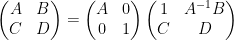

and on taking determinants using (1) we obtain the Schur determinant identity
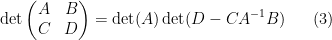
relating the determinant of a block-diagonal matrix with the determinant of the Schur complement  of the upper left block . This identity can be viewed as the correct way to generalise the
  determinant formula

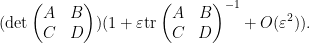
It is also possible to use determinant identities to deduce other matrix identities that do not involve the determinant, by the technique of matrix differentiation (or equivalently, matrix linearisation). The key observation is that near the identity, the determinant behaves like the trace, or more precisely one has

for any bounded square matrix and infinitesimal  . (If one is uncomfortable with infinitesimals, one can interpret this sort of identity as an asymptotic as
  .) Combining this with (1) we see that for square matrices of the same dimension with invertible and
  invertible, one has


for infinitesimal . To put it another way, if  is a square matrix that depends in a differentiable fashion on a real parameter
  , then we have the Jacobi formula
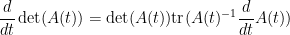
whenever is invertible. (Note that if one combines this identity with cofactor expansion, one recovers Cramer’s rule.)
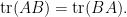
Let us see some examples of this differentiation method. If we take the Weinstein-Aronszajn identity (2) and multiply one of the rectangular matrices by an infinitesimal , we obtain

applying (4) and extracting the linear term in (or equivalently, differentiating at and then setting  ) we conclude the cyclic property of trace:
To manipulate derivatives and inverses, we begin with the Neumann series approximation

for bounded square and infinitesimal , which then leads to the more general approximation


for square matrices of the same dimension with  bounded. To put it another way, we have

whenever depends in a differentiable manner on and is invertible.
We can then differentiate (or linearise) the Schur identity (3) in a number of ways. For instance, if we replace the lower block by  for some test matrix
  , then by (4), the left-hand side of (3) becomes (assuming the invertibility of the block matrix)

while the right-hand side becomes

extracting the linear term in , we conclude that
As was an arbitrary matrix, we conclude from duality that the lower right block of  is given by the inverse
  of the Schur complement:

One can also compute the other components of this inverse in terms of the Schur complement  by a similar method (although the formulae become more complicated). As a variant of this method, we can perturb the block matrix in (3) by an infinitesimal multiple of the identity matrix giving

By (4), the left-hand side is
From (5), we have

and so from (4) the right-hand side of (6) is


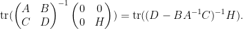
extracting the linear component in , we conclude the identity

which relates the trace of the inverse of a block matrix, with the trace of the inverse of one of its blocks. This particular identity turns out to be useful in random matrix theory; I hope to elaborate on this in a later post.
As a final example of this method, we can analyse low rank perturbations  of a large () matrix , where is an matrix and is an matrix for some
  . (This type of situation is also common in random matrix theory, for instance it arose in this previous paper of mine on outliers to the circular law.) If is invertible, then from (1) and (2) one has the matrix determinant lemma

if one then perturbs by an infinitesimal matrix  , we have

Extracting the linear component in as before, one soon arrives at

assuming that and are both invertible; as is arbitrary, we conclude (after using the cyclic property of trace) the Sherman-Morrison formula

for the inverse of a low rank perturbation of a matrix . While this identity can be easily verified by direct algebraic computation, it is somewhat difficult to discover this identity by such algebraic manipulation; thus we see that the “determinant first” approach to matrix identities can make it easier to find appropriate matrix identities (particularly those involving traces and/or inverses), even if the identities one is ultimately interested in do not involve determinants. (As differentiation typically makes an identity lengthier, but also more “linear” or “additive”, the determinant identity tends to be shorter (albeit more nonlinear and more multiplicative) than the differentiated identity, and can thus be slightly easier to derive.)
Exercise 1 Use the “determinant first” approach to derive the Woodbury matrix identity (also known as the binomial inverse theorem)

where is an matrix, is an matrix, is an matrix, and is an matrix, assuming that , and  are all invertible.
Exercise 2 Let be invertible matrices. Establish the identity

and differentiate this in to deduce the identity

(assuming that all inverses exist) and thence

Rotating by  then gives

which is useful for inverting a matrix  that has been split into a self-adjoint component and a skew-adjoint component
  .
.


45 comments
Comments feed for this article
13 January, 2013 at 12:51 pm
Mark Meckes
Thanks! I’m about to start teaching a matrix analysis course in which I was going to cover most of this material, though I hadn’t thought of quite this viewpoint on the second half. I think you’ve just saved me the work of preparing one lecture.
31 January, 2013 at 1:01 pm
Mark Meckes
I’m also delighted to discover that telling my browser to print this page results in a printout of the content of the post without all the links on the left.
13 January, 2013 at 1:00 pm
José Carlos Santos
When you wrote “{n+m \times n+m} square matrices”, what you meant was “{(n+m) \times (n+m)} square matrices”.
[Parentheses added – T.]
13 January, 2013 at 1:29 pm
Matrix identities as derivatives of determinant identities « Guzman's Mathematics Weblog
[…] via Matrix identities as derivatives of determinant identities. […]
13 January, 2013 at 2:30 pm
Anonymous
Should the matrix [1,C;0,1] above equation (3) be [1,0;C,1]?
[Corrected, thanks – T.]
13 January, 2013 at 4:43 pm
Joseph Nebus
I think I’m most startled to realize that I don’t remember having encountered Sylvester’s determinant identity before. It seems like a wonderful little bit to show off. (But I suppose everyone’s life is filled with wonderful little bits they run across only surprisingly late.)
13 January, 2013 at 10:29 pm
����Ԫ
Hello, I’m a big fan of Terry Tao’s “What’s new” blog, however mainland China has blocked the WordPress. Therefore, I would appreciate it very much if you could send me full copy of each new post better in PDF rather than just e-mail since the character won’t show up.
Send from Ted
6 February, 2013 at 6:31 am
I am not an anoymous
I use freegate + Autoproxy(a plugin of firefox) to circumvent the GFW,you can download freegate here:http://forums.internetfreedom.org/index.php?topic=18444.0
Also,there are several other ways to circumvent the great firewall of China,there are some discussion here:
14 January, 2013 at 10:11 am
Anonymous
Hi,
Is there a minus missing on the right-hand side of the equation below (5)? (the equation of the derivative of A(t) inverse)
[Corrected, thanks – T.]
14 January, 2013 at 3:24 pm
Peter
One identity that has been useful for me recently involves two matrices . The identity is
Out of curiosity, do you know if this can be derived using the methods you described? The identity isn’t hard to prove using the fact that a matrix satisfies its own characteristic polynomial, but I don’t know a very satisfying proof.
14 January, 2013 at 4:04 pm
Terence Tao
Hmm, that is a puzzle. It can be deduced by differentiating the matrix identity
which is valid for arbitrary matrices
  , in the
  direction (at
  ), but then I don’t know of a good reason (other than brute force calculation) as to why (*) holds, other than an observation that five quantities
  parameterise the
  -dimensional space of pairs
  of
of  matrices up to conjugation, so some identity of the form (*) ought to exist, and then degree considerations indicate that it should have the homogeneous structure indicated in (*).
1 February, 2014 at 10:37 am
Anonymous
The identity det(X + Y) = det(X) + det(Y) – tr(XY) + tr(X)tr(Y) is a special case of the identity described in Reutenauer and Schuetzenberger’s paper giving the determinant of the sum of k square matrices of order n as a sum of k^n terms. For example, if X and Y are 3×3 matrices then det(X + Y) = det(X) + det(Y) – tr(XY)tr(X) – tr(XY)tr(Y) + c(X)tr(Y) + tr(X)c(Y) + tr(XXY) + tr(XYY) , where c(X) = (tr(X)^2 – tr(X^2)) / 2.
18 January, 2013 at 2:04 am
Gil Kalai
One thing that comes to mind in this context are polynomial identities for the ring of matrices like the Amitsur-Levitzki identity (See, e.g. http://gilkalai.wordpress.com/2009/05/12/the-amitsur-levitski-theorem-for-a-non-mathematician/ ) For those there is a result by Processi and by Razmislov which asserts that all PI identities are derived from the Cayley-Hamilton theorem, which is a sort of determinant-identity.
18 January, 2013 at 2:49 pm
A researcher
Hello Gil, would you be able to give us a suitable source for the Processi or Razmislov works? Further, could you explain what do you mean by “all PI identities are derived from the C-H theorem”? I thought that to find the generating set of all PI identities of the ring of matrices is an open problem. Only for 2×2 matrices it was solved by Drenski in 1981. But maybe we’re talking about different definitions?
19 January, 2013 at 9:44 am
Gil Kalai
Perhaps for the results I mentioned “are derived” is quite a description of generating sets.
There is an article “Polynomial identities and the Cayley-Hamilton theorem” by Edward Formanek in The Mathematical Intelligencer 11(89) 37-39 which describes the related works of Processi and Razmislov. Rowen’s BAMS book review of a book by Formanek and Drensky http://www.ams.org/bull/2006-43-02/S0273-0979-06-01082-2/S0273-0979-06-01082-2.pdf contains a lot of interesting information.
19 January, 2013 at 8:17 am
Nick Higham
There are lots of nice result along these lines. One of my favorites is for any
 and
and 
 such that both matrix functions (where
  maps square matrices to square matrices) are defined. In particular,
  . The proofs are easy using the theory of matrix functions (see Section 1.8 of http://www.maths.manchester.ac.uk/~higham/fm/index.php).
21 January, 2013 at 3:08 am
Anonymous
As usual, a wonderful to learn from exposition. I was thinking if Prof. Tao could have also related determinant (det) to the rank function. I mean, the current literature suggests det as a good surrogate for the rank, than, for example, the trace function. Probably, this could have motivated some tighter approximations for the rank operator which can be immensely useful, for instance, in numerical optimization. Of course, other application for this very aspect arises in compressive sensing, and, Prof. Tao is again a seminal contributor in this area of signal processing!
30 January, 2013 at 4:26 pm
Amit Bhaya
There’s also the lovely and well known formula \det \exp A = \exp trace(A) with its connection to Liouville’s theorem on conservation of phase space volume by Hamiltonian flows (since Hamiltonian matrices have zero trace).
31 January, 2013 at 3:23 pm
teobanica
Hello, I’m teaching some linear algebra this semester, and, as always, quite hard to get through the first definitions, as to be able to start speaking about the magics of .. There’s actually this problem with the very definition of
  : is that a volume (intuitive and nice and everything), or some more abstract thing? I learned in Romania, using abstract stuff, now I’m teaching in France, and I have to use abstract stuff as well (otherwise I’d be probably put on the death row by my colleagues :) On the other hand a Russian colleague of mine told me that, at least some 20 years ago,
  was by definition a volume, in Moscow! (that’s probably why Russians are so good at it) I was wondering how the situation in the US is: any choice allowed? For math students of course.
5 February, 2013 at 2:39 pm
anonymous
Dear Professor Tao,
I did the calculation of the products of the two matrices X and Y, and it does not seem to give the Sylvester determinant equaltiy. Could this point be further elaborated on?
5 February, 2013 at 6:47 pm
Terence Tao
Oops, I didn’t set up the matrices correctly. It should be OK now…
23 July, 2013 at 11:33 am
Mike
If I’m not missing something, I think you really wanted the second product to simply be the first one in reverse order, instead of using the matrix with a 0 and a -B.
[Corrected, thanks – T.]
14 February, 2013 at 6:47 am
Artificial Intelligence Blog · “Matrix identities as derivatives of determinant identities”
[…] Check out Terence Tao‘s wonderful post ”Matrix identities as derivatives of determinant identities“. […]
17 February, 2013 at 10:54 pm
Craig Tracy
For an account of the use of the Sylvester det identity, det(I+AB)=det(I+BA), in random matrix theory, see C. Tracy & H. Widom, “Correlation functions, cluster functions and spacing distributions for random matrices”, J. of Statistical Physics 92 (1998) 809-835.
Click to access CV59.pdf
19 February, 2013 at 8:57 pm
Supercommutative gaussian integration, and the gaussian unitary ensemble « What’s new
[…] later in this post. By the trick of matrix differentiation of the determinant (as reviewed in this recent blog post), one can also use this method to compute matrix-valued statistics such […]
3 April, 2013 at 12:02 pm
Study Hacks » Blog Archive » You Can Be Busy or Remarkable — But Not Both
[…] new year, he’s written nine long posts, full of mathematical equations and fun titles, like “Matrix identities as derivatives of determinant identities.” His most recent post is 3700 words long! And that’s a normal […]
15 January, 2014 at 11:32 am
Kyle Kloster
I’m having trouble with the derivation of the block inverse form, above (6): in (3) now appears as
  , and I can’t figure out why. Then, equating the linear terms in
  is said to yield
the term
I don’t understand what happened to the other coefficients of these linear terms, for the right-hand side, and
 ![\hbox{det}( [ A, B; C, D] )](https://s0.wp.com/latex.php?latex=%5Chbox%7Bdet%7D%28+%5B+A%2C+B%3B+C%2C+D%5D+%29&bg=ffffff&fg=545454&s=0&c=20201002) for the left-hand side.
for the left-hand side.
What am I missing?
15 January, 2014 at 1:42 pm
Terence Tao
Oops, there were some typos in the text (in particular, all occurrences of , which doesn’t even make sense as a matrix product, should be
  instead); hopefully they are corrected now.
15 January, 2014 at 1:48 pm
Kyle Kloster
Thanks for the response!
There is still one occurrence of $BA^{-1}C$, in the paragraph immediately prior to equation (6).
[Corrected, thanks – T.]
15 January, 2014 at 2:21 pm
Anonymous
Typo: Exercise 2: “thence” –> “hence”.
[Corrected, thanks – T.]
20 April, 2014 at 9:50 am
My Math Diary
[…] Derivative of determinant: Terry Tao, Stack […]
24 September, 2014 at 2:29 pm
Derived multiplicative functions | What's new
[…] identities, such as (1). This phenomenon is analogous to the one in linear algebra discussed in this previous blog post, in which many of the trace identities used there are derivatives of determinant identities. For […]
3 April, 2017 at 6:31 pm
Pascal
Hi, may i know is there any analytic formula for the derivative of adjugate matrix w.r.t itself or its elements? i.e.
or
22 May, 2017 at 5:55 pm
Quantitative continuity estimates | What's new
[…] is a scalar such that is non-zero. (See also this previous blog post for more discussion of these sorts of […]
4 June, 2017 at 12:06 am
起源笔记 / 基于云数据的网络松鼠症分布模型设计一文
[…] a scalar such that is non-zero. (See also this previous blog post for more discussion of these sorts of […]
23 July, 2017 at 11:25 pm
user777
Is it possible to have any such derivations for permanent-trace or permanent-determinant?
28 August, 2017 at 1:17 pm
Dodgson condensation from Schur complementation | What's new
[…] can in turn be used to establish many further identities; in particular, as shown in A HREF=”https://terrytao.wordpress.com/2013/01/13/matrix-identities-as-derivatives-of-determinant-identities… previous post, it implies the Schur determinant […]
16 September, 2017 at 2:07 pm
Inverting the Schur complement, and large-dimensional Gelfand-Tsetlin patterns | What's new
[…] the other hand, by the Woodbury matrix identity (discussed in this previous blog post), we […]
17 October, 2017 at 10:51 am
Anonymous
Is there any book which discusses this stuff and particularly identity 4 and its corresponding identity
1 August, 2018 at 3:30 am
Chris
how can I find the derivative of det(I-2itA∑) ? Please help!
21 August, 2018 at 8:41 am
DREAM PETER SARNAK 21 AUGUST 2018 | zulfahmed
[…] what is necessary to understand is the relation between determinant and trace and Terry has a very nice article clarifying these issues so we can understand the relations clearly: “The key observation is […]
13 April, 2019 at 6:57 pm
Leonardo Torres
What is a reference for (4)?
13 April, 2019 at 9:02 pm
Anonymous
characteristic polynomial
12 November, 2021 at 12:05 am
Gilad Lerman
Typo: In Exercise 2 the minus sign between the two inverses in the last two equations should be a plus sign (just found these notes when searching for material relevant for some teaching notes I write and I like it)
[Minus sign in the third equation corrected; the minus sign in the fourth equation however appears to be correct – T.]
12 November, 2021 at 8:44 am
Gilad Lerman
yes, of course (I focused on the third line)