
Define a partition of 

![{I \in (0,1]}](https://s0.wp.com/latex.php?latex=%7BI+%5Cin+%280%2C1%5D%7D&bg=ffffff&fg=000000&s=0&c=20201002)


- (Prime factorisation) Given a natural number
, one can decompose it into prime factors
(counting multiplicity), and then the multiset
is a partition of
- (Cycle decomposition) Given a permutation
on
, one can decompose
into cycles
, and then the multiset
is a partition of
- (Normalisation) Given a multiset
of positive real numbers whose sum
is finite and non-zero, the multiset
is a partition of
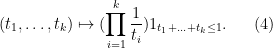
In the spirit of the universality phenomenon, one can ask what is the natural distribution for what a “typical” partition should look like; thus one seeks a natural probability distribution on the space of all partitions, analogous to (say) the gaussian distributions on the real line, or GUE distributions on point processes on the line, and so forth. It turns out that there is one natural such distribution which is related to all three examples above, known as the Poisson-Dirichlet distribution. To describe this distribution, we first have to deal with the problem that it is not immediately obvious how to cleanly parameterise the space of partitions, given that the cardinality of the partition can be finite or infinite, that multiplicity is allowed, and that we would like to identify two partitions that are permutations of each other
One way to proceed is to random partition 
![\displaystyle N_{[a,b]} := |\Sigma \cap [a,b]| = \sum_{x \in\Sigma} 1_{[a,b]}(x)](https://s0.wp.com/latex.php?latex=%5Cdisplaystyle+N_%7B%5Ba%2Cb%5D%7D+%3A%3D+%7C%5CSigma+%5Ccap+%5Ba%2Cb%5D%7C+%3D+%5Csum_%7Bx+%5Cin%5CSigma%7D+1_%7B%5Ba%2Cb%5D%7D%28x%29&bg=ffffff&fg=000000&s=0&c=20201002)
(where the cardinality here counts multiplicity). This can certainly be done, although in the case of the Poisson-Dirichlet process, the formulae for the joint distribution of such counting functions is moderately complicated. Another way to proceed is to order the elements of
with the convention that one pads the sequence 
![\displaystyle \{ (t_1,t_2,\ldots) \in [0,1]^{\bf N}: t_1 \geq t_2 \geq \ldots; \sum_{n=1}^\infty t_n = 1 \}.](https://s0.wp.com/latex.php?latex=%5Cdisplaystyle+%5C%7B+%28t_1%2Ct_2%2C%5Cldots%29+%5Cin+%5B0%2C1%5D%5E%7B%5Cbf+N%7D%3A+t_1+%5Cgeq+t_2+%5Cgeq+%5Cldots%3B+%5Csum_%7Bn%3D1%7D%5E%5Cinfty+t_n+%3D+1+%5C%7D.&bg=ffffff&fg=000000&s=0&c=20201002)
However, it turns out that the process of ordering the elements is not “smooth” (basically because functions such as 
It turns out that there is a better (or at least “smoother”) way to enumerate the elements 
- Given a partition
be an element of
having a probability
of being chosen as
occurs with multiplicity
, the net probability that
). Note that this is well-defined since the elements of
- Now suppose
is empty, we set
all equal to zero and stop. Otherwise, let
be an element of
chosen at random, with each element
having a probability
in
with probability
.)
- Now suppose
are both chosen. If
is empty, we set
all equal to zero and stop. Otherwise, let
be an element of
, with ech element
having a probability
- We continue this process indefinitely to create elements
.
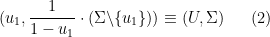
We denote the random sequence ![{Enum(\Sigma) := (u_1,u_2,\ldots) \in [0,1]^{\bf N}}](https://s0.wp.com/latex.php?latex=%7BEnum%28%5CSigma%29+%3A%3D+%28u_1%2Cu_2%2C%5Cldots%29+%5Cin+%5B0%2C1%5D%5E%7B%5Cbf+N%7D%7D&bg=ffffff&fg=000000&s=0&c=20201002)
![{[0,1]^{\bf N}}](https://s0.wp.com/latex.php?latex=%7B%5B0%2C1%5D%5E%7B%5Cbf+N%7D%7D&bg=ffffff&fg=000000&s=0&c=20201002)

with 

Note that one can recover 

with the convention that one discards any zero elements on the right-hand side. Thus 
Note that this random enumeration procedure can also be adapted to the three models described earlier:
- Given a natural number
by letting each prime factor
of
with probability
, then once
be equal to
with probability
, and so forth.
- Given a permutation
, one can randomly enumerate its cycles
by letting each cycle
in
with probability
, and once
with probability
, and so forth. Alternatively, one traverse the elements of
- Given a multiset
is finite, we can randomly enumerate
the elements of this sequence by letting each
have a
probability of being set equal to
, and then once
have a
probability of being set equal to
, and so forth.
We then have the following result:
Proposition 1 (Existence of the Poisson-Dirichlet process) There exists a random partition
has the uniform distribution on
are independently and identically distributed copies of the uniform distribution on
.
A random partition

where 
An equivalent definition of a Poisson-Dirichlet process is a random partition
where 


It turns out that each of the three ways to generate partitions listed above can lead to the Poisson-Dirichlet process, either directly or in a suitable limit. We begin with the third way, namely by normalising a Poisson process to have sum
Proposition 2 (Poisson-Dirichlet processes via Poisson processes) Let
, and let
be a Poisson process on
with intensity function
. Then the sum
is almost surely finite, and the normalisation
is a Poisson-Dirichlet process.
Again, we prove this proposition below the fold. Now we turn to the second way (a topic, incidentally, that was briefly touched upon in this previous blog post):
Proposition 3 (Large cycles of a typical permutation) For each natural number
. Then the random partition
converges in the limit
to a Poisson-Dirichlet process
in the following sense: given any fixed sequence of intervals
(independent of
converges in distribution to
.
Finally, we turn to the first way:
Proposition 4 (Large prime factors of a typical number) Let
, and let
be a random natural number chosen according to one of the following three rules:
- (Uniform distribution)
.
- (Shifted uniform distribution)
.
- (Zeta distribution) Each natural number
of being equal to
and
.
Then
converges as
to a Poisson-Dirichlet process
The process
The previous two propositions suggests an interesting analogy between large random integers and large random permutations; see this ICM article of Vershik and this non-technical article of Granville (which, incidentally, was once adapted into a play) for further discussion.
As a sample application, consider the problem of estimating the number 


![{[1/u,1]}](https://s0.wp.com/latex.php?latex=%7B%5B1%2Fu%2C1%5D%7D&bg=ffffff&fg=000000&s=0&c=20201002)


I thank Andrew Granville and Anatoly Vershik for showing me the nice link between prime factors and the Poisson-Dirichlet process. The material here is standard, and (like many of the other notes on this blog) was primarily written for my own benefit, but it may be of interest to some readers. In preparing this article I found this exposition by Kingman to be helpful.
Note: this article will emphasise the computations rather than rigour, and in particular will rely on informal use of infinitesimals to avoid dealing with stochastic calculus or other technicalities. We adopt the convention that we will neglect higher order terms in infinitesimal calculations, e.g. if 

— 1. Constructing the Poisson-Dirichlet process —
We now prove Proposition 2, which of course also implies Proposition 1.
Let 


We first understand the law of the sum 
Lemma 5 Let
is an exponential variable with probability distribution
. In particular,
is almost surely finite.
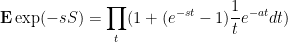
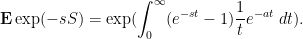
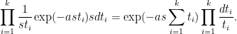
Proof: Taking Laplace transforms, it suffices to show that

for all 


(ignoring higher order terms) and thus

and thus on sending
The quantity 


and (3) follows.
The same analysis can be performed for Poisson processes with more general intensity functions, leading to Campbell’s theorem. However, the exponential nature of

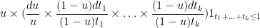
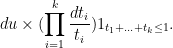
Proposition 6 Let
Proof: Let ![{[t_1,t_1+dt_1],\ldots,[t_k,t_k+dt_k]}](https://s0.wp.com/latex.php?latex=%7B%5Bt_1%2Ct_1%2Bdt_1%5D%2C%5Cldots%2C%5Bt_k%2Ct_k%2Bdt_k%5D%7D&bg=ffffff&fg=000000&s=0&c=20201002)
![{[s,s+ds]}](https://s0.wp.com/latex.php?latex=%7B%5Bs%2Cs%2Bds%5D%7D&bg=ffffff&fg=000000&s=0&c=20201002)


![{[t_i,t_i+dt_i]}](https://s0.wp.com/latex.php?latex=%7B%5Bt_i%2Ct_i%2Bdt_i%5D%7D&bg=ffffff&fg=000000&s=0&c=20201002)


![{[st_i,st_i+sdt_i]}](https://s0.wp.com/latex.php?latex=%7B%5Bst_i%2Cst_i%2Bsdt_i%5D%7D&bg=ffffff&fg=000000&s=0&c=20201002)

![{[s-x_1-\ldots-x_k,s-x_1-\ldots-x_k+ds]}](https://s0.wp.com/latex.php?latex=%7B%5Bs-x_1-%5Cldots-x_k%2Cs-x_1-%5Cldots-x_k%2Bds%5D%7D&bg=ffffff&fg=000000&s=0&c=20201002)
Once we condition on this event, 


Since 
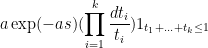
giving the claim.
Note that the above calculation in fact computes the 

We can now show the Poisson-Dirichlet property (2):
Proposition 7 Let
, and let
be a random element, with each
has the same distribution as
Proof: We first establish that 
![{[u,u+du]}](https://s0.wp.com/latex.php?latex=%7B%5Bu%2Cu%2Bdu%5D%7D&bg=ffffff&fg=000000&s=0&c=20201002)


Now consider the probability of the event 


![{u_1 \in [u,u+du]}](https://s0.wp.com/latex.php?latex=%7Bu_1+%5Cin+%5Bu%2Cu%2Bdu%5D%7D&bg=ffffff&fg=000000&s=0&c=20201002)
![{[(1-u)t_i, (1-u)t_i+(1-u)dt_i]}](https://s0.wp.com/latex.php?latex=%7B%5B%281-u%29t_i%2C+%281-u%29t_i%2B%281-u%29dt_i%5D%7D&bg=ffffff&fg=000000&s=0&c=20201002)


which simplifies to
If we condition out by
Remark 8 As a crude zeroth approximation to the process
, one can consider the Poisson process
on
. By (4), this process has the same
is replaced by
). Related to this,
should equal
has an independent probability of
of dividing
Remark 9 If one starts with a Poisson process
of intensity
for some parameter
and normaliises it as above, one arrives at a more general Poisson-Dirichlet process whose enumeration variables
— 2. Cycle decomposition of random permutations —
The proof of Proposition 3 is essentially immediate from the following claim:
Proposition 10 Let
and
be as in Proposition 3. Let
, with each
occuring with probability
of
, and after conditioning on a given value
of
has the distribution of
.
Heuristically at least, in the limit 
Proof: We first compute the probability that 


The same analysis shows that once one fixes the cycle of length
— 3. Asymptotics of prime divisors —
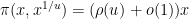
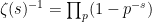
We now prove Proposition 4. We first give a simple argument of Lloyd (as described by Kingman), which handles the much smoother (and hence much easier) third case of the theorem. In this case one can take advantage of Euler product factorisation. Indeed, if we define 


Now we prove the theorem in the first and second cases. Here, the Euler product factorisation is not available (unless one allows
Proposition 11 Let
be a random prime factor of
of being chosen as
converges in the vague topology to the uniform distribution as
of
has the same distribution as
(up to negligible errors).
Again, upon taking logarithms and sending
Proof: (Informal) For sake of concreteness let us work with the second case of Proposition 4, as the first case is similar (and also follows from the second case by a dyadic decomposition). We compute the probability that 
![\displaystyle \frac{1}{x} \times \frac{\log p}{\log N_x} 1_{[x,2x]}(pm) \approx\frac{1}{p} \frac{\log p}{\log x} \frac{1}{x/p} 1_{[x/p,2x/p]}(m).](https://s0.wp.com/latex.php?latex=%5Cdisplaystyle+%5Cfrac%7B1%7D%7Bx%7D+%5Ctimes+%5Cfrac%7B%5Clog+p%7D%7B%5Clog+N_x%7D+1_%7B%5Bx%2C2x%5D%7D%28pm%29+%5Capprox%5Cfrac%7B1%7D%7Bp%7D+%5Cfrac%7B%5Clog+p%7D%7B%5Clog+x%7D+%5Cfrac%7B1%7D%7Bx%2Fp%7D+1_%7B%5Bx%2Fp%2C2x%2Fp%5D%7D%28m%29.&bg=ffffff&fg=000000&s=0&c=20201002)
(This is slightly inaccurate in the case that
Summing in 

![{[a,b]}](https://s0.wp.com/latex.php?latex=%7B%5Ba%2Cb%5D%7D&bg=ffffff&fg=000000&s=0&c=20201002)
which by Mertens’ theorems is asymptotic to 
Remark 12 The same argument also works when
Remark 13 A variant of Proposition 4 of relevance to the polymath8 project; if instead of selecting
has a probability
of being chosen as
, where
is the number of prime factors of
is now asymptotic to a generalised Poisson-Dirichlet process in which the coordinates
rather than the uniform distribution. (This distribution is in fact of the form in Remark 9, with
replaced by
.) In particular, when
), which helps explain the Motohashi-Pintz-Zhang phenomenon that when sieving for
— 4. Dickman’s function —
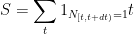
Let 


Let 


![{S \in [(u-du)T_*, uT_*]}](https://s0.wp.com/latex.php?latex=%7BS+%5Cin+%5B%28u-du%29T_%2A%2C+uT_%2A%5D%7D&bg=ffffff&fg=000000&s=0&c=20201002)

For any real number 

![{T_* \in [t_*, t_*+dt]}](https://s0.wp.com/latex.php?latex=%7BT_%2A+%5Cin+%5Bt_%2A%2C+t_%2A%2Bdt%5D%7D&bg=ffffff&fg=000000&s=0&c=20201002)

![{[t_*, t_*+dt_*]}](https://s0.wp.com/latex.php?latex=%7B%5Bt_%2A%2C+t_%2A%2Bdt_%2A%5D%7D&bg=ffffff&fg=000000&s=0&c=20201002)

![{S - t'_* \in [(u-du-1)t_*, (u-1)t_*]}](https://s0.wp.com/latex.php?latex=%7BS+-+t%27_%2A+%5Cin+%5B%28u-du-1%29t_%2A%2C+%28u-1%29t_%2A%5D%7D&bg=ffffff&fg=000000&s=0&c=20201002)


which simplifies to 


Remark 14 Using (4) and the inclusion-exclusion formula, one also has the integral expression
for
term is
and so only finitely many terms in this expression need to be evaluated. This gives another way to verify the delay-differential equation
.


27 comments
Comments feed for this article
24 September, 2013 at 7:05 am
arch1
In step 2 of the enumeration procedure, why isn’t the probability of equaling
  instead
  , since there are
  instances of
  remaining in the multiset at that point, each of which has probability
  of being chosen?
[Oops, that was a careless mistake; fixed now, thanks. -T.]
24 September, 2013 at 5:53 pm
D
The steps 2–4 do not agree with the reconstruction in formula (1). When you pick u_1, do you divide remaining points by 1-u_1? In other words, u_2 does not come from the original list \Sigma, but from a rescaled list?
[Oops, you’re right; the way it was written was completely confusing. I hope I’ve fixed it now – T.]
26 September, 2013 at 5:19 am
arch1
In the recursive formula for Enum, should the multiplier therefore be ?
?
[Corrected, thanks – T.]
12 February, 2020 at 9:52 pm
Peleg Michaeli پليج (@pelegmichaeli)
I think this is still written wrongly, or at least unclear. Suppose , and suppose
  . Then
  is chosen from
  . Now suppose
  . You probably don’t want to have
  in the denominator in step 3.
[Corrected, thanks – T.]
25 September, 2013 at 9:57 am
David
This Poisson-Dirichlet process is PD(1) in a more general family PD(t), see page 99 of Poisson processes by Kingman. The same construction, only the uniform distribution is replaced by Beta(1,t) distribution. The process PD(t) itself is PD(0,t) in more general family PD(a,t) in the paper of Pitman and Yor.
25 September, 2013 at 9:59 am
D
In Proposition 6, equality sign is missing in {\Sigma_N(\Gamma_a) = \frac{1}{S} \cdot \Gamma_a}.
[Corrected, thanks – T.]
25 September, 2013 at 11:04 am
❧ ✲ ❂ ❂ ✲✳ ✴ ✶ ❂✯❀
In Proposition 4, \Sigma_{PD} is \Sigma_{PF}.
[Corrected, thanks – T.]
25 September, 2013 at 6:44 pm
D
In the case of Zeta distribution, the comment after the proof of Theorem 1 in Kingman’s paper implies that (asymptotically in x) multiplicities of any finite number of largest prime divisors are equal to one. I am assuming this also holds in the case 1 of Uniform distribution, so is it some basic result in number theory that the density of numbers with this property is equal to one? How can the number of largest prime divisors grow with x so that one still has this property?
25 September, 2013 at 8:01 pm
Terence Tao
Yes, it is rare for a large number to be divisible by a large prime with multiplicity more than one. This is basically because the sum is convergent, so that the sum
  goes to zero as
  goes to infinity. Thus, the proportion of numbers which are divisible by the square of a prime greater than
  goes to zero as
  goes to infinity. Among other things, this shows that the set of numbers whose largest
  prime factors occur with multiplicity one, has density one for any fixed
  .
.
5 October, 2013 at 3:36 pm
vcp
In the first sentence following the box containing Proposition 4, “by first done” can be deleted.
[Corrected, thanks – T.]
15 October, 2013 at 8:37 pm
thichchaytron
It very difficulty with me :(
17 October, 2013 at 12:28 pm
X
I think that there are some typos in section 1: Resp. 2 and 3 equations below (3), the left-hand side should be E exp(-sS), not E exp(-tS)
Also, “Theorem 2/3” should be “as in Proposition 2/3”
[Corrected, thanks – T.]
5 November, 2013 at 1:17 pm
Anita
Is it trivial that if they are non-zero and sums to 1, the multiset must be countable?
6 November, 2013 at 10:47 pm
Anita
Of course it is, ignore this.
13 November, 2013 at 3:30 am
Grigory F
Typo in the third line after equation (1):![[0,1]^n](https://s0.wp.com/latex.php?latex=%5B0%2C1%5D%5En&bg=ffffff&fg=545454&s=0&c=20201002) should read
should read ![[0,1]^{\bf N}](https://s0.wp.com/latex.php?latex=%5B0%2C1%5D%5E%7B%5Cbf+N%7D&bg=ffffff&fg=545454&s=0&c=20201002) instead.
instead.
[Corrected, thanks – T.]
21 November, 2013 at 5:33 pm
Sary D
Some signs should probably be swapped in section 4 : $u\rho'(u)=-\rho(u-1)$ and probability $-du\rho'(u)$, since rho is decreasing.
I love reading your blog !
[Corrected, thanks – T.]
14 March, 2014 at 11:16 am
The Chinese Restaurant Process | Eventually Almost Everywhere
[…] The Poisson-Dirichlet process, and large prime factors of a random number (terrytao.wordpress.com) […]
14 March, 2014 at 11:17 am
Urns and the Dirichlet Distribution | Eventually Almost Everywhere
[…] The Poisson-Dirichlet process, and large prime factors of a random number (terrytao.wordpress.com) […]
15 July, 2015 at 2:44 pm
Cycles of a random permutation, and irreducible factors of a random polynomial | What's new
[…] If is a randomly selected large integer of size , and is a randomly selected prime factor of (with each index being chosen with probability ), then is approximately uniformly distributed between and . (See Proposition 9 of this previous blog post.) […]
18 March, 2016 at 12:07 am
saroj
can any body give me the proof of ”(estimation of s^(2/B))<infinite''????
16 August, 2018 at 10:40 am
Karl Keppler
Dickman function arises in a problem proposed here:
https://math.stackexchange.com/questions/2130264/sum-of-random-decreasing-numbers-between-0-and-1-does-it-converge
31 October, 2018 at 8:53 am
Martin
Hi Terry!
Your blog post asked what’s new in prime numbers. I have something I think is new I would like to show you and the readers of your blog. I hope you don’t mind and are gracious enough to post this.
Kind regards,
Martin
Claim: “All prime numbers can be transformed into an integer sequence equivalent to one-half the sum of the first 2n + 1 primes.”
Proof:
1) Sum each consecutive pair of prime numbers (i.e. 2,3 then 3,5, etc.)
2) Subtract the difference between the two numbers.
3) Divide the result by 4.
4) Keep a continual sum from step 3.
5) At odd intervals the continual sum is equivalent to 1/2 half the sum of the first 2n + 1 primes.
1, 5, 14, 29, 50, 80, 119, 164, 220, 284, 356, 437, 530, 632, 740, 860, 994, 1138, 1292, 1457, 1633, 1819, 2014, 2219, 2444, 2675, 2915, 3169, 3435
30 December, 2019 at 8:53 am
Separating big sticks from little sticks, and applications – Random Permutations
[…] Tao on the stick-breaking process, or the Poisson–Dirichlet process (which is essentially the same); […]
30 March, 2020 at 9:37 am
Noam
I think there is a mistake in the calculation of the integral that appears in the proof that S is an exponential variable – I believe it should be log(a/(s+a)) and not – log(s+a).
[Corrected, thanks – T.]
3 October, 2020 at 7:38 am
Will
Some kind of malformed formatting tag in the proof of Proposition 7 has gone mad with power and underlined half this post.
[Corrected, thanks – T.]
6 March, 2024 at 9:35 am
Anonymous
This is a wonderful blog post and I really enjoyed the read! However, I am struggling to understand few things regarding the proof of Lemma 5.
– Given the definition of exponential r.v. in the lemma, shouldn’t we show – in (3) – that its Laplace transform is a/(s+a)?
– Why is \Gamma_a=a\Gamma_1? Already by checking the expectation of the two processes, the integrand looks different.
– I don’t understand how can we rewrite the Laplace transform of S as the product in the third equation of the proof for Lemma 5. Isn’t S given by a Poisson binomial distribution?
Thanks in advance for the clarifications. FZ
17 March, 2024 at 6:14 pm
Terence Tao
1. This was a typo, now corrected. should be
  .
.
2. This was also a typo:
3. The Laplace transform (aka moment generating function) of a sum of independent random variables is the product of the Laplace transform of the individual variables.