This is the third thread for the Polymath8b project to obtain new bounds for the quantity
either for small values of  (in particular
  ) or asymptotically as
  . The previous thread may be found here. The currently best known bounds on
  are:
are:
- (Maynard) Assuming the Elliott-Halberstam conjecture,
 .
.
- (Polymath8b, tentative)
 . Assuming Elliott-Halberstam,
  .
.
- (Polymath8b, tentative)
 . Assuming Elliott-Halberstam,
  .
.
- (Polymath8b)
 for sufficiently large . Assuming Elliott-Halberstam,
  for sufficiently large .
Much of the current focus of the Polymath8b project is on the quantity
where  ranges over square-integrable functions on the simplex

with  being the quadratic forms
and

It was shown by Maynard that one has  whenever
  , where
  is the narrowest diameter of an admissible
  -tuple. As discussed in the previous post, we have slight improvements to this implication, but they are currently difficult to implement, due to the need to perform high-dimensional integration. The quantity
  does seem however to be close to the theoretical limit of what the Selberg sieve method can achieve for implications of this type (at the Bombieri-Vinogradov level of distribution, at least); it seems of interest to explore more general sieves, although we have not yet made much progress in this direction.
The best asymptotic bounds for we have are

which we prove below the fold. The upper bound holds for all  ; the lower bound is only valid for sufficiently large , and gives the upper bound
  on Elliott-Halberstam.
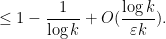
For small , the upper bound is quite competitive, for instance it provides the upper bound in the best values
and

we have for  and
and  . The situation is a little less clear for medium values of , for instance we have

and so it is not yet clear whether  (which would imply
  ). See this wiki page for some further upper and lower bounds on .
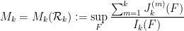
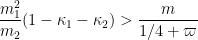
The best lower bounds are not obtained through the asymptotic analysis, but rather through quadratic programming (extending the original method of Maynard). This has given significant numerical improvements to our best bounds (in particular lowering the  bound from
  to
to  ), but we have not yet been able to combine this method with the other potential improvements (enlarging the simplex, using MPZ distributional estimates, and exploiting upper bounds on two-point correlations) due to the computational difficulty involved.
— 1. Upper bound —
We now prove the upper bound in (1). The key estimate is


Assuming this estimate, we may integrate in  to conclude that

which symmetrises to

giving the upper bound in (1).
It remains to prove (2). By Cauchy-Schwarz, it suffices to show that

But writing  , the left-hand side evaluates to
as required.
This also suggests that extremal  behave like
  for some function
  , and similarly for permutations. However, it is not possible to have exact equality in all variables simultaneously, which indicates that the upper bound (1) is not optimal, although in practice it does remarkably well for small .
— 2. Lower bound —
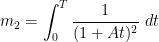
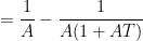
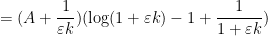
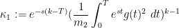
Using the notation of this previous post, we have the lower bound
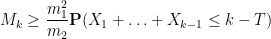
whenever  is supported on
 ![{[0,T]}](https://s0.wp.com/latex.php?latex=%7B%5B0%2CT%5D%7D&bg=ffffff&fg=000000&s=0&c=20201002) ,
,  , and
, and  are independent random variables on with density
  . We select the function
![\displaystyle g(t) := \frac{1}{1 + A t} 1_{[0,T]}(t)](https://s0.wp.com/latex.php?latex=%5Cdisplaystyle+g%28t%29+%3A%3D+%5Cfrac%7B1%7D%7B1+%2B+A+t%7D+1_%7B%5B0%2CT%5D%7D%28t%29&bg=ffffff&fg=000000&s=0&c=20201002)
with  , and
, and  for some
  to be chosen later. We have

and

and so

Observe that the random variables  have mean

The variance  may be bounded crudely by


Thus the random variable  has mean at most
  and variance
  , with each variable bounded in magnitude by
  . By Hoeffding’s inequality, this implies that is at least
  with probability at most
  for some absolute constant
  . If we set
  for a sufficiently large absolute constant
  , we thus have

and thus

giving the lower bound in (1).
Hoeffding’s bound is proven by the exponential moment method, which more generally gives the bound

for any  . However, this bound is inferior to the linear algebra method for small ; for instance, we can only obtain
 ![{DHL[k,2]}](https://s0.wp.com/latex.php?latex=%7BDHL%5Bk%2C2%5D%7D&bg=ffffff&fg=000000&s=0&c=20201002) for
for  by this method (compared to
  from quadratic programming), even if one uses the best available MPZ estimate.
Using ![{MPZ[\varpi,\delta]}](https://s0.wp.com/latex.php?latex=%7BMPZ%5B%5Cvarpi%2C%5Cdelta%5D%7D&bg=ffffff&fg=000000&s=0&c=20201002) , one can modify this lower bound, obtaining
, one can modify this lower bound, obtaining ![{DHL[k_0,m+1]}](https://s0.wp.com/latex.php?latex=%7BDHL%5Bk_0%2Cm%2B1%5D%7D&bg=ffffff&fg=000000&s=0&c=20201002) whenever we can find
whenever we can find  obeying
where
and
with


Details can be found at this comment.
— 3. Quadratic programming —
The expressions  ,
,  are quadratic forms in , so one can (in principle, at least) obtain lower bounds for by restricting to a finite-dimensional space of and performing quadratic programming on the resulting finite-dimensional quadratic forms.
One can take to be symmetric without loss of generality. One can then look at functions that are linear combinations of symmetric polynomials

for various signatures  ; actually it turns out numerically that one can get more efficient results by working with combinations of
  for
for  up to a fixed degree, and
  for at that degree afterwords, where
  is the first symmetric polynomial. (Note that the GPY type sieves come from the case when is purely a function of
  .)
.)
It may be that other choices of bases here are more efficient still (perhaps choosing bases that reflect the belief that should behave something like  for some smallish
  ), but one numerical obstacle is that we are only able to accurately compute the required coefficients for
  in the case of polynomials.


154 comments
Comments feed for this article
8 December, 2013 at 5:08 pm
Andrew Sutherland
A couple of minor typos in the bulleted list of bounds: I think should be
  and
and  should be
  .
.
8 December, 2013 at 5:19 pm
Terence Tao
Actually, the Elliott-Halberstam conjecture essentially allows us to double the value of for any bound previously obtained using only the Bombieri-Vinogradov theorem (such as the bound
  ).
).
8 December, 2013 at 5:11 pm
Terence Tao
This doesn’t directly help the numerical optimisation, but here is an alternate way to compute the integrals of polynomials on the simplex , giving a slightly different way to establish Lemma 7.1 from Maynard’s paper. The starting point is the identity
which is a simple application of Fubini’s theorem. If F is homogeneous of degree d, then
from the Gamma function identity , we thus see that
Now, from the gamma function identity again we have
and thus
Replacing k with , and then performing the
  integral, one also has the generalisation
which is equation (7.4) in Maynard’s paper.
This calculation suggests that Laplace transforms in the variables may possibly be useful.
8 December, 2013 at 5:51 pm
Terence Tao
I’ve been experimenting with the problem of optimising a sieve, to get some sense as to how sharp the Selberg sieve is. A model problem is the following: suppose one has a non-negative sequence for which one has the exact bounds
for all and some multiplicative function
  taking values in [0,1] and some quantity
  (in practice there are error terms also, but I will ignore them here). Let
  be the product of some finite number of primes. What is the best upper bound
  one can then place on the quantity
(This isn’t quite the sieve problem that is of interest when trying to go beyond the Selberg sieve to prove results of the form DHL[k,m+1], but it is a much more well-studied problem and is perhaps a place to start first.)
By the Hahn-Banach theorem, is also the minimal value of the quotient
subject to the constraint that for all
  (and that
  is non-zero, of course).
Another equivalent definition of is that it is the maximal value of
  , if
, if  are events in a probability space such that
for all . For instance, by taking the
  to be independent events of probability
  , we obtain the lower bound
The Selberg sieve, in contrast, gives the upper bound
where . For comparison, (1) can be rewritten as
But the Selberg sieve is not always optimal; for instance, when is a product of many small primes then often the beta sieve is superior (and in the model one-dimensional case when
  , the beta sieve in fact gives asymptotically optimal results).
I’ve started playing around with a model case when the primes dividing P are very close to each other, and is basically constant,
  for some fixed
  , where the question simplifies to a low-dimensional linear programming problem, with the intent of understanding the precise strength of the Selberg sieve in this particular setting. The situation is then as follows: if we have events
  for some large
  with the bounds
for all and
and  , what is the best upper bound
  on
on
in the asymptotic limit ? There are some interesting combinatorics emerging here and I might detail them in a future post.
8 December, 2013 at 9:44 pm
Terence Tao
Some preliminary computations for the problem mentioned previously, where
  is real and
  is a natural number:
The lower bound (1) becomes . The Selberg sieve upper bound is
The Bonferroni inequalities give
whenever is even. When
  and
and  is the largest even number less than or equal to
  , I can show that this is in fact an equality, by explicitly constructing events
  .
.
One can also define to be the infimal value of
  subject to the constraints
  for all
  ; it is also the supremal value of
  whenever
  are non-negative numbers obeying the constraints
  for all
  . Unlike the general sieve problem, there is so much symmetry here that the linear programming problem can actually be solved exactly for small values of
  .
.
The first non-trivial value of is
is  : here we have
  and
and  , and want an asymptotic upper bound for
  . It turns out that the exact value can be computed here as
whenever is a natural number and
  . Thus for instance the Bonferroni bound
is sharp for , then we have
for , and so forth. The Selberg sieve bound is
which happens to be sharp exactly when is a natural number – so in this case the Selberg sieve is fairly efficient. This latter bound can also be seen by observing that the counting random variable
  has mean
  and second moment
  , so that it has to be non-zero on an event of probability at least
  by the Cauchy-Schwarz inequality.
The situation appears to be almost identical with the
  situation, though I haven’t nailed this down completely. The
  case may be more interesting; I suspect here that the Selberg sieve bound
  is now inefficient, although I don’t know for sure yet. This is quite an oversimplified problem compared to our true sieve problem, but may help shed some light on that problem.
9 December, 2013 at 2:18 pm
Terence Tao
I confirmed that the numerology is identical to the
  numerology. For the
  case, the Selberg sieve bound
  can be derived as follows. For a random variable of mean zero and variance 1, one has the bound
  relating the third and fourth moments, which arises from the Selberg-sieve type manipulation of starting with the trivial inequality
  and then optimising in a and b. In our situation, the counting function
  has falling moments
  for
for  , or equivalently
  where the
  are Stirling numbers of the second kind. Conditioning onto the event where
  is non-zero, normalising to have mean zero and unit variance, and using the previous inequality, one obtains (as I verified in Maple) the bound
  .
.
The inequality is sharp if and only if X takes at most two values; thus the Selberg sieve is sharp exactly when X takes at most two non-zero values. But I believe I can show by hand that this cannot actually occur for the situation at hand, and so the Selberg bound is never sharp in this case. However, I don’t yet know of an easy way to improve the bound (although in the
  case, brute force computation should eventually give the optimal bounds).
9 December, 2013 at 5:22 pm
Terence Tao
Actually, it turns out that in some cases (specifically, when for some natural number
  ) it is possible for
  to take precisely two non-zero values, in which case the Selberg sieve bound
  is indeed sharp. (For instance, when
  , one can concoct a scenario in which
  takes the value 0 with probability 1/5, 2 with probability 2/3, and 5 with probability 2/15, and the Selberg sieve bound is sharp in this case.)
Similar scenarios are possible for larger ; in principle, the Selberg sieve bound is sharp if
  takes precisely
  non-zero values, although it becomes difficult to ensure that these values are all natural numbers. But the Selberg sieve nevertheless performs substantially better than I had expected on this model problem, which is perhaps a hint that one cannot hope to do much better than that sieve for the bounded gaps problem.
12 December, 2013 at 9:52 am
Terence Tao
I found a way to convert the general sieve problem into a Selberg-type problem, by taking advantage of the positivstellensatz of Putinar. Among other things, this theorem asserts that a polynomial of n variables is non-negative on the cube
 ![[0,1]^n](https://s0.wp.com/latex.php?latex=%5B0%2C1%5D%5En&bg=ffffff&fg=545454&s=0&c=20201002) if and only if it is the sum of polynomials of the form
if and only if it is the sum of polynomials of the form  and
and  for various polynomials
  (but with the caveat that R can have degree larger than that of Q, due to cancellation).
Anyway, the sieve problem is to minimise for
for  supported on
  , given that
  and
and  . Writing
  and introducing the n-variate polynomial
we see that we are trying to minimise the linear functional
subject to the constraints that Q is non-negative on the corners of the cube with
  , and only involves monomials
  with
with  . Since
  on the corners of the cube, one can extend these monomials to
  for arbitrary
  . By adding large positive multiples of
  to Q, we may then assume that Q is non-negative on the entire unit cube
 ![[0,1]^n](https://s0.wp.com/latex.php?latex=%5B0%2C1%5D%5En&bg=ffffff&fg=545454&s=0&c=20201002) , not just on the corners.
, not just on the corners.
One can then use the positivstellensatz to replace the non-negativity of Q with a sum-of-squares representation
and one is now trying to minimise (*) subject to the linear constraints that Q(0)=1 and that all coefficients of Q with
  vanish. In principle this is a Selberg-type optimisation problem – the Selberg case corresponds to the case when Q is a single square,
  . Unfortunately the degrees of the
  can be large, as can the number of
  involved (I think it can be something like
  ). But it suggests a way to go a little bit beyond the Selberg case, for instance replacing Selberg sieves
(where has to be restricted to be at most
  ) with slightly more general sieves such as
for coefficients which are arbitrary except for the linear constraint that the net coefficient of
  in the final sum vanishes for
  . But it’s not yet clear to me whether this leads to a substantial improvement in the Selberg sieve numerology (from the toy cases in previous comments, there are already a lot of cases when Selberg is basically sharp already).
12 December, 2013 at 9:53 pm
Terence Tao
Here is a slight modification of the above scheme, adapted for our current sieve problem. For sake of concreteness let us take k=3 (with the tuple (0,2,6)) and assume EH. Right now, we are working with sieves of the form
for some weights which we are free to choose, as long as
  (actually we can stretch this a bit to the region
  , which corresponds to the enlarged region
  , but let us ignore this enlargement for now). One possible generalisation of the above sieve is to
where is a parameter one can optimise in, and
  obeys the same support conditions as
  , and also agrees with
  for
for  . Note that the expression
  is non-negative for
  , so
, so  remains non-negative, and note that when one expands out
  as a divisor sum, one only obtains terms
  with
with  (all larger values of
  end up cancelling each other out). So one can still use EH to control error terms here.
In the case when , this new sieve collapses to the old Selberg sieve. But hopefully the extra flexibility here allows us to improve the quadratic optimisation problem. One can also play with other variants of the above scheme of course.
14 December, 2013 at 10:42 am
Terence Tao
I’ve been trying to see if this new sieve actually improves the values of , etc. over the existing theoretical optimal values, but the results are frustratingly inconclusive: for model problems, no gain occurs, and for the original problem, the Selberg sieve is a stationary point of the optimisation problem, but it is still not clear whether it is a global extremum.
To focus the discussion, let us look at the problem of bounding the number of such that
  are all prime. Hardy-Littlewood predicts an asymptotic
  for this quantity, but the best upper bounds we can get are only within a large constant of this. For instance, by using a Selberg sieve
for smooth and supported on the interior of the simplex
 ![\frac{1}{2} \cdot {\cal R}_3 = \{ (t_1,t_2,t_3) \in [0,1]^3: t_1+t_2+t_3 \leq \frac{1}{2} \}](https://s0.wp.com/latex.php?latex=%5Cfrac%7B1%7D%7B2%7D+%5Ccdot+%7B%5Ccal+R%7D_3+%3D+%5C%7B+%28t_1%2Ct_2%2Ct_3%29+%5Cin+%5B0%2C1%5D%5E3%3A+t_1%2Bt_2%2Bt_3+%5Cleq+%5Cfrac%7B1%7D%7B2%7D+%5C%7D&bg=ffffff&fg=545454&s=0&c=20201002) , we get an upper bound of
, we get an upper bound of  where
where
Writing and using Cauchy-Schwarz, we see that the best value of C is 48 (the reciprocal of the volume of the simplex
  ), attained when
  is the indicator function of the simplex (in practice one has to infinitesimally smooth this a bit). (One can do a bit better than this by using distribution theorems on the primes; using Bombieri-Vinogradov I think we can lower C to 32, and on Elliott-Halberstam I think we can get 8, but let me ignore these directions here for simplicity.)
Now let us try a modified sieve
where F is as before, and for each ,
,  has the same support properties as F with
  for
for  . This sieve is still non-negative for
  , and one can still calculate
  : indeed the numerator of C is adjusted from
  to
to
where . The summand vanishes when
  , and one can make
  vanish for
  , and then by using Mertens' theorem, C gets reduced to
At first glance it looks like this is a strict improvement, as we have subtracted a new non-negative term from C. However, this new term vanishes when F is the previous extremiser (when is the indicator of
  ); furthermore, using the identity
and some Cauchy-Schwarz, one can lower bound (*) by
and by some further Cauchy-Schwarz, we get exactly the same extremum C=48 for C as before. So unfortunately in this model problem at least, the new sieve doesn't move the needle as far as bounds is concerned. However the analysis for the prime gaps problem is substantially more complicated, and I can't tell whether the extra flexibility here actually improves the global extremum; all I can say so far is that the previous extremiser remains a critical point.
7 May, 2014 at 5:29 am
Anonymous
It seems that this preprint is related to the problem.
8 December, 2013 at 9:49 pm
Terence Tao
Incidentally, the upper bound suggests that
  could occur for k as low as 2973, which is a significant improvement over the value of 43,134 we currently have. Given how tight the upper bound is for small k (and for k=5 it is ridiculously tight – I would like to understand how that is so better) this suggests that there is quite a bit of room to improve our m=2 analysis. One idea I had was to replace the Cauchy-Schwarz inequality with its defect version (the Lagrange identity) and then try to obtain upper bounds on the defect
  , which may be more efficient than just crudely obtaining lower bounds on
  .
.
9 December, 2013 at 8:50 am
Eytan Paldi
This difference seems to be (or even
  ).
).
9 December, 2013 at 12:24 am
Anonymous
Typographical comment: If you wrap the comma, used as ‘1000-separator’ in a large number, in curly braces, the space after the comma disappears, as it should; “ ” –> “
 ”.
”.
[Corrected, thanks – T.]
9 December, 2013 at 4:41 am
Eytan Paldi
There is a typo in the upper bound for above (it should be
  ).
).
[Corrected, thanks! This helps explains why the M_5 bounds were suspiciously tight; they’re still quite good, but not unbelievably so any more… -T.]
9 December, 2013 at 5:00 am
Eytan Paldi
In order to give a precise generalized definition for for a domain
  (not necessarily
  ), it is not sufficiently clear how to define the inner integral in the expression for
  .
.
9 December, 2013 at 8:50 pm
Pace Nielsen
True, but this can be done for the domain defined in Maynard’s preprint. I wonder if there are some nice functions
  (which can take the place of our monomial symmetric polynomials) for which
  is easily computed.
9 December, 2013 at 9:14 pm
Terence Tao
Well, is the union (up to measure zero sets) of
  pieces, all of which are reflections of
or equivalently (after setting and
and  for
for  )
)
and so for symmetric F we have
In principle, this means that we may integrate on using the existing integration formulae on
  (symmetrising the integrand on the RHS if desired). For instance
and
(I think). The formulae get a bit more complicated beyond this, but look computable.
[EDIT: On the other hand, the functionals are a little bit tricky to compute here; will have to think about this a bit more.]
10 December, 2013 at 6:57 am
Pace Nielsen
For the functionals , one may want to break up the simplex in a different way. Let’s focus on
  for a moment (the others being similar). One option (following something James sent me) is to break
  into the
  sets
sets
for . I think one can then follow the analysis you gave above. It seems that the formulas are a bit complicated; there may be a cleaner method here.
10 December, 2013 at 7:13 am
Terence Tao
Actually, I realised just now that we can use symmetry to write
where is the Volterra operator in the k^th direction:
In particular if F is a polynomial then is a polynomial of one higher degree (without having to involve tropical expressions such as
  ). So any formula that allows one to integrate polynomials on
  will also be able to calculate
  for polynomials F, and similarly for the other
  .
.
9 December, 2013 at 10:40 am
Smetalka
Possible inconsistency: on the wiki page the lower bound for k=59 (3.96508) differs from the one you mentioned in your original post (3.898)
[Corrected; the 3.898 referred to a previous lower bound that has since been superseded. -T.]
9 December, 2013 at 11:49 am
Eytan Paldi
There is still a typo (also in the wiki page): The value (as given by Pace) is
[Corrected, thanks – T.]
10 December, 2013 at 11:49 am
Eytan Paldi
Another possibility to approximate is by trying to express the coefficients of
  and than to see if by the power method
  may be estimated.
10 December, 2013 at 12:55 pm
Eytan Paldi
Three lines above lemma 4.9, I suggest to replace “the first non-zero derivative is positive” by .
.
[Corrected, thanks – although these sorts of comments should go in the Polymath8a thread. -T.]
10 December, 2013 at 1:28 pm
Fan
The link to this newest thread is not on the polymath wiki.
[Corrected, thanks – T.]
10 December, 2013 at 1:50 pm
Terence Tao
I was looking again at the Selberg sieve to see if there was any other way to move beyond our current range. It occurred to me that we could exploit more fully the difficulty gap between the task of computing the sum (which is really easy, since we understand how integers distribute in arithmetic progressions) with the task of computing the sum
  (which is difficult, since we need to understand how primes distribute in arithmetic progression).
Let us use the multidimensional GPY sieve as discussed in this blog post (rather than the elementary Selberg sieve from Maynard’s paper). Assuming all error terms are under control, and the underlying cutoff f is symmetric we obtain![DHL[k,m+1]](https://s0.wp.com/latex.php?latex=DHL%5Bk%2Cm%2B1%5D&bg=ffffff&fg=545454&s=0&c=20201002) (assuming
(assuming ![EH[\theta]](https://s0.wp.com/latex.php?latex=EH%5B%5Ctheta%5D&bg=ffffff&fg=545454&s=0&c=20201002) ) whenever the ratio
) whenever the ratio
exceeds .
.
Now what constraints are there on the cutoff function f, other than it be smooth and compactly supported? Right now, we are requiring that f is supported on the simplex , or on the enlarged simplex
  . But actually, if one looks at the proof, in order to control the numerator it is only necessary that the slice
  be supported on the simplex
  , while to control the denominator, f can be supported in the larger simplex
  to reflect the fact that the integers trivially obey the full Elliott-Halberstam conjecture. (Here let us work in the “unconditional” setting in which
  is equal to or only slightly larger than 1/2.) It may be that this gives some extra flexibility to the variational problem. In terms of the differentiated cutoff function
  that appears in Maynard’s paper, the constraint is then essentially that F is allowed to be supported in the larger simplex
  , so long as the marginal distribution
is still supported on the simplex . For non-negative F, this restricts F to the region
  , but there is some possibility (perhaps unlikely) that one gains something numerically by considering some oscillatory F that pokes a bit outside of
  . I’ll think about this a bit more…
10 December, 2013 at 2:26 pm
Terence Tao
Indeed, it appears that this relaxation of constraints does allow one to increase the ratio one is trying to maximise. Among other things, the optimum in the new variational problem is only achieved if the function is a sum of functions that depend only on k-1 of the k variables, thus (by symmetry)
Whereas in the previous optimisation problem this decomposition held only inside or
or  , in the new problem it must hold throughout
  ; equivalently, the alternating sum of
  on the vertices of any box in
  with sides parallel to the axes needs to vanish. This is an additional constraint that is unlikely to have been satisfied by the original extremiser, suggesting that an improvement in the analogue for
  in this setting is available.
I’m not yet sure though how to convert this to an effectively computable optimisation problem; one needs a good basis for the space of symmetric functions of k variables on whose marginal distribution on k-1 variables is supported on the simplex
  , and I can’t see an obvious candidate for such a basis offhand…
10 December, 2013 at 3:17 pm
Pace Nielsen
Can you clarify what it means for the marginal distribution on variables to be supported on the simplex
  , perhaps with a simple example of such function? [Specifically, I thought we could choose our function to be piece-wise smooth, so doesn’t that let essentially let us choose the support? I’m probably missing something simple here.]
10 December, 2013 at 4:25 pm
Terence Tao
Saying that a symmetric function has k-1-marginals supported on
  means that the k-1-dimensional function
  vanishes whenever
  . An example would be the tensor product
  for any function
  of mean zero; this symmetric oscillating function in fact has all marginals vanishing everywhere.
For sake of notation let us take k=3 and (in practice of course we need to take k to be more like 59 with this value of
  , but I don’t want to write so many variables); then the new variational problem (replacing
  ) is that of maximising the ratio
for piecewise smooth symmetric supported in the simplex
  , and such that
  vanishes whenever
  . The latter condition is automatic if F is supported on
  , but also allows for some additional oscillatory functions F.
10 December, 2013 at 3:26 pm
Eytan Paldi
For it seems that such oscillatory
  (having the above symmetric form) is not possible.
10 December, 2013 at 4:30 pm
Terence Tao
If , then one can find oscillating symmetric functions
  supported on the triangle
  whose marginals are supported on
 ![[0,1]](https://s0.wp.com/latex.php?latex=%5B0%2C1%5D&bg=ffffff&fg=545454&s=0&c=20201002) , e.g.
, e.g.  where
where  are supported on
 ![[0,1/2], [1,3/2]](https://s0.wp.com/latex.php?latex=%5B0%2C1%2F2%5D%2C+%5B1%2C3%2F2%5D&bg=ffffff&fg=545454&s=0&c=20201002) respectively with g having mean zero. (Actually, the
respectively with g having mean zero. (Actually, the  case looks like a good one to analyse even if it won’t give us any nontrivial value of m, as this is one of the few places where we can hope for an exact solution to the optimisation problem.)
10 December, 2013 at 5:16 pm
Eytan Paldi
I meant that it can’t be done if is of the form
  (symmetric sum of two functions of one variable) – which (as previously remarked) is the only possibility for an optimum.
10 December, 2013 at 7:38 pm
Terence Tao
To be precise, F will be of the form . It is possible for functions of this form to have vanishing marginals outside of [0,1], although if F is an extremiser then by a Lagrange multiplier argument one can show that
  is a function of y only when
  , and similarly when x and y are reversed, which shows after a little computation that
  is a scalar multiple of
 ![1_{[0,1] \times [0,1]}(x,y)](https://s0.wp.com/latex.php?latex=1_%7B%5B0%2C1%5D+%5Ctimes+%5B0%2C1%5D%7D%28x%2Cy%29&bg=ffffff&fg=545454&s=0&c=20201002) . This shows that in the k=2 case, we don’t gain anything over the bound
. This shows that in the k=2 case, we don’t gain anything over the bound  that we already have from the
 ![1_{[0,1] \times [0,1]}](https://s0.wp.com/latex.php?latex=1_%7B%5B0%2C1%5D+%5Ctimes+%5B0%2C1%5D%7D&bg=ffffff&fg=545454&s=0&c=20201002) example.
example.
For k=3, though, I believe a similar argument shows that the extremiser is not supported on , suggesting that we can improve upon
  with this expanded variational problem.
11 December, 2013 at 8:55 am
Terence Tao
Just to expand upon the final paragraph: Lagrange multipliers tell us that a symmetric extremiser F to the extended variational problem (in which F is supported on but has marginals supported on
  ) solves the modified eigenfunction equation
  on
on  , where
  as the usual operator (but now defined on
  ),
),  is the optimal ratio (larger than or equal to the optimal ratio
  on
on  , which is in turn larger than or equal to
  ), and
  is symmetric supported on
  but vanishes on
  .
.
Note also from the vanishing marginal condition that where
where  is symmetric and supported on
  .
.
In the k=3 case, we have
Suppose that F is supported on and
and  . Then in the regime
  , we then have
which (setting y=1) shows that for
for  and some function
  . In the regime
  , we have
the left-hand side is while the RHS is independent of y, which forces h to be constant, which then forces f to be constant, and then F is a scalar multiple of the indicator function on
  , which is not the extremiser. I think a similar argument works for all
  (for
(for  , though, the indicator on
  happens to be the extremiser).
In the Elliott-Halberstam case , the restriction of F to
  collapses the problem back to the M_k problem, but I think one can replace
  by the larger region
(by using the generalised EH to control the distribution of the summations) which is still larger than
  . There is now hope of getting
  greater than 2 (it seems that
  is about 1.92, we only need a little bit of additional boost to get over the top).
10 December, 2013 at 5:31 pm
Eytan Paldi
BTW, perhaps Kolmogorov’s superposition theorem may be used here?
11 December, 2013 at 11:08 am
Pace Nielsen
Just to clarify, is that new range (in the case) equal to
If so, I can do the computation to see if now works.
11 December, 2013 at 11:47 am
Terence Tao
A bit more precisely, for the region is
(in particular I believe this region is now non-convex for k>2), and one has to optimise for
for  symmetric and supported in
  , subject to the constraint that the marginals
  are supported in
  . (In the general theta case, one has to restrict
  to
to ![[0,1/\theta]^k](https://s0.wp.com/latex.php?latex=%5B0%2C1%2F%5Ctheta%5D%5Ek&bg=ffffff&fg=545454&s=0&c=20201002) otherwise some of the divisors
otherwise some of the divisors  will exceed x.)
I’m not sure how to implement the vanishing marginal constraint computationally. One crude way would be to add a large penalty function based on the L^2 mass of the marginals outside of the simplex , but this is likely to significantly degrade convergence of the algorithm.
11 December, 2013 at 11:15 am
Aubrey de Grey
Is it yet possible to derive the minimal k for which M’_k passes 4? (The mention of a value for M’_4 arouses irresistible curiosity that it might be!)
11 December, 2013 at 11:39 am
Aubrey de Grey
Ah, I apologise – I now realise that M’_4 = 1.92 is simply twice the value of 0.96 that James provided two weeks ago (https://terrytao.wordpress.com/2013/11/22/polymath8b-ii-optimising-the-variational-problem-and-the-sieve/#comment-253116), using R’ but before the “M'” notation had been introduced. (Notation is evolving quickly at present!) But it would still be of interest to learn how feasible/close a calculation of M’_k for k in the 50 range is felt to be.
12 December, 2013 at 9:58 pm
Terence Tao
I need to correct my previous comment here; actually, I don’t think we can take the support of F in the case (taking
  for sake of concreteness) to be as large as
as I had previously claimed.
The problem comes from lack of convexity; we have to deal with the square of the divisor sum, and if one factor in the square comes from a tuple
  with (say)
  , and if another comes from a tuple with
  , then we don’t get any good control on the combined factor, and in particular cannot use EH in any of the three resulting moduli. The best I can see right now is to break the symmetry and work with a region such as
While this in principle is still an improvement over the previous situation in which we restricted ourselves to the region , the loss of symmetry is going to make the numerical optimisation messier (especially since we still have the condition on the (y,z) and (z,x) marginals being restricted to
  and
and  respectively).
But in the case, we can still work with the simplex
  as before, because it is convex and so this issue does not occur.
11 December, 2013 at 2:43 am
Eytan Paldi
Such a basis can’t be real analytic (in particular, polynomial) on (otherwise, the marginals are also real analytic on
  – and can’t be supported on
  without vanishing identically!)
11 December, 2013 at 2:26 am
AndrewVSutherland
This paper of Friedlander and Iwaniec posted to arXiv this morning may be of interest (and should probably be added to the bibliography)..
[Reference added, thanks – T.]
11 December, 2013 at 8:38 am
Terence Tao
Thanks for the link! From a quick read through, the paper has a few innovations that aren’t in Polymath8a; for instance, in the MPZ estimates they are able to let the residue class vary with
  (in our notation, it would be
  ). By doing so, they give up some of the more advanced estimates of Polymath8a that come from averaging in modulus parameters such as q and r, but enough of the original arguments of Zhang (including Zhang’s original Type III argument, based on the Birch-Bombieri bound from Deligne’s theorem) can be adapted to still obtain a nontrivial estimate of this type.
There is also a passing remark that the Bessel function optimisation was actually performed first by Brian Conrey in an unpublished 2005 computation, thus predating the work of Farkas, Pintz, and Revesz; I’m guessing this was at an AIM workshop. I suppose we should note this also in Polymath8a, I’ll see if I can get some confirmation of this remark. [UPDATE: Brian has confirmed the calculation and showed me some of his emails and handwritten notes on the topic. I’ll put in a remark in the paper to this effect. -T.]
11 December, 2013 at 11:09 am
Emmanuel Kowalski
I had also heard that Brian had done this optimization around the time of the first GPY paper, but I didn’t get around to asking him for details. I actually thought that Soundararajan had a remark to this effect in his Bulletin of the AMS survey, but I couldn’t find it there, so that was probably a mis-remembrace. I agree that it is good to add a mention of this in the paper.
11 December, 2013 at 2:44 pm
Terence Tao
I’ve added a remark to this effect in Section 4.3. I also found a reference to Conrey’s computation in p. 129 of “Opera del Cribro”, and now that I look again at the Farkas-Pintz-Revesz paper, this is also mentioned in the introduction; I remember looking at this paper before, so I’m surprised I didn’t catch this previously.
On looking through “Opera del Cribro” I also found a conjecture on page 408 which is close to what we have been calling the Motohashi-Pintz-Zhang estimate (but the authors do cite Motohashi-Pintz for further details). This should probably also be mentioned in our paper.
14 December, 2013 at 5:44 am
Donal Lyons
“Opera de Cribro” :-)
11 December, 2013 at 11:08 am
Eytan Paldi
It would be helpful to update the wiki page about the variational problem by adding details on the associated problem for (and perhaps for larger domains as discussed above.)
[Added some text for this – T.]
12 December, 2013 at 8:22 am
Eytan Paldi
On the possibility of a “piecewise polynomial” basis for the variational problem:
The idea is to represent as a disjoint (up to boundaries) union of
  and finitely many convex polytopes
  such that each basis function is a polynomial over the interior of
  and each
  . Note that (because of
  convexity), each marginal is a sum of integrals over intervals, with at most one interval for each
  .
.
It follows that each marginal of each monomial is “piecewise polynomial” outside (over similar partition
  of polytopes outside
  .)
.)
We need the condition: For each FIXED , the marginal (as an integral with respect to
  ) of each monomial is a polynomial over each
  above (where the polytopes
  are “monomial independent” but may depend on
  ).
).
It seems that this condition is satisfied (for sufficiently refined partition into polytopes .)
.)
Under the above condition, for each basis function, the vanishing of each marginal outside is described by a system of linear constraints on the coefficients of the basis function.
Therefore (for appropriate partition ), we return (for each maximal degree
  ) to a similar optimization problem (with the additional system of linear constraints on the coefficients describing the “piecewise polynomial”
  ).
).
14 December, 2013 at 11:13 am
Terence Tao
I like this idea. It may well be that by applying this with k=4 on EH, we may finally be able to get above 2 and thus get
  on EH.
But it may make sense to warm up on k=3 first, which is already somewhat complicated combinatorially (and k=4 is much worse). We have, in increasing order, the quantities , where
  is the maximal value of
for F supported on the simplex , with
and similarly for cyclic permutations, is the maximum value of the same ratio but with F supported on the larger region
  , and
, and  is the maximum value of the same ratio, but F now supported on the prism
  and with marginal distributions
  and
and  supported on
  and
and  respectively. (The support of the third marginal
  is already supported on the correct simplex.) Note that while the first two problems are completely symmetric in x,y,z, this third optimisation problem is only symmetric in x,y, so we have to work with functions F that are symmetric in x,y only.
I’m not sure if the numerically computed values of M_3 or M’_3 have already been posted here but presumably they can be calculated easily using existing algorithms, to serve as benchmarks for the potential gain M”_3 offers over M’_3.
As Eytan suggests, one can split the prism into convex polytopes on which the marginal conditions become polynomial. It seems that the following partition into seven regions works:
We take to be piecewise polynomial on each of these seven pieces, e.g.
  on
on  ,
,  on
on  , etc. By symmetry we may assume that
  for
for  (with
(with  ), so we have four polynomials
  to independently optimise over. The M’_3 problem corresponds to the case
  .
.
By symmetry, the only marginal condition is that when
when  . When
  , this condition is just
but when , the condition becomes
and when , the condition becomes
In principle, these are finite-dimensional linear constraints on that allow for a non-trivial solution when the degrees D of
  are large enough (one has about
  degrees of freedom and
  constraints). The quadratic program is moderately messy though.
14 December, 2013 at 11:22 am
Pace Nielsen
In your definition of did you get the correct powers on
  ? I thought in
  we only used the square, and in
  only the square on the outside of the first integral.
[Oops, that was weird; fixed now. -T.]
14 December, 2013 at 4:16 pm
Eytan Paldi
Some remarks:
1. To find the coefficients of the linear constraints and quadratic forms for the optimization, it is perhaps easier to use (iterated) symbolic integration.
2. If the linear constraints are represented by where
where  is the constraint matrix and
  is a vector representing the coefficients of
  , then we have $a = D b$ for some matrix
  and vector
  with $dim b < dim a$, so we return to the original optimization problem (without linear constraints) for
  .
.
14 December, 2013 at 7:36 pm
Aubrey de Grey
Is there any prospect of adapting Terry’s proof from three weeks ago of a sharp upper bound on M_k (https://terrytao.wordpress.com/2013/11/22/polymath8b-ii-optimising-the-variational-problem-and-the-sieve/#comment-253731) to give a corresponding upper bound on M’_k or M”_k ? I don’t think there has been any discussion of that (other than James’s computed upper bound for M’_4), and I’m thinking that in view of the daunting combinatorial obstacle which may now be emerging in relation to extending Eytan’s idea to k > 3 (and especially to k for which M”_k could get anywhere near 4), there may be a case for attempting to determine in advance how much progress beyond M_k could be achieved for a given k in the best-case scenario.
15 December, 2013 at 8:39 am
Terence Tao
For M’_k, the best bounds I know of in general are
(improving slightly over the previously observed upper bound ). The lower bound is trivial. For the upper bound, note for any F supported on the polytope
  that one has
by looking at each fixed- slice of F (which is a k-1-dimensional function supported on
  ) and applying the definition of
  , and then integrating in
  . Averaging over permutations we then obtain
giving the claim.
Note that we do not necessarily have monotonicity in (for instance,
  ). So it may well be that M’_3 exceeds 2 even if M’_4 does not. The above bound, combined with the existing bound
  , gives an upper bound of 2.0794 for
  , so there is hope, though admittedly a slim one since the upper bound was somewhat crude.
For , the best bounds I can obtain easily are
The lower bound is trivial, and the upper bound comes from observing that the function F for is supported in the prism
 ![{\cal R}_{k-1} \times [0,1/\theta]](https://s0.wp.com/latex.php?latex=%7B%5Ccal+R%7D_%7Bk-1%7D+%5Ctimes+%5B0%2C1%2F%5Ctheta%5D&bg=ffffff&fg=545454&s=0&c=20201002) , and ignoring all the vanishing marginal conditions on F. From the slicing argument we again have
, and ignoring all the vanishing marginal conditions on F. From the slicing argument we again have
and from Cauchy-Schwarz one has
giving the claim. This is a very poor bound for small k, but it shows asymptotically that we do not break the logarithmic barrier through any of these tricks, unfortunately.
15 December, 2013 at 9:11 am
Aubrey de Grey
Thank you Terry! The absence of an (easily-obtainable, anyway) upper bound on that is even close to that for
  seems most encouraging. Out of interest, is
  also not necessarily monotonic (for a given
  )?
)?
16 December, 2013 at 11:23 pm
James Maynard
I had a look at this this afternoon.
Provisionally, my calculations are getting the bound

 to be degree 4 polynomials in
  and following the approach outlined above.
This is from taking
This should be compared with the bounds


I’ll give a couple details tomorrow.
Frustratingly, if the above calculations hold up then it looks like we might come just short of improving our current bound to something above 2.
17 December, 2013 at 9:27 am
Terence Tao
Thanks for the computations! At least we now do know (at least numerically) that can be strictly greater than
  , so the idea of going outside
  does have some potential. I’ve started putting up the data on the wiki at http://michaelnielsen.org/polymath1/index.php?title=Selberg_sieve_variational_problem#World_records
I’m still missing a few cells (notably the lower bounds for M_2 and M’_5 – presumably you have these available or easily computable from your code?) but it already shows that the crude upper bounds and
and  are nowhere near as sharp as the bound
  , although this is not terribly surprising.
It would be somewhat amusing (though suspenseful) if was just at the edge of provability, so that a massive computer effort would be required to get high enough degree to verify it. If that doesn’t work, another option is to turn to
  and shave off
  as discussed a couple weeks ago, to get
  to 10 rather than to 8.
One further option is the following (let’s take k=3 for sake of discussion). Right now, on EH, the function F is assumed to lie in the prism
with appropriate vanishing marginal conditions. This is not quite the only choice available: in principle, we can have F supported on any set![R \subset [0,1]^3](https://s0.wp.com/latex.php?latex=R+%5Csubset+%5B0%2C1%5D%5E3&bg=ffffff&fg=545454&s=0&c=20201002) with the property that the sumset
with the property that the sumset  lies in the non-convex region
as this represents all the ranges of moduli occurring in the Selberg sieve (which is the square of a divisor sum over a region associated to R) for which we can use Elliott-Halberstam in one of the three moduli (to make this work we have to first approximate F to be a finite linear combination of tensor products of one-dimensional functions, but this should be easily achievable from a Stone-Weierstrass argument, though there is a minor technicality that one has to make sure that the vanishing boundary conditions are still obeyed). Anyway, it is conceivable that there is some other choice of R which is superior to the prism
  , although I don’t obviously see one (my 3D geometry visualisation is not that great!).
17 December, 2013 at 10:17 am
James Maynard
I get that and
and  . (Actually for
  we can solve the Eigenfunction equation, and the answer is the solution
  of the equation
 )
)
17 December, 2013 at 11:25 am
Terence Tao
Thanks for this! Just for the record, I’m writing down the calculations for the eigenfunction equation on the triangle
  . Assuming symmetry and writing
  , where
  , we see that
which in particular implies that f(1)=0. Also, differentiating we see that
and thus
where ; reflecting, we obtain
and hence
which can be solved as
We may normalise C=1. Substituting back into (1), we conclude after some calculation that
but then since we have C’=0. Using the boundary condition f(1)=0 we then have
which rearranges to as required. Up to scalar multiples, the eigenfunction is then
Wolfram alpha tells me (and one can easily confirm) that where
where  is the Lambert W function.
17 December, 2013 at 12:17 pm
James Maynard
I thought I’d record for completeness the solution to the Eigenfunction equation (even though it seems we can’t solve it when and for
  we have simpler and stronger results from using the enlarged region). The comment above was mine – I hadn’t intended it to be anonymised. [Name restored to previous comment – T.]
We wish to solve the eigenfunction equation (for smooth supported on
  )
)

 ) that
  is of the form
  . This gives us an eigenfunction equation for
  (having simplified slightly):
 gives
gives

 we see that

 gives
gives


 . We see from substituting this expression into (*) that we must have
  . Since any scalar multiple of an eigenfunction is also an eigenfunction, WLOG we may take
  . To calculate
  we notice that the eigenfunction equation for
  requires that
  . This gives the equation
 , we have then found the unique eigienfunction (it is easy to verify that this is an eigenfunction) given by
  with
with
We see that from this equation (and by the symmetry of
Differentiating with respect to
and since the right hand side is unchanged by the substitution
Differentiating (*) again and substituting our above expression for
This is a standard differential equation which can be solved by separation of variables. The solution is
for some constants
mentioned above. For such a
17 December, 2013 at 8:12 pm
Pace Nielsen
Along the lines of finding a set![R\subset [0,1]^{3}](https://s0.wp.com/latex.php?latex=R%5Csubset+%5B0%2C1%5D%5E%7B3%7D&bg=ffffff&fg=545454&s=0&c=20201002) for which
for which  lies in the non-convex region Terry described above, the following is a choice which is symmetric in all three variables. (It’s not clear to me whether this domain is better than the one already being used, but it may be worth a shot.)
The region is simply
I like to visualize the increasing sequence of domains (in the case) as follows. The domain used for computing
  is obtained by slicing the cube
 ![[0,1]^{3}](https://s0.wp.com/latex.php?latex=%5B0%2C1%5D%5E%7B3%7D&bg=ffffff&fg=545454&s=0&c=20201002) along the plane
along the plane  (containing three corners of the cube), leaving behind a tetrahedron.
The domain used for computing is found by taking the tetrahedron we just described, and gluing another tetrahedron along the same plane
  , with the new tetrahedron having a pinnacle at the point
  .
.
The new region described above also contains the point , and indeed we slice the cube
 ![[0,1]^{3}](https://s0.wp.com/latex.php?latex=%5B0%2C1%5D%5E%7B3%7D&bg=ffffff&fg=545454&s=0&c=20201002) along the plane
along the plane  , which contains
  .
.
17 December, 2013 at 8:25 pm
Pace Nielsen
Alternatively, one can view this new region as cutting a cube exactly in half (with the cutting plane perpendicular to opposite corners). So the area of this new region matches that of the other one currently being used.
17 December, 2013 at 9:39 pm
Aubrey de Grey
I’m not sure whether this was Pace’s motivation, but it’s worth noting that even if Pace’s new suggestion for R is no larger than R”, the fact that it is symmetric in 1..k may very well make it much easier to identify an algorithm for dissecting it appropriately when k>3.
17 December, 2013 at 11:17 pm
Terence Tao
It took a while to figure out how to dissect Pace’s half-cube![R = \{ (x,y,z) \in [0,1]^3: x+y+z \leq\frac{3}{2}\}](https://s0.wp.com/latex.php?latex=R+%3D+%5C%7B+%28x%2Cy%2Cz%29+%5Cin+%5B0%2C1%5D%5E3%3A+x%2By%2Bz++%5Cleq%5Cfrac%7B3%7D%7B2%7D%5C%7D&bg=ffffff&fg=545454&s=0&c=20201002) – in fact I eventually had to use my son’s construction toy set to visualise it – but I think I have a dissection into 13 pieces so that all the constraints become polynomial. First there is the base polytope
– in fact I eventually had to use my son’s construction toy set to visualise it – but I think I have a dissection into 13 pieces so that all the constraints become polynomial. First there is the base polytope
Then there are three simplices , where
and similarly for cyclic permutations of x,y,z; there are also three simplices , where
and similarly for cyclic permutations; and finally there are six simplices , where
and similarly for arbitrary permutations.
A symmetric function F can be specified by its values on R’_3 (which are arbitrary), together with its values on
on  respectively, with
  being symmetric wrt y and z interchange. The vanishing marginal constraints, by symmetry, just assert that
  for
for  , and
, and  , which become
when , and
, and
when . (But this should probably be checked.)
With this new polytope, I have an upper bound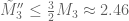 , just because
  . This is larger than the bound
  for the prism
  , which is perhaps a hopeful sign, although the upper bound here is cruder because the role of the corners of
  poking out of [0,1]^3 are ignored.
I don’t see yet though how to dissect either of the two four-dimensional candidate polytopes, namely the prism and the truncated simplex
  . (Certainly my son’s construction set is no longer of use here!)
18 December, 2013 at 8:50 am
Aubrey de Grey
Is it possible to state in purely geometrical terms what it means for a polyhedron (or polytope, but let’s start with k=3) to have polynomial moment conditions? I would like to play with possibilities for doing the chopping-up of candidate R’s systematically for k > 3, and I’m thinking that there may be alternative dissections that are superficially inferior (involve more pieces, in particular) but that turn out to be easier to generalise to larger k, but this is hard to get one’s head around without a geometrical sense of what makes a dissection admissible.
18 December, 2013 at 9:38 am
Terence Tao
The precise problem is this: given a polytope![R \subset [0,1]^k](https://s0.wp.com/latex.php?latex=R+%5Csubset+%5B0%2C1%5D%5Ek&bg=ffffff&fg=545454&s=0&c=20201002) , subdivide it into subpolytopes
, subdivide it into subpolytopes  , such that for each polytope
  and each
  , at least one of the following is true:
(1) The projection of to
to  under the operation
  of deleting the
  coordinate maps
  to a subset of
  (or equivalently,
  lies in the prism
  (which is some permutation of
 ![{\cal R}_{k-1} \times [0,1]](https://s0.wp.com/latex.php?latex=%7B%5Ccal+R%7D_%7Bk-1%7D+%5Ctimes+%5B0%2C1%5D&bg=ffffff&fg=545454&s=0&c=20201002) ); or
); or
(2) The polytope can be viewed as a region of the form
for some affine-linear functionals . In other words, all but two of the faces of
  are parallel to the
  coordinate direction. (This makes the vanishing marginal condition in the e_j direction a linear one in the coefficients of F, if F is piecewise polynomial on each of the P_i.)
In order to ensure that we recover at least in our optimisation problem, we also need to require that one of the polytopes in the partition is equal to
  . (In particular, the trivial partition in which m=1 is useless, as it only gives the trivial lower bound of 0 for M”_k.)
At present it is not obvious to me that an arbitrary polytope R actually admits such a finite subdivision; for any fixed j one can apply various slicing operations parallel to to make the subdivision good for that particular value of j, but this may introduce new problematic faces that ruin other values of j. The subdivisions I found so far were obtained by ad hoc means, and I don’t immediately see how to generalise them.
18 December, 2013 at 9:49 am
Terence Tao
Actually, it just occurred to me that we don’t, strictly speaking, need the polytopes to obey condition (2); if there are more faces that are transverse to , then we get more vanishing conditions, which reduces the number of degrees of freedom for a given degree of piecewise polynomial, but still in principle allows us to approach the optimal M”_k by using a sufficiently high degree. So one may be able to get by with a coarser partition that has more transverse faces, if the degrees of freedom tradeoff is favorable.
James: perhaps it may be a good idea to organise your code in such a way that one can easily swap in different partitions, polytopes, degree parameters, etc., to give some comparative numerical study of performance of different partitions in the k=3 case, which may give us some useful guidance before plunging into the all-important k=4 case.
17 December, 2013 at 3:15 pm
Aubrey de Grey
Many thanks James – and, in advance, for the details. In particular, can you elaborate on the basis of your remark concerning ? – I was presuming that there is no simple algorithm for dissecting
  with
with  according to Eytan’s idea, which is surely a prerequisite for making any such estimate, but maybe there is one?
17 December, 2013 at 4:53 pm
James Maynard
Aubrey: I agree there is no simple algorithm at present. The same sort of decompositions should work for , although the decomposition will probably be in many more pieces. I think it should be tedious but probably relatively straightforward to do it by hand.
My comment regarding this improvement potentially not getting all the way to was because we need an improvement of about 0.063 on the current bound for
  . When
  we appear to get an improvement of 0.072 in going from
  to
to  . My guess was that the improvement in moving from
  to
to  would decrease quite quickly in
  (as it does moving from
  to
to  ), and so the current improvement of 0.072 would probably decrease to below the required 0.063. This is just my guess though (I have no proof of this) – it would be nice if I was wrong on this front.
17 December, 2013 at 5:09 pm
Terence Tao
Well, from a volume perspective at least, has much bigger volume (
 , compared with
  for
for  and
and  for
for  ), which gives one hope. Of course, much of this extra volume is somehow “cancelled out” by the additional vanishing marginal conditions, so things are inconclusive.
This is a degenerate data point, but the improvement from M’_2 to M”_2 is precisely zero, so the improvement certainly got better going from k=2 to k=3. Perhaps going from k=3 to k=4 we still have a little bit of upward monotonicity – well, we can hope, anyway :)
18 December, 2013 at 12:19 pm
James Maynard
I’ll try to give some more details of my calculations (and hopefully if I’ve made a mistake someone will spot it). I’m not sure that I’m explaining this in the clearest language, but I hope it makes sense.
As described in Terry’s post, we are looking at polynomials supported on
  respectively.
Let’s concentrate on the calculation of , the calculations of
  being similar.
I considered the projections of onto the
  plane. For example, the projection of
  is given by
  . Based on these projections, I split the
  plane into 6 disjoint polytopes given by


 had a fixed set of the
  regions which projected to it (and those regions projected onto the whole of
  ). Since the
  regions were given by a set of linear inequalities, so too were the
  regions (and in particular they are convex).
These were formed by just splitting the projections so that each region
The point of these regions is that for in any region the integration over
  can then be written as integration over an interval. We see that the integration over
  for
for  must be zero from our marginal conditions (since
  ).
).
Over each region, we can write down the integration :
:


 over
over  correspond exactly to the vanishing conditions terry wrote above.
The regions of integration for
Thus we can perform the above integrations for with respect to
  , square, and then integrate over the regions
  . This gives our expression for
  as a quadratic form in the coefficients of
  .
.
To enforce the vanishing marginal conditions, we simply calculate the polynomials given by Terry above (i.e. the 2-variable polynomials obtained by integrating with respect to ). Each coefficient of a monomial
  gives a (homogeneous) linear constraint on our coefficients. By simply using each linear constraint to eliminate one variable at a time from the quadratic form
  , we arrive at a reduced quadratic form which satisifies all the vanishing marginal conditions. Doing the same for
  then gives us the ratio of two quadratic forms, which is our quadratic programming problem from before.
It should be relatively straightforward to modify my code so that given a decomposition into polytopes given by inequalities for linear functions
  it can calculate the quadratic form corresponding to the integration over the polytope.
18 December, 2013 at 12:43 pm
James Maynard
Also, unless I’m missing something, I think in principle there should be a fairly simple algorithm for decomposing any region given by linear inequalities to polytopes of the type we desire.
Assume we are given some region which is given by a set of linear inequalities in the variables
  . We can split this into
  subregions
  depending on which of the forms
  are greater than 1, and which are less than 1. Each such subregion will also just be given by a set of linear inequalities. We let
  be a fixed polynomial
  on each such region
  . Since we know exactly which of the functions
  are greater than 1 on
  , each region comes with a set of
  vanishing marginal conditions, where
  is the number of the
  which are greater than 1.
Each region can be further decomposed into regions
  which are of the form
  for linear functions
  . (Proof: induction on
  . Since
  is given by a set of linear inequalities, the lower and upper bounds for
  are given by the maximum and minimum of a set of linear functions in
  . For a each ordering of these functions, this gives a upper bound and lower bound for
  which is linear. Then we use the induction hypothesis, since the remaining variables are constrained only by linear inequalities).
We then decompose the projections in the coordinate of the
  regions as above (so we have regions where each region is projected to from a fixed set of the
  ). This means on each of these subregions (which are also just given by linear inequalities) the integral of
  with respect to
  is given by a finite sum of integrals of
  over intervals. Thus we can calculate all these integrals explcitly and calculate the quadratic form
  . Similarly for the other
  regions.
We still need to apply the linear constraints, but by following exactly the same method above, we can calculate the various degree polynomials corresponding to the vanishing marginals, which gives a set of homogeneous linear constraints on the coefficients of the
  . Eliminating variables from the quadratic forms then gives reduced quadratic forms satisfying the vanishing conditions.
Since everything is just given by linear constraints at each stage, everything remains convex so we avoid issues to do with a lack of convexity.
Obviously the above would give some huge number of decompositions if done directly. We can save a lot for small by using symmetry and sometimes switching the orderings of the variables to mean we only have to consider fewer regions. Thus it is probably the case that it is still better to do things by hand.
18 December, 2013 at 1:18 pm
Aubrey de Grey
Splendid! Hm, but if an economical decomposition is hard to find even for k=4, maybe it is worth seeking an algorithm to convert your decomposition into something with a more manageable number of components. The first approach that springs to mind is to do the decomposition as you describe and then iteratively examine each pair of component polytopes that share a (k-1)-dimensional polytope, to see whether their union satisfies the necessary conditions, and merge them if it does. Is there any reason why that would be expected to run into the sand unhelpfully quickly?
18 December, 2013 at 1:35 pm
James Maynard
In case my first post isn’t clear, I thought I’d try to write out explicitly what I get for some of the integrals. (Also it might make any mistakes I made clearer – there are enough terms that I can’t rule out I’ve made a small mistake somewhere).
Not assuming symmetry, I find that

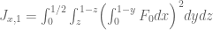

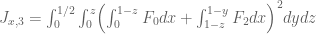


 is essentially the same, swapping all instances of
  with
with  in the integration variables and limits, and swapping the functions
  with
with  everywhere.
where
And this is subject to the three vanishing marginal conditions
The expression for
For I obtained

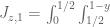

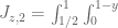
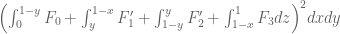


 since we are restricting to
  anyway.
where
There are no vanishing conditions for
18 December, 2013 at 4:32 pm
Pace Nielsen
James, did you get a chance to try the computation for on the new domain I described above (which Terry was kind enough to work out the linear constraints for)?
18 December, 2013 at 4:43 pm
James Maynard
I think my comments above can give a relatively straightforward decomposition of the region
![\mathcal{R}''_4=\{(x,y,z,w)\in[0,1]^4:x+y+z\leq 1\}.](https://s0.wp.com/latex.php?latex=%5Cmathcal%7BR%7D%27%27_4%3D%5C%7B%28x%2Cy%2Cz%2Cw%29%5Cin%5B0%2C1%5D%5E4%3Ax%2By%2Bz%5Cleq+1%5C%7D.&bg=ffffff&fg=545454&s=0&c=20201002)
 into 8 subregions which I’ll label
  . To ease notation let
  and similarly define
  which are the forms which are the sum of all variables except for
  or
or  respectively. Then
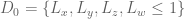


 (the subscripts are indicating which of the
  are greater than 1).
We split
and similarly for
We choose our function to be a polynomial
  of each region
  . (For the time being I won’t assume any symmetry, although this can be used to simplify things later).
To calculate :
: space into 6 subregions given by
  and all permutations of the subscripts. (For the
  regions the subsripts are intended to be ordered, whist the
  regions the subscripts are unordered). The region
  is given by

 regions.
We split the
and similarly for all other
If we restrict to , then the inner integration
  is a sum of integrals of the functions
  over intervals. For example, for
  we find
  is given by

 for any region
  . Thus we can calculate the quadratic form
  . There are no vanishing marginal restrictions here.
It is easy to write explicit limits for the integration with respect to
To calculate we follow a similar approach. We again split the
  space into regions
  etc giving the orderings of the sizes of
  . However, we further split
  into
into  and
and  depending on whether
  or
or  . For example, we obtain for

 we obtain the vanishing condition

whilst for
By symmetry, in this case we only need to consider functions for which
  for any permutation
  of
of  . This should reduce the search space significantly. For example,
  and
and  will be symmetric in
  , whilst
  will be symmetric in
  but equal to one of the other functions under transpositions of
  or
or  .
.
I haven’t had a chance to actually try to compute anything with this yet, though. I also haven’t had a chance to compute with Pace’s alternative region. (Work to do, although I’ll be busy with other things for most of tomorrow.)
16 December, 2013 at 2:32 pm
Terence Tao
I can get rid of the final error in the asymptotic lower bound for
  , thus
I’m recording a sketch of the argument below; I may give a more detailed proof for the next blog post.
The basic idea is to do a defect analysis of the upper bound . We first observe that the Cauchy-Schwarz upper bound
valid for reasonable non-negative functions , can be matched with the lower bound
for any scalar a (independent of the variable of integration). Indeed, the right-hand side can be calculated to be .
.
Now, recall that the upper bound comes from the inequality
for any , where
  and
and  is short for
  ; this comes from applying (1) with
  . Integrating this in the variables
  and then symmetrising gives the upper bound.
Now we make the usual choice of testing
where![g = G 1_{[0,T]}](https://s0.wp.com/latex.php?latex=g+%3D+G+1_%7B%5B0%2CT%5D%7D&bg=ffffff&fg=545454&s=0&c=20201002) and
and  , where
  are parameters at our disposal; a good choice here is
  and
and  for a small absolute constant
  . Applying (2) with
  , we obtain that
If we symmetrise, and let be iid random variables with law
  , where
  , then
where , and hence
where is now interpreted as
  , and the integral is interpreted as vanishing if
  is negative. One can compute that
  , and from the second moment
  if
if  is small enough, so
The integral may be bounded by the sum of
(which by convention vanishes if ) and
) and
The first term may be bounded by
For the second term, we use the identity to write this integral as
when , and
, and
when .
.
When , we crudely bound
  ,
,  to bound this integral by
  . When
  , we bound
  and
and  to bound this integral by
  . Putting all this together, we see that
where we are implicitly reducing to the event that is positive.
The second moment method shows that has mean
  and variance
  ; this makes all the error terms
  except possibly for the
  term, but this can also be made to be O(1) by an averaging argument (dilating the g’s by
  and using the pigeonhole principle).
In principle this analysis might give better numerics for the m=2 bound, but it’s a bit messy.
18 December, 2013 at 12:45 am
Andrew Granville
Terry: please can you give more details when you write “the \log \frac{c}{\theta} term … can also be made to be O(1) by an averaging argument (dilating the g’s by 1 + O(1/\log x) and using the pigeonhole principle).” ?
In my own failed efforts at proving something like this, I got stuck precisely when the range for t_k is tiny (ie reducing this term). Thanks!
18 December, 2013 at 7:42 am
Terence Tao
I wrote up some more details of the argument (with explicit error terms, which unfortunately makes things messy) at http://michaelnielsen.org/polymath1/index.php?title=Selberg_sieve_variational_problem#Lower_bounds
The averaging argument ends up being easier to run as follows: if we let be the truncation
  of a tensor product to the dilated simplex
  , then we have
We manipulate this inequality as discussed previously, converting it into an upper bound for the defect in terms of various integrals involving g and r. When one arrives at the problematic logarithmic singularity, one can then average in r (noting that the defect is independent of r).
19 December, 2013 at 12:41 pm
Eytan Paldi
Can the estimate be made effectively computable ? (or even be optimized for each given
  ?)
?)
19 December, 2013 at 2:06 pm
Terence Tao
It is certainly effective; I don’t know yet whether it is competitive with our existing bounds for m=2, but it should certainly give reasonable bounds for higher m for the first time. I’ll try to work out some more details later today..
19 December, 2013 at 6:07 pm
Terence Tao
After playing around with Maple, I was only able to get the O(1) loss in down to about 4 or 5 for medium-sized values of k, which unfortunately does not beat the current estimates for m=1,2, and gives a pretty lousy estimate for m=3; I can get
  but not much better than this. (I was hoping to recover Zhang’s original value of k=3,500,000, so that we could now stuff four primes into this tuple instead of two, but fell short of this even with our best MPZ estimate.)
I’m recording the Maple code that gave in the m=3 case below. There are three free parameters
  that one can optimise over, although I found in practice that a (somewhat artificial) constraint
  that I had to impose at some point was dominant in the sense that it set the optimal value of
  for a given c, T.
k := 10000000;

m := 3;
# These three parameters may be chosen arbitrarily
c := 1.08/log(k);
T := 0.41/log(k);
# tau := 1.14/log(k);
M0 := k*log(k)/(k-1);
g := 1/(c+(k-1)*t);
m2 := int(g*g, t=0..T );
mu := int(t*g*g, t=0..T )/m2;
sigma2 := int(t*t*g*g, t=0..T)/m2 - mu*mu;
tau := 1 - k*mu;
denominator := (1+tau/2)*(1 - (k*sigma2)/((1+tau-k*mu)^2));
a := (r - k*mu) / T;
S := r * (log((r-k*mu)/T) +(k*sigma2)/(4*a*a*T*T*log(a)) ) + r*r/(4*k*T);
Sav := int(S, r=1..1+tau, numeric)/tau;
Z3 := int( g*g*k*t*log(1+t/T), t=0..T, numeric) / m2;
W := int( g*g*log(1+tau/(k*t)), t=0..T, numeric) / m2;
X:= (log(k)/tau) * ( (1-(k-1)*mu+max(tau-c,0))^2 +(k-1)*sigma2+ c^2 );
numerator := Sav + Z3 + W*X;
Delta := (k/(k-1)) * numerator/ denominator;
# these three quantities need to be positive
evalf( 1 - k*mu - T );
evalf( 1 - k*mu - tau );
evalf(denominator);
# this is the lower bound for M_k
evalf(M0-Delta);
varpi := m/(M0-Delta) - 1/4;
delta := T * ((1/4) + varpi);
# if this is less than 1, we win
evalf(1080*varpi/13+ 330*delta/13);
19 December, 2013 at 10:47 pm
Terence Tao
I found a more efficient way to control one of the error terms (which I called Z_4 in the wiki page http://michaelnielsen.org/polymath1/index.php?title=Selberg_sieve_variational_problem#Lower_bounds ), which gets the O(1) error down to about 2 or 3, which gets the m=3 value of k down to 1,700,000. The code below also gives a value of k=38,000 for m=2 (by setting c = 1.07/log(k) and T = 0.48/log(k)); presumably a little bit more optimisation is possible.
k := 1700000;

m := 3;
# These three parameters may be chosen arbitrarily
c := 1.06/log(k);
T := 0.46/log(k);
# tau := 1.14/log(k);
M0 := k*log(k)/(k-1);
g := 1/(c+(k-1)*t);
m2 := int(g*g, t=0..T );
mu := int(t*g*g, t=0..T )/m2;
sigma2 := int(t*t*g*g, t=0..T)/m2 - mu*mu;
tau := 1 - k*mu;
denominator := (1+tau/2)*(1 - (k*sigma2)/((1+tau-k*mu)^2));
a := (r - k*mu) / T;
S := r * (log((r-k*mu)/T) +(k*sigma2)/(4*a*a*T*T*log(a)) ) + r*r/(4*k*T);
Sav := int(S, r=1..1+tau, numeric)/tau;
Z3 := int( g*g*k*t*log(1+t/T), t=0..T, numeric) / m2;
W := int( g*g*log(1+tau/(k*t)), t=0..T, numeric) / m2;
X:= (log(k)/tau) * c^2;
V := (c/m2) * int( g^2 / (2*c+(k-1)*t) , t=0..T, numeric);
U := (log(k)/c) * int( (1+u*tau - (k-1)*mu - c)^2 + sigma2, u=0..1, numeric);
numerator := Sav + Z3 + W*X + V*U;
Delta := (k/(k-1)) * numerator/ denominator;
# this needs to be positive
evalf( 1 - k*mu - T );
evalf( 1 - k*mu - tau );
# this needs to be positive too
evalf(denominator);
# this is the lower bound for M_k
evalf(M0-Delta);
varpi := m/(M0-Delta) - 1/4;
delta := T * ((1/4) + varpi);
# if this is less than 1, we win
evalf(1080*varpi/13+ 330*delta/13);
19 December, 2013 at 6:25 pm
Andrew Sutherland
Taking the first primes greater than
  gives
gives 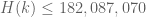 for m=3.
19 December, 2013 at 6:42 pm
Andrew Sutherland
Taking 10,000,000 consecutive primes starting with 1,040,407 gives an admissible tuple of diameter 179,933,380 for m=3.
(and 1,040,407 is the smallest prime for which this works).
20 December, 2013 at 2:32 am
Andrew Sutherland
Using the Hensley-Richards sieve for k=10,000,000 gives an admissible sequence of diameter 175,225,874 for m=3.
20 December, 2013 at 2:59 am
Andrew Sutherland
For k=1,700,000, taking the first k primes greater than k gives the bound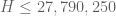 for m=3.
Taking 1,700,000 consecutive primes starting with 205,297 gives an admissible tuple with diameter 27,398,976 for m=3.
20 December, 2013 at 3:07 am
Andrew Sutherland
Using the Hensley-Richards sieve for k=1,700,000 gives and admissible tuple of diameter 26,682,014 for m=3.
20 December, 2013 at 3:16 am
Andrew Sutherland
For k=38,000 a greedy sieve yields an admissible tuple of diameter 431,682 for k=2.
20 December, 2013 at 3:38 am
Andrew Sutherland
For k=38,000 the bound on H can be improved to 430,448.
20 December, 2013 at 8:44 am
Andrew Sutherland
For m=2, k=38000 we can further improve the bound on H to 429,822.
20 December, 2013 at 8:49 am
Wouter Castryck
Terence’s maple code with the (hopefully legal?) input m := 2, c := 0.975/log(k), T := 0.97/log(k) seems to work for k = 25819. [This seems to check out – T.]
20 December, 2013 at 11:31 am
Terence Tao
Unfortunately I made a typo when entering in the formula for U; the sigma2 term should in fact be (k-1)sigma2, which makes things worse and invalidates Wouter’s optimisations – sorry about that! I was able at least to recover the k=38000 value using Wouter’s values (incidentally I have realised that it is slightly better to view c as a perturbation of 1/log(k), so I now wrote c = 1/log(k) – 0.25 / log(k)^2); similarly I can recover k=1700000 in the m=3 case by taking c = 1/log(k) – 0.07/log(k)^2 and T = 0.877/log(k)^2.
k := 38000;

m := 2;
# These three parameters may be chosen arbitrarily
c := 1/log(k) - 0.25/log(k)^2;
T := 0.97/log(k);
# tau := 1.14/log(k);
M0 := k*log(k)/(k-1);
g := 1/(c+(k-1)*t);
m2 := int(g*g, t=0..T );
mu := int(t*g*g, t=0..T )/m2;
sigma2 := int(t*t*g*g, t=0..T)/m2 - mu*mu;
tau := 1 - k*mu;
denominator := (1+tau/2)*(1 - (k*sigma2)/((1+tau-k*mu)^2));
a := (r - k*mu) / T;
S := r * (log((r-k*mu)/T) +(k*sigma2)/(4*a*a*T*T*log(a)) ) + r*r/(4*k*T);
Sav := int(S, r=1..1+tau, numeric)/tau;
Z3 := int( g*g*k*t*log(1+t/T), t=0..T, numeric) / m2;
W := int( g*g*log(1+tau/(k*t)), t=0..T, numeric) / m2;
X:= (log(k)/tau) * c^2;
V := (c/m2) * int( g^2 / (2*c+(k-1)*t) , t=0..T, numeric);
U := (log(k)/c) * int( (1+u*tau - (k-1)*mu - c)^2 + (k-1)*sigma2, u=0..1, numeric);
numerator := Sav + Z3 + W*X + V*U;
Delta := (k/(k-1)) * numerator/ denominator;
# this needs to be positive
evalf( 1 - k*mu - T );
evalf( 1 - k*mu - tau );
# this needs to be positive too
evalf(denominator);
# this is the lower bound for M_k
evalf(M0-Delta);
varpi := m/(M0-Delta) - 1/4;
delta := T * ((1/4) + varpi);
# if this is less than 1, we win
evalf(1080*varpi/13+ 330*delta/13);
20 December, 2013 at 9:02 am
Andrew Sutherland
For k=25819 we can bound H by 283,242.
20 December, 2013 at 10:11 am
Andrew Sutherland
The bound for k=25819 can be improved to 282,792.
20 December, 2013 at 10:46 am
Wouter Castryck
For m = 3, the maple code seems to prove k = 1214999 on input c = 0.995/log(k) and T = 0.877/log(k). This is probably not yet optimal.
20 December, 2013 at 10:56 am
Andrew Sutherland
For k=1700000, m=3, a greedy sieve yields an admissible tuple of diameter 25,602,510.
I can take a look at k=1214999 shortly.
20 December, 2013 at 11:03 am
Andrew Sutherland
For k=1,214,999, taking k consecutive primes starting with 157,831 gives the bound 19,152,478. Using Hensley-Richards gives 18,641,812.
20 December, 2013 at 8:17 pm
xfxie
For m=2, seems k = 36000 is valid at:
c := 0.9785232473863417/log(k);
T := 0.9205181897139338/log(k);
[Seems to check out – T.]
21 December, 2013 at 1:51 am
Andrew Sutherland
Some further improvements:
For m=2, k=38000 we can get 429,798.
For m=3,k=1,700,000 we can get 25,602,438.
21 December, 2013 at 4:32 am
Andrew Sutherland
For k=36,000 we can bound H by 405,528.
20 December, 2013 at 10:14 pm
xfxie
Here is a solution 35146, which is based on the code here (The only differences are at the four lines for the inputs k0, m, c, T).
21 December, 2013 at 4:37 am
Andrew Sutherland
For k=35146 we can bound H by 395,542.
Have you tried optimizing for m=3 (or even m=4)?
21 December, 2013 at 9:03 am
Andrew Sutherland
For m=2, k=35,146 the bound on H can be improved to 395,264.
21 December, 2013 at 10:04 am
xfxie
For k=35146 [m=2], H can be down to 395234.
21 December, 2013 at 10:34 am
Andrew Sutherland
395,178 [m=2].
21 December, 2013 at 10:20 am
xfxie
Just tried for m=3, it can be down to 1630680.
21 December, 2013 at 10:49 am
Andrew Sutherland
Thanks! Hensley-Richards then gives 25,527,718 as a bound on H.
21 December, 2013 at 6:34 pm
Andrew Sutherland
A greedy sieve brings the m=3 bound with k=1,630,680 down to 24,490,758.
21 December, 2013 at 10:31 am
xfxie
For m=4, k can be at least down to 36000000.
21 December, 2013 at 11:00 am
Andrew Sutherland
I was able to get k down to 35,127,242 for m=4, but you may be able to improve this further.
Taking the first k primes greater than k gets the bound on H down to 685,833,596 for m=4.
21 December, 2013 at 11:04 am
Andrew Sutherland
Hmm, it doesn’t seem to want to post the link. In any case, the parameters I used for m=4 to get k=35,127,242 are
c := evalf(0.9529804688/log(k));
T := evalf(0.9999999999/log(k));
21 December, 2013 at 4:23 pm
xfxie
For m=4, seems k can be decreased to 25589558.
21 December, 2013 at 6:25 pm
Andrew Sutherland
Nice improvement. Taking the first k primes greater than k=25589558 then gives the bound 491149914 on H for m=4.
Out of curiosity, have you tried m=5? It might be interesting to get a sense of how close to the asymptotic prediction we can get with explicit bounds.
21 December, 2013 at 4:51 am
Andrew Sutherland
So if I just change m to 3 in xfxie’s worksheet and then naively optimize k without changing anything else it appears that we can get 1,640,042 for m=3.
21 December, 2013 at 8:53 am
Andrew Sutherland
After fiddling with the parameters a bit, it appears that for m=3 we can get k down to 1,631,027.
Hensley-Richards then gives 25,533,684 as an upper bound on H.
21 December, 2013 at 5:04 am
Andrew Sutherland
Doing the same thing with m=4 gives k=41,862,295. Taking the first k primes greater than k gives the bound 825,018,354 on H.
18 December, 2013 at 3:46 am
Eytan Paldi
The above computation of (the operator norm of
  ) relies on the (yet unproved) assumption that it is attained as the corresponding eigenvalue for some smooth eigenfunction of
  .
.
18 December, 2013 at 8:21 am
Terence Tao
That’s a good point. Smoothness is unlikely to be an issue, because everything is at least L^2 in regularity, and all the operations involved are linear in the unknown F, so that the theory of distributions will probably be able to make all the ODE manipulations rigorous. Attainment of the minimum at an eigenfunction should be possible through calculus of variations arguments due to the strict gap (which we can prove rigorously, since
  and the explicit eigenfunction we have tells us that
  ) prevents escape to high frequencies. More precisely, let
  be a extremising sequence for the ratio
 ![[J_2^{(1)}(F_n) + J_2^{(2)}(F_n)] / I_2(F_n)](https://s0.wp.com/latex.php?latex=%5BJ_2%5E%7B%281%29%7D%28F_n%29+%2B+J_2%5E%7B%282%29%7D%28F_n%29%5D+%2F+I_2%28F_n%29&bg=ffffff&fg=545454&s=0&c=20201002) ; we can symmetrise using the parallelogram law (as mentioned in https://terrytao.wordpress.com/2013/11/19/polymath8b-bounded-intervals-with-many-primes-after-maynard/#comment-251870 ) to ensure wlog that the
; we can symmetrise using the parallelogram law (as mentioned in https://terrytao.wordpress.com/2013/11/19/polymath8b-bounded-intervals-with-many-primes-after-maynard/#comment-251870 ) to ensure wlog that the  are symmetric; we can also normalise them in L^2 and make them non-negative.
By passing to a subsequence, we can make the converge weakly in L^2. We want to upgrade this to strong convergence in L^2, so that the limit
  will be a true eigenfunction at the extremal eigenvalue
  . Because the
  have uniformly compact support and uniformly bounded in L^2, the only way in which strong convergence fails is escape of mass to high frequencies (a sort of failure of L^2 equicontinuity, in the spirit of Arzela-Ascoli). However, in the high frequency limit, at least one of the two components in
  goes to zero, and the contribution of the high frequency component is controlled by M_1, which is strictly less than M_2. This can be used to show that escape to high frequences does not occur. (There are some technical details here due to the fact that the high and low frequency components of F_n may leak outside the simplex
  , but I believe that these issues are manageable by sending the cutoff between high and low frequency slowly to infinity.)
18 December, 2013 at 10:51 am
Eytan Paldi
Concerning Aubrey’s question (on systematic dissection of ), a sufficient condition is that for each
  and each
  , the interval
for each polytope is either empty or has endpoints which are FIXED linear combinations of
  – (i.e. each endpoint belong to exactly one bounding plane of
  .)
.)
18 December, 2013 at 1:27 pm
Eytan Paldi
A possible algorithm for systematic dissection of is to check for each
  and polytope
  if every
 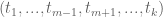 in the projection
  of
of  on the plane orthogonal to
  axis, satisfies the above condition (i.e. each endpoint of the interval
  above belongs to a FIXED bounding plane of
  . Otherwise,
  should be dissected (by appropriate planes parallel to
  axis to satisfy the above condition). I think that by repeating this dissection refinement process we get a desired dissection after finitely many steps.
18 December, 2013 at 8:22 pm
Pace Nielsen
I thought I’d give a quick update on the computational work I’ve been doing, to improve the bound we have.
I’ve tried a number of different things. One was to limit the lengths of signatures being used. It turns out that this still quickly leads to memory limitations, and also does not give good numerics in the ranges where RAM issues are gone.
Second, Frederik Ziebell sent me a very nice program to compute permutations, which is a bit slower than Mathematica, but not nearly as RAM intensive. Unfortunately, that program still eventually runs into memory issues as well!
Third, I tried pushing the degree 10 computations further, but it is clear that is the best result using the methods I’ve already tried.
Fourth, I found a computer nearby which has 64GB of RAM, and ran the program again. Surprisingly, I kept running into problems. It turns out that there is still trouble when we use signatures . In the next day or two, I will throw out this case, and maybe two other problem cases, and get a partial degree 11 result (which should push
  a bit lower).
It might be the case that I’m just not approaching the problem very well. Here is the computational hang-up:
Let be signatures (non-decreasing sequences of positive integers). Define the monomial symmetric polynomials
  as before.
We wish to compute . Once the coefficients
  are found, I put them into a look-up table and the rest of the computation does not present much difficulty.
So, the difficulty is in computing the ‘s. For anyone who wants to try to write a better algorithm than mine, a good test case is when
  . [I’m a little surprised there is not already a large look-up table of these coefficients out there (at least I can’t find one). I would think this sort of thing would be extremely useful in other contexts.]
18 December, 2013 at 9:26 pm
James Maynard
In an earlier post I think you mentioned looking at polynomials

 and
and  is a polynomial of signature
  .
.
where
Is it not possible to use these where has no 1s in its signature? This should form a basis for all symmetric polynomials, and (if I understand correctly) should avoid the RAM issues (for a bit) since you only have to add signatures which have no 1s in them, and so they should be about half the length.
This still is a bit of a hack; I’m sure there is probably a neater solution.
18 December, 2013 at 10:02 pm
Terence Tao
Perhaps one could convert between the basis of symmetrised monomials and the basis of monomials
  of the elementary symmetric polynomials (in your notation,
  where there are j 1’s)? The point is that multiplication is trivial in the latter basis (particularly from a memory standpoint, which seems to be the bottleneck). Also the operation of integrating out one of the k variables, say t_k, is not too bad in this basis, because of the recursive identities
and because t_k is being integrated from 0 to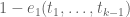 .
.
The price one pays for this of course is that integrating on the entire simplex is unpleasant in this basis, but one could now convert back to the symmetrised monomial basis in which integration is easy. It seems to be that computing the structure constants
  for
for  is relatively easy if
  is elementary, so the conversion from the monomials-of-elementary-functions basis to the symmetrised-monomials basis should be fairly straightforward. (The reverse conversion may not actually be necessary, if one stores F in the former basis rather than the latter.) In any case, these conversions should occupy significantly less memory (if one has an N-dimensional space of polynomials, any conversion matrices will take up
  memory, as opposed to the
  memory required for the multiplication structure constants
  .)
.)
For your specific example m(221111111), it looks like this polynomial is an explicit linear combination of , so
, so  is a combination of
  , and each of these should be easily expandable back into
  ‘s.
‘s.
19 December, 2013 at 1:46 pm
Pace Nielsen
James and Terry, these are both great ideas. I went with James’ idea first since it is incredibly easy to implement inside the code I have already written, and it essentially doubles the degree without much extra work. [The degree 10 case takes only about 1 minute now.]
I first accidentally ran the computation on polynomials of the form , where
  is a signature of degree
  with only *even* entries. So this set of polynomials doesn’t quite span the space of all symmetric polynomials of degree 20, but it still seems to give very good numberics (perhaps better time-wise than using the full basis–I’ll experiment with this). I obtained the lower bound
  .
.
I’ll continue running the code, lift the restriction on signatures with only even entries, and report more results tomorrow.
19 December, 2013 at 2:01 pm
Terence Tao
Ah, so we have hit , excellent! It’s remarkable how close the
  upper bound is holding up (and also reassuring that we are not contradicting that bound).
Incidentally, I changed the attribution for H(k) for small k (up to 171) on the wiki to Clark and Jarvis rather than Engelsma, as their work was earlier. (Engelsma gets optimal values up to k=342, and not necessarily optimal values up to k=800 or so.)
19 December, 2013 at 2:20 pm
Andrew Sutherland
The change in attribution makes sense. I’ll add a note to the entries in the admissible tuples database for k < 172.
If we manage to get k down to 26 we can go back further to Smith's 1957 paper.
19 December, 2013 at 2:37 pm
Eytan Paldi
This agrees with my estimate (based on linear convergence assumption) above that should be about
  , according to that assumption (with convergence rate of about
  ), the minimal
  for which $m_k > 4$ was estimated to be
  or
or  .
.
20 December, 2013 at 9:46 am
Pace Nielsen
Doing as above (considering where
where  is a signature with only even entries, and the total degree is at most 20) yields
  . [This method is definitely faster than using all monomial symmetric polynomials of a given degree, but that can still be done.] If Eytan’s predictions hold true, this will be the smallest
  value for which
  on
on  .
.
But just to give more data, here are the lower bounds on using all monomials of a given degree, for degrees
  from 1 to 14.
If any further computation is necessary, let me know.
20 December, 2013 at 9:59 am
Eytan Paldi
Since the difference should be very close to
  (i.e. very nearly
  ), we expect
  to be very close to
  – i.e. about
  .
.
20 December, 2013 at 10:42 am
Aubrey de Grey
3.987 is indeed very close to what our previous method (extrapolating differences with a 0.8 convergence rate) predicts for d=20. However, allowing d to rise to 26 appears to let M_54 creep over 4 – I trust Pace will be able to test this prediction – so it looks as though 0.8 is slightly over-pessimistic. It seems pretty certain that the corresponding series for k=53 will converge below 4, however (though of course that must also be checked).
20 December, 2013 at 11:04 am
Aubrey de Grey
Actually I retract my pessimism for k=53. Using a convergence rate of 0.8 as above, the limit of M_54 as d tends to infinity is about 4.004, but the ratio of differences for d > 10 is actually more like 0.83, which translates to a limit extremely close to 4 + 1/54, i.e. to a prediction that M_53 may creep over 4 but only for terrifyingly large d.
20 December, 2013 at 11:19 am
Aubrey de Grey
Pace – how much difference are you typically seeing for a given k and (double-digit) d between M calculated with all monomials versus only even entries? If the difference (or ratio, or some other simple function) is relatively constant, it may allow the even-entry version to act as a highly accurate estimator of what d (if any) would be needed to get M_53 > 4 using all monomials.
20 December, 2013 at 12:16 pm
Pace Nielsen
First, I should mention that using only even entries in the signature was a mistake on my part (which fortunately sped up the computation quite a bit). My intuition is that it should be better to use signatures with entries limited to for some small
  , which will keep the speed increase but not be quite so ad hoc.
Here are two data points about using limited signatures: For degree 4, , using all monomials we get
  while with restricted signatures we get
  . Similarly, in degree 10 we get the bounds
  and
and  . So it doesn’t appear that there is a significant difference in the outcome.
Regarding your pessimism, it should be kept in mind that these computations do not continue on at the same convergence rate once the degree gets to be about
  , because the monomials involved start overlapping more often. (There are fewer monomial symmetric polynomials in
  due to the lack of available variables.) So I would guess that
  is not within the realm of possibility–but I may be wrong.
I’ll see if I can’t put together some code to try degree 26 for . (Unfortunately, I do have finals to grade, and a family vacation to take this next week. So it may be a little while before it gets done.)
20 December, 2013 at 12:24 pm
Eytan Paldi
I agree with Aubrey’s conclusions. I give below more details
The last three ratios among consecutive differences are:
20 December, 2013 at 2:12 pm
Aubrey de Grey
Thank you Pace. The point about d > k/2 is well taken. The difference between the two versions of M_k for a given d is not so small, though – in fact I think it is enough, especially since it is bigger for d=10 than for d=4, that M_54 will probably not reach 4 for any d (certainly not d=26), if the even-entries version of your code is used. (That assumes that the difference is relatively independent of k, though.) Your new idea of a hybrid that includes only small odd numbers sounds ideal.
20 December, 2013 at 3:44 pm
Aubrey de Grey
Pace – before you write new code I should mention that if the convergence rate of 0.83 (rather than 0.8) is accurate, M_54 should actually reach 4 with d as small as 19.
20 December, 2013 at 3:50 pm
Aubrey de Grey
Damn, apologies – actually not until d=22.
19 December, 2013 at 4:33 am
Aubrey de Grey
The search for an ideal R has thus far proceeded by identifying extra volume that can be added to an R that is already known to be usable. I’m wondering whether there might be promise in the reciprocal option of first identifying a region that provably contains every possible R and then removing polytopes to arrive at a region that works. Would a suitable starting-point for such an approach be the union of k prisms of the form currently being investigated, i.e. a half-sized version of the region Terry describes in https://terrytao.wordpress.com/2013/12/08/polymath8b-iii-numerical-optimisation-of-the-variational-problem-and-a-search-for-new-sieves/#comment-257354 as the (Selberg-specific) minimal constraint for the sumset R+R ? (I’m actually having trouble seeing what prevents the use of that entire region itself as the maximal R, but I’m sure I’m missing something.)
19 December, 2013 at 7:58 am
Terence Tao
I had initially used this very region before realising that R+R would be too big, due to the contribution of sums r+r’ where r,r’ lie in different prisms. Pace’s symmetrised region![\{ x,y,z \in [0,1]^3: x+y+z \leq 3/2 \}](https://s0.wp.com/latex.php?latex=%5C%7B+x%2Cy%2Cz+%5Cin+%5B0%2C1%5D%5E3%3A+x%2By%2Bz+%5Cleq+3%2F2+%5C%7D&bg=ffffff&fg=545454&s=0&c=20201002) is the largest symmetric convex region available, because if
is the largest symmetric convex region available, because if  lies in a symmetric R then so does
  , and so R+R contains
  , forcing
  . There is a possibility of using a non-convex R, though one should proceed with caution in this case and recheck all the other steps of the argument.
19 December, 2013 at 8:42 am
Eytan Paldi
It seems that the generalization of Pace’s region for is
is
19 December, 2013 at 9:18 am
Eytan Paldi
For the above region we (obviously) have the upper bound

19 December, 2013 at 11:20 am
Eytan Paldi
The second inequality above is implied (of course) only for – i.e.
  .
.
19 December, 2013 at 10:56 am
Aubrey de Grey
Ah yes, of course – indeed, for k=3 it’s immediate that no R, convex or otherwise, can be bigger than half the unit cube, simply because no pair of points whose midpoint is epsilon away from (1/2,1/2,1/2) can both be in R. I’m not sure whether this generalises to larger k, though, because I’m not clear what the equivalent sumset condition is – I see various possibilities. Could you please state it explicitly?
19 December, 2013 at 11:36 am
Terence Tao
For general values of , the constraint is that R+R must lie in the set
which is the union of k prisms. For the current focus of improving the bounds on H_1 on EH, we are taking , but one could imagine that the
  case could be useful for improving the Bombieri-Vinogradov level of k (currently at 64), e.g. by using the longer prism
  , which looks like a promisingly large amount of extra room over
  .
.
20 December, 2013 at 2:46 am
Anonymous
Dear Pro.Tao,
Until now,proving H=2 is possible?Why does my intuition and mental telepathy keep feeling that 95% you can do.I’m really happy to see your answer very much.
Thank you very much,
19 December, 2013 at 2:59 pm
Eytan Paldi
The lower bound for in the wiki page should be
  (as given by James.)
[Corrected, thanks- T.]
20 December, 2013 at 8:18 am
Eytan Paldi
Currently there are several candidates for (and perhaps more future ones) for which this notation (as well as
  ) is somewhat vague – so this notation should be made clearer.
20 December, 2013 at 1:20 pm
Eytan Paldi
In the asymptotic analysis for the lower bound for in the wiki page, the integral in the numerator of the last upper bound expression for
  is not sufficiently clear.
[Clarification added -T.]
20 December, 2013 at 2:21 pm
Eytan Paldi
It seems clearer to replace by
by  in the integrand[OK, -T.].
20 December, 2013 at 2:05 pm
Polymath8b, IV: Enlarging the sieve support, more efficient numerics, and explicit asymptotics. | What's new
[…] for small values of (in particular ) or asymptotically as . The previous thread may be found here. The currently best known bounds on […]
21 December, 2013 at 9:07 am
Eytan Paldi
There are typos in the values of the upper bounds for appearing in the table in the wiki page. There is also a typo in the approximate value of
  in the last line of that page.
[Corrected, thanks – T.]
31 December, 2013 at 11:38 am
John Nicholson
Can someone explain the link of 272 to here, from the table with m=1 at: http://michaelnielsen.org/polymath1/index.php?title=Bounded_gaps_between_primes
31 December, 2013 at 12:06 pm
Andrew Sutherland
The link is to Pace Nielsen’s comment in which he notes that M_55 > 4 = 4m. By Maynard’s result (summarized above), this implies that every admissible 55-tuple has infinitely many translates that contain at least 2 primes. The bound 272 comes from the fact that there exists an admissible 55-tuple of diameter 272, e.g. this one.
2 April, 2014 at 12:30 pm
Gergely Harcos
In Section 2 of this post, should be
  (3 occurrences). Correspondingly,
 ” should be “at least
  “.
“.
in the text, “at most
[Corrected, thanks – T.]