Polymath8b, VI: A low dimensional variational problem

17 January, 2014 in math.CA, polymath | Tags: polymath8 | by Terence Tao

This is the sixth thread for the Polymath8b project to obtain new bounds for the quantity

$\displaystyle H_m := \liminf_{n \rightarrow\infty} (p_{n+m} - p_n),$

either for small values of ${m}$ (in particular ${m=1,2}$ ) or asymptotically as ${m \rightarrow \infty}$ . The previous thread may be found here. The currently best known bounds on ${H_m}$ can be found at the wiki page (which has recently returned to full functionality, after a partial outage).

The current focus is on improving the upper bound on ${H_1}$ under the assumption of the generalised Elliott-Halberstam conjecture (GEH) from ${H_1 \leq 8}$ to ${H_1 \leq 6}$ , which looks to be the limit of the method (see this previous comment for a semi-rigorous reason as to why ${H_1 \leq 4}$ is not possible with this method). With the most general Selberg sieve available, the problem reduces to the following three-dimensional variational one:

Problem 1 Does there exist a (not necessarily convex) polytope ${R \subset [0,1]^3}$ with quantities ${0 \leq \varepsilon_1,\varepsilon_2,\varepsilon_3 \leq 1}$ , and a non-trivial square-integrable function ${F: {\bf R}^3 \rightarrow {\bf R}}$ supported on ${R}$ such that

${R + R \subset \{ (x,y,z) \in [0,2]^3: \min(x+y,y+z,z+x) \leq 2 \},}$

${\int_0^\infty F(x,y,z)\ dx = 0}$ when ${y+z \geq 1+\varepsilon_1}$ ;

${\int_0^\infty F(x,y,z)\ dy = 0}$ when ${x+z \geq 1+\varepsilon_2}$ ;

${\int_0^\infty F(x,y,z)\ dz = 0}$ when ${x+y \geq 1+\varepsilon_3}$ ;

and such that we have the inequality

$\displaystyle \int_{y+z \leq 1-\varepsilon_1} (\int_{\bf R} F(x,y,z)\ dx)^2\ dy dz$

$\displaystyle + \int_{z+x \leq 1-\varepsilon_2} (\int_{\bf R} F(x,y,z)\ dy)^2\ dz dx$

$\displaystyle + \int_{x+y \leq 1-\varepsilon_3} (\int_{\bf R} F(x,y,z)\ dz)^2\ dx dy$

$\displaystyle > 2 \int_R F(x,y,z)^2\ dx dy dz?$

(Initially it was assumed that ${R}$ was convex, but we have now realised that this is not necessary.)

An affirmative answer to this question will imply ${H_1 \leq 6}$ on GEH. We are “within almost two percent” of this claim; we cannot quite reach ${2}$ yet, but have got as far as ${1.959633}$ . However, we have not yet fully optimised ${F}$ in the above problem.

The most promising route so far is to take the symmetric polytope

$\displaystyle R = \{ (x,y,z) \in [0,1]^3: x+y+z \leq 3/2 \}$

with ${F}$ symmetric as well, and ${\varepsilon_1=\varepsilon_2=\varepsilon_3=\varepsilon}$ (we suspect that the optimal ${\varepsilon}$ will be roughly ${1/6}$ ). (However, it is certainly worth also taking a look at easier model problems, such as the polytope ${{\cal R}'_3 := \{ (x,y,z) \in [0,1]^3: x+y,y+z,z+x \leq 1\}}$ , which has no vanishing marginal conditions to contend with; more recently we have been looking at the non-convex polytope ${R = \{x+y,x+z \leq 1 \} \cup \{ x+y,y+z \leq 1 \} \cup \{ x+z,y+z \leq 1\}}$ .) Some further details of this particular case are given below the fold.

There should still be some progress to be made in the other regimes of interest – the unconditional bound on ${H_1}$ (currently at ${270}$ ), and on any further progress in asymptotic bounds for ${H_m}$ for larger ${m}$ – but the current focus is certainly on the bound on ${H_1}$ on GEH, as we seem to be tantalisingly close to an optimal result here.

— 1. Analysis of the symmetric polytope —

In the symmetric situation described above, we have a single vanishing marginal condition

${\int_0^{3/2-x-y} F(x,y,z)\ dz = 0}$ when ${(x,y) \in [0,1]^2}$ is such that ${1+\varepsilon_3 \leq x+y \leq 3/2}$

and the inequality we wish to prove is that

$\displaystyle 3\int_{x+y \leq 1-\varepsilon} (\int_0^{\min(1,3/2-x-y)} F(x,y,z)\ dz)^2\ dx dy$

$\displaystyle > 2 \int_R F(x,y,z)^2\ dx dy dz.$

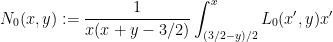
A routine calculus of variations computation, using Lagrange multipliers, tells us that the extremal ${F}$ should take the form

$\displaystyle F(x,y,z) = G(x,y) + G(y,z) + G(z,x) \ \ \ \ \ (1)$

where ${G}$ is symmetric and supported the disconnected set ${T_0 \cup T_1}$ , where ${T_0}$ is the triangle

$\displaystyle T_0 := \{ (x,y) \in [0,1]^2: x+y \leq 1-\varepsilon\}$

and ${T_1}$ is the trapezoid

$\displaystyle T_1 := \{ (x,y) \in [0,1]^2: 1+\varepsilon \leq x+y \leq 3/2 \}.$

(Strictly speaking, we have not established that an extremiser actually exists, but for the purposes of numerics it seems to be reasonable to proceed as if an extremiser does exist.) One also has the eigenfunction equation

$\displaystyle (M''_{3,\varepsilon,1})^{-1} \int_0^{\min(1,3/2-x-y)} F(x,y,z)\ dz = G(x,y)$

whenever ${(x,y) \in [0,1]^2}$ is such that ${x+y \leq 1-\varepsilon}$ , where ${M''_{3,\varepsilon,1}}$ is the quantity that we are trying to push above ${2}$ . It seems that this eigenfunction equation should indicate where exactly we expect the singularities of ${F}$ and ${G}$ to lie, and how bad they will be (our best guess right now is that the extremiser is continuous but not differentiable at certain points), but this has not yet been fully analysed.

If we use the ansatz (1), we arrive at a moderately complicated variational problem involving one unknown symmetric function ${G(x,y)}$ , which is constrained to be supported in ${T_0 \cup T_1}$ and obeys the vanishing marginal condition

$\displaystyle \int_0^{3/2-x-y} (G(x,y) + G(y,z) + G(z,x))\ dz = 0$

whenever ${(x,y)}$ lies in ${T_1}$ . If we let ${G_0, G_1}$ be the restrictions of ${G}$ to ${T_0,T_1}$ respectively (so that ${G = G_0 + G_1}$ ), this constraint becomes

$\displaystyle (3/2-x-y) G_1(x,y) + H_0(x,y) + H_1(x,y) + H_0(y,x) + H_1(y,x) = 0$

where

$\displaystyle H_0(x,y) := \int_{0 \leq z \leq \min(3/2-x-y,1-\varepsilon-y)} G_0(y,z)\ dz$

and

$\displaystyle H_1(x,y) := \int_{1+\varepsilon-y \leq z \leq 3/2-x-y} G_1(y,z)\ dz.$

This equation can be used to solve for ${G_1}$ in terms of ${G_0}$ , thus reducing to a variational problem for an unconstrained function ${G_0}$ on the triangle ${T_0}$ . In the hexagonal region

$\displaystyle \{ (x,y) \in T_1: x, y \geq 1/2 - \varepsilon \}$

the functions ${H_1(x,y), H_1(y,x)}$ vanish, and we simply have

$\displaystyle G_1(x,y) = -\frac{H_0(x,y) + H_0(y,x)}{3/2-x-y}$

(note that ${H_0}$ vanishes at the boundary ${x+y=3/2}$ , so there is no singularity here). If ${\varepsilon \geq 1/4}$ , this covers all of ${T_1}$ , and completes the reduction to a variational problem for ${G_0}$ . We do not believe this range to be the optimal value for ${\varepsilon}$ , but might be worth considering as a warmup.

Now suppose ${\varepsilon < 1/4}$ . In the triangular region

$\displaystyle \{ (x,y) \in T_1: x \leq 1/2-\varepsilon\} \ \ \ \ \ (2)$

(bounded by the vertices ${(\varepsilon,1)}$ , ${(1/2-\varepsilon,1)}$ , ${(1/2-\varepsilon,1/2+2\varepsilon)}$ ) we have vanishing of ${H_1(y,x)}$ but not ${H_1(x,y)}$ , leading to the equation

$\displaystyle (3/2-x-y) G_1(x,y) + H_0(x,y) + H_0(y,x) + \int_{1+\varepsilon-y}^{3/2-x-y} G_1(z,y)\ dz = 0. \ \ \ \ \ (3)$

To solve this equation, we first differentiate it in ${x}$ to obtain

$\displaystyle (3/2-x-y) \partial_x G_1(x,y) - G_1(x,y) + \partial_x H_0(x,y) + \partial_x H_0(y,x)$

$\displaystyle - G_1(3/2-x-y,y) = 0,$

so if we define

$\displaystyle K_1(x,y) := G_1(x,y) + G_1(3/2-x-y,y)$

and

$\displaystyle L_0(x,y) := \partial_x H_0(x,y) + \partial_x H_0(y,x)$

then

$\displaystyle \partial_x G_1(x,y) = \frac{K_1(x,y)}{3/2-x-y} - \frac{L_0(x,y)}{3/2-x-y} \ \ \ \ \ (4)$

and thus by the substitution ${x \mapsto 3/2-x-y}$ (which preserves the triangle (2), as well as ${K}$ )

$\displaystyle -\partial_x G_1(3/2-x-y,y) = \frac{K_1(x,y)}{x} - \frac{L_0(3/2-x-y,y)}{x}$

and so on subtracting

$\displaystyle \partial_x K_1(x,y) = K_1(x,y) (\frac{1}{3/2-x-y} - \frac{1}{x}) - \frac{L_0(x,y)}{3/2-x-y}$

$\displaystyle + \frac{L_0(3/2-x-y,y)}{x};$

multiplying by ${x (x+y-3/2)}$ and rearranging, this becomes

$\displaystyle \partial_x ( x (x+y-3/2) K_1(x,y) ) = L_0(x,y) x$

$\displaystyle + L_0(3/2-x-y,y) (x+y-3/2),$

so we have

$\displaystyle K_1(x,y) = N_0(x,y) + C_1(y) (3/2-y) ( \frac{1}{x} + \frac{1}{3/2-x-y} )$

for some function ${C_1(y)}$ , where

$\displaystyle N_0(x,y) := \frac{1}{x(x+y-3/2)} \int_{(3/2-y)/2}^x L_0(x',y) x'$

$\displaystyle + L_0(3/2-x'-y,y) (x'+y-3/2)\ dx',$

where we are using the signed integral, thus ${\int_b^a = -\int_a^b}$ when ${a>b}$ . Note that when ${x = (3/2-y)/2}$ , ${N_0(x,y)}$ vanishes and ${K_1(x,y) = 2 G_1(x,y)}$ , and so

$\displaystyle G_1( (3/2-y)/2, y ) = 2 C_1(y).$

Meanwhile, from (4) we have

$\displaystyle \partial_x G_1(x,y) = \frac{N_0(x,y)-L_0(x,y)}{3/2-x-y} + C_1(y) \frac{(3/2-y)}{(3/2-x-y)^2}$

$\displaystyle + C_1(y) (\frac{1}{x} + \frac{1}{3/2-x-y})$

and so

$\displaystyle G_1(x,y) = P_0(x,y) + C_1(y) ( \frac{3/2-y}{3/2-x-y} + \log \frac{x}{3/2-x-y} )$

where

$\displaystyle P_0(x,y) := \int_{(3/2-y)/2}^x \frac{N_0(x',y)-L_0(x',y)}{3/2-x'-y}\ dx'.$

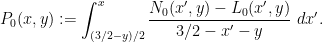
On the other hand, from (3) with ${x=1/2-\varepsilon}$ one has

$\displaystyle (1+\varepsilon-y) G_1(1/2-\varepsilon,y) + H_0(1/2-\varepsilon,y) + H_0(y,1/2-\varepsilon) = 0$

and so we may solve for ${C_1}$ as

$\displaystyle C_1(y) = - \frac{ \frac{1}{1+\varepsilon-y} (H_0(1/2-\varepsilon,y) + H_0(y,1/2-\varepsilon)) + P_0(1/2-\varepsilon,y)}{ \frac{3/2-y}{1+\varepsilon-y} + \log \frac{1/2-\varepsilon}{1+\varepsilon-y} }$

which gives an explicit (but messy) formula for ${G_1}$ in terms of ${G_0}$ in the triangle (2); by symmetry one also describes ${G_1}$ in the triangle

$\displaystyle \{ (x,y) \in T_1: y \leq 1/2-\varepsilon \},$

and this completes the description of ${G_1}$ in terms of ${G_0}$ . (The exact description is, however, rather messy, in particular requiring a certain amount of integration; it is not clear whether we should actually use it for the purposes of efficient numerics.)

104 comments

Comments feed for this article

17 January, 2014 at 3:54 pm

Eytan Paldi

In problem 1, $F$ should be in $L^2(R)$ with positive norm, and in the definition of $R$ the maximum should be $\leq 2$ .

[Corrected, thanks – although the constraint $R+R \subset [0,2]^3$ actually already forces $R \subset [0,1]^3$ . -T.]

17 January, 2014 at 4:27 pm

Eytan Paldi

The maximum (in the def. of $R$ ) should be corrected to $\leq 2$ (instead of $\geq 2$ ).
And three closing parentheses are missing.

[Corrected, although I don’t see where the three missing closing parentheses are. -T.]

17 January, 2014 at 5:50 pm

Eytan Paldi

I’m sorry (no need for closing parentheses.)

17 January, 2014 at 4:45 pm

Eytan Paldi

It seems that condition (4) in the previous thread is that the minimum is $< 2$ .

[Corrected – T.]

17 January, 2014 at 4:02 pm

Anonymous

Just before “1. Analysis of the symmetric polytope”: 272 –> 270.

[Corrected, thanks -T.]

17 January, 2014 at 4:06 pm

Anonymous

The very last word: “numericss” –> “numerics”

[Corrected, thanks -T.]

17 January, 2014 at 6:22 pm

Eytan Paldi

It seems that in the eigenfunction equation above, $M''_{3, \epsilon, 1}$ should be on the RHS.

[Corrected, thanks – T.]

18 January, 2014 at 9:23 am

Eytan Paldi

It seems that the LHS should be without the factor 3.

[Corrected, thanks – T.]

17 January, 2014 at 6:38 pm

Aubrey de Grey

Two quick questions relating to loose ends from the previous thread:

1) Can I just clarify: is it still believed that H_1 could be reduced from 8 to 6 on GEH if M”_4 could be pushed to a point that allows “n,n+8 both prime” to be excluded (estimated as 2.35), or is there now a variant of the argument for k=3, H_1=4 which precludes that? I ask only because this avenue for progress is strangely unmentioned in the new post.

2) While the focus remains on k=3 it seems worthwhile to maintain some awareness of the potential for ideas currently in play to translate to the unconditional setting as and when attention returns to it. In particular, the original mention of converting F(x,y,z) to G(x,y) noted the computational efficiency advantage, so it would be valuable to understand whether a corresponding conversion can be performed for larger k. If it can, does it also preserve the ability to avoid partitioning (at the cost of looking at a reduced range of possible F’s) that was mentioned in the thread before last?

17 January, 2014 at 8:19 pm

Terence Tao

I don’t see any strong barrier to the k=4 approach to $H_1 \leq 6$ , except for the purely numerical one that we would have to make a much larger improvement in the M_4 statistic to reach this than we would for the M_3 statistic. (Note that 2.35 is only a heuristic computation; in practice, we would probably have to be more efficient still than this.)

I’m hoping that by playing around with enough variants of the k=3 problem, we will naturally discover efficient ways to do slightly higher values of k (4 or 5, for instance), and can maybe start extrapolating how much gain one could get from various tricks in higher k. I suspect though that most of these gains decay rather fast in k, though if we become better at optimising on the truncated simplex, then we could finally use some of the Polymath8a results, which so far have only been used for m >= 2.

18 January, 2014 at 7:54 am

Pace Nielsen

Aubrey, as you pointed out in the previous thread, I was being more than a little optimistic that we could reach 2.35. It’s still worthwhile to see what happens (if we can’t make the k=3 case work), but now that I’ve thought about it a bit more, getting to 2.35 seems like a long shot.

18 January, 2014 at 2:38 am

Eytan Paldi

Three lines above (1), the LHS should be multiplied by 3.

[Corrected, thanks – T.]

18 January, 2014 at 4:00 am

Eytan Paldi

The exact expression of $G_1$ is (at least) useful by providing more detailed information on the possible locations (and types) of its singularities in $T_1$ (assuming certain regularity properties of $G_0$ in $T_0$ ).
$G_0, G_1$ may be approximated by piecewise polynomials (using polygonal partition adapted to the above information on the possible locations of singularities).

18 January, 2014 at 8:39 am

Anonymous

I cannot see the last part of the inequality just above (1); maybe “ $> 2 \int_R F(x,y,z)^2 \,dx\,dy\,dz.$ ” should be put on a new line.

[Corrected, thanks – T.]

18 January, 2014 at 10:09 am

Aubrey de Grey

I’ve been reviewing Pace’s data from the past week to see whether there is any anomalous pattern.

First, Pace: I’m uncertain which polytope you were using for the data you reported in https://terrytao.wordpress.com/2014/01/08/polymath8b-v-stretching-the-sieve-support-further/#comment-264511 and https://terrytao.wordpress.com/2014/01/08/polymath8b-v-stretching-the-sieve-support-further/#comment-264615. In each case, was it R’, the prism or the symmetric half-cube? Your description in 264511 looks like the prism, but you referred to it as M’ and then in 264615 as “the symmetric case” so I wanted to check. In particular, it would be good to clarify whether the symmetric half-cube behaves like R’ in gaining 2/3 as much from using epsilon,epsilon,0 as from using eps,eps,eps.

My main focus is the fact (already pointed out, of course) that the best M value we have for the symmetric half-cube (using three equal epsilons) is only 0.007 greater than for R’ (1.9596 versus 1.9527). This is an order of magnitude less than the difference of 0.06 without epsilons (1.9026 versus 1.8429). I think this suggests that the putative inefficiency of partitioning in the presence of epsilons is hurting much more in the non-R’ polytopes within the symmetric half-cube than it is within R’. Is that a reasonable interpretation? If so, then maybe one idea would be to do Terry’s variable-degree trick in reverse, i.e. to look at high degree for a subset of the non-R’ polytopes (just the A’s, or just the B’s, etc) rather than for R’ itself. Worth a try?

18 January, 2014 at 1:55 pm

Pace Nielsen

The polytope was the one exactly described in comment 264511. It is the prism with cut-offs when $y+z\leq 1+\epsilon_1$ and $x+z\leq 1+\epsilon_2$ .

I’m not sure when I’ll have time to get back to these computations. One of my coauthors sent me a draft of our paper, and I’ll be focused on that for the next few days. If you want to give your variable-degree idea a try, you are welcome to the code. Just email me on Tuesday and I’ll send the mathematica notebook to you.

18 January, 2014 at 8:12 pm

Aubrey de Grey

Many thanks Pace – OK, so it’s definitely R’ with two equal epsilons added, so we don’t yet have data on the symmetric half-cube with two equal epsilons added. Please do send me the code (aubrey@sens.org) – thanks! – though I too am overstretched and don’t promise to have the time, especially since I am an extreme Mathematica novice.

19 January, 2014 at 10:47 am

Aubrey de Grey

OK, a very brief fiddle with Pace’s code (on the prism, which is the code he had to hand at home) makes this idea look unpromising – increasing the degree to 6 for just one category of component polytopes does not raise M” by more than 0.001 in any case. (I may have done it wrongly, however, because sometimes M” actually fell and because I received some alerts about the matrix inversion being “badly conditioned”.) If this is correct and applies also to the symmetric half-cube, perhaps the takeaway is that the partitioning is just losing a lot in all cases examined so far – which concords with Terry’s suggestion that there are loads of singularities in G_0. As a first data point I checked the prism with epsilon set to 0.25 and found that M” falls by only about 0.017 relative to that for the optimal epsilon of 0.157 found earlier by Pace, so it indeed seems useful to explore the “warmup” option Terry mentioned above (in which, if I understand Terry’s earlier comment about the likely locations of singularities, T_0 will need only a not-very-scary four partitions).

19 January, 2014 at 12:45 pm

Eytan Paldi

A more efficient and numerically stable evaluation of any M-value is to represent it as the largest eigenvalue of a linear matrix pencil $(A, B)$ ( see the application section in the wikipedia article on matrix pencil) for which there is an efficient and numerically stable algorithm (without matrix inversion!)

20 January, 2014 at 8:03 am

Aubrey de Grey

Interesting! When Pace was working on k=54 or so he mentioned that the inversion step was causing RAM issues, so this could be a valuable new tool. (Then again, he did note at the same time that there were also RAM issues when finding the largest eigenvector of similarly sized matrices, so maybe he’s already doing this when needed.)

20 January, 2014 at 8:51 am

Eytan Paldi

This can be implemented in mathematica, see e.g.

http://reference.wolfram.com/legacy/applications/anm/GeneralizedEigenvalueProblem/9.1.html

20 January, 2014 at 10:41 am

Aubrey de Grey

I’ve now received Pace’s code for the symmetric half-cube and also (thanks to a suggestion from him) eliminated the alerts I mentioned. As with the prism, it turns out that the benefits to M” from increasing the degree for just one category of partition is much less for any of the non-R’ categories than it is for R’ itself (but it is always positive, so I’m pretty sure I did it correctly this time). A new partitioning that respects singularities seems, therefore, to be an absolute requirement for meaningful further progress.

18 January, 2014 at 2:02 pm

Eytan Paldi

Since the explicit (somewhat messy) expression for $G_1$ depends linearly on $G_0$ , another possible approach is to use a basis of symmetrical polynomials to approximate $G_0$ on $T_0$ with a corresponding basis of functions (derived by the above explicit expression) for $G_1$ on $T_1$ . If the basis of functions for $G_1$ is not “too complicated”, the needed two dimensional integrals representing the elements of the matrices for the unconstrained optimization program may be computed sufficiently accurately.

19 January, 2014 at 9:10 am

Eytan Paldi

In the representation of the vanishing marginal condition using (1), the integrand should be inside parentheses.

[Edited, thanks – T.]

19 January, 2014 at 2:44 pm

Aubrey de Grey

On another topic: just before Christmas (https://terrytao.wordpress.com/2013/12/20/polymath8b-iv-enlarging-the-sieve-support-more-efficient-numerics-and-explicit-asymptotics/#comment-258871) Terry improved the asymptotic bounds on H_m in the setting of the MPZ estimates, but I don’t think there was any mention that this was taken through into a modification of the Maple code that xfxie was using to identify minimal k’s. Is any such modification needed? If so, and if it wasn’t done yet, maybe it would give xfxie and Drew something to do while the focus is on k=3 :-)

19 January, 2014 at 2:51 pm

Polymath 9 | Euclidean Ramsey Theory

[…] is a post discussing this. Meanwhile Polymath 8 has spawned a new project Polymath 8b. https://terrytao.wordpress.com/2014/01/17/polymath8b-vi-a-low-dimensional-variational-problem/ is the latest post of this […]

20 January, 2014 at 1:37 am

Eytan Paldi

In the simple expression for $G_1(x, y)$ (six lines above (2)), the RHS should be with a minus sign.

[Corrected, thanks – T.]

20 January, 2014 at 11:12 am

Eytan Paldi

The exact value of $M''_{3, \epsilon, 1}$ for $\epsilon \in (1/2, 1)$ :

In this (simplest) case, the set $T_1$ is empty and therefore $G=G_0$ is supported on $T_0$ . Since in this case $\min (1, 3/2 - x - y) = 1$ , it follows (assuming the existence of an optimal $F$ ) from the eigenvalue equation and the representation (1) that

$\lambda G(x, y) = G(x, y) + H(x) + H(y)$ , $(x, y) \in T_0$

where $\lambda := M''_{3, \epsilon, 1}$ and

$H(x) := \int_0^1 G(x, z) dz$ is supported on $[0, 1 - \epsilon]$ . Hence

$(\lambda - 1)H(x) = \int_0^{1-\epsilon} [H(x)+H(z)]dz$ . Showing that $H$

is a constant supported on $[0, 1 - \epsilon]$ . We may normalize it as

$H(x) := 1_{[0, 1 - \epsilon]}(x)$ . Hence

$(\lambda - 1) = 2(1 - \epsilon)$ , implying

$M''_{3, \epsilon, 1} = 3 - 2 \epsilon$ .

Remark: This expression seems to hold in the limiting case $\epsilon = 1/2$ (since in this case the set $T_1$ still has zero area measure).

20 January, 2014 at 12:10 pm

Aubrey de Grey

Splendid! If this is confirmed, it would be positively cruel if an epsilon slightly less than 1/2 were not a win…

20 January, 2014 at 12:18 pm

Terence Tao

Unfortunately I think the integral $\int_0^{1-\varepsilon} [H(x)+H(z)]\ dz$ should in fact be $\int_0^{1-\varepsilon-x} [H(x)+H(z)]\ dz$ , as G(x,z) is supported on the region $z \leq 1-\varepsilon-x$ . This equation should still be exactly solvable for H, and hence for G and F (by an analysis similar to that providing the exact solution for M_2, or for solving for G_1 in terms of G_0) but it is going to lead to a messier answer than $3-2\varepsilon$ , I’m afraid.

20 January, 2014 at 12:53 pm

Eytan Paldi

I see the problem: The first formula expressing $G(x, y)$ in terms of $H(x), H(y)$ is known to hold for $(x, y) \in T_0$ (but not necessarily on $[0, 1-\epsilon]^2$ ).

20 January, 2014 at 1:41 pm

Eytan Paldi

Yes. I almost have the solution (H satisfies a very simple second order equation!)

20 January, 2014 at 9:02 pm

Eytan Paldi

The corrected derivation of $M''_{3, \epsilon, 1}$ is

1. The corrected equation for $H(x)$ follows by integrating the representation (on $T_0$ ) of $G(x, z)$ with respect to $z$ over $[0, 1-\epsilon -x]$ (for which the representation holds!). This gives

(*) $(\lambda - 1)H(x) = (1-\epsilon -x)H(x) + \int_0^{1-\epsilon - x} H(z) dz$

This is the corrected equation for $H$ on $[0, 1-\epsilon]$ .

2. Assuming $H$ to be sufficiently smooth, we have

(1) $(\lambda - 1)H'(x) = -H(x)+(1-\epsilon-x)H'(x) + H(1-\epsilon-x)$

By reflection ( $1- \epsilon -x$ instead of $x$ ) we have

(1′) $(\lambda-1)H'(1-\epsilon -x)=-H(1-\epsilon -x)+x H'(1-\epsilon -x)+H(x)$

Now we use (1) to express

(2) $H(1- \epsilon -x) = (\lambda -2 + \epsilon +x) H'(x) + H(x)$

So by taking derivatives

(2′) $H'(1-\epsilon - x) = -2 H'(x) -(\lambda - 2 +\epsilon +x)H''(x)$

Substitution of (2) and (2′) in (1′) gives

$(x+1-\lambda)(x+\lambda +\epsilon -2) H''(x)+(3 x +\epsilon -\lambda)H'(x) = 0$

Implying that the logarithmic derivative of $H'(x)$ is

$-1/(x+1-\lambda) - 2/(x+\lambda +\epsilon -2)$

Giving (the normalized)

(3) $H'(x) = 1/[(x+1-\lambda)(x+\lambda +\epsilon -2)^2]$

Which gives

(4) $H(x) = K^{-2}[\log |\frac{x-a}{x+b}| + \frac{K}{x+b}] + C$

Where $K=2 \lambda +\epsilon -3, a=\lambda -1, b= \lambda +\epsilon -2$ and $C$ is an integration constant (to be determined with $\lambda$ ).

3. In order to determine $C$ and $\lambda$ we need two boundary conditions. First, observe that (*) implies

(i) $(\lambda -1)H(1-\epsilon) = 0$

Assuming $\lambda \neq 1$ , we have

(i)’ $H(1-\epsilon) = 0$ , implying

$C = - K^{-2}[log |\frac{2-\epsilon -\lambda}{\lambda -1}| +K/(\lambda -1)]$

In order to determine $\lambda$ , we need another boundary condition.

By (2) and (i)’ we have $H(0) = (\lambda -1)H'(1-\epsilon)$

Therefore by (3)

(ii)’ $H(0) = \frac{1}{(\lambda - 1)(2-\lambda - \epsilon)}$

Using this in (4), we see that $\lambda$ satisfies

(5) $(2 \lambda +\epsilon -3)^2 = 2(\lambda -1)(2-\lambda -\epsilon)\log |\frac{\lambda -1}{2-\lambda -\epsilon}| -(1-\epsilon)(2\lambda +\epsilon-3)$

Therefore $M''_{3, \epsilon, 1}$ should be the largest positive root of (5).

Remark:

Note that since the argument of the logarithm in the above expression for $C$ should be nonzero and finite, this is equivalent that $H(0)$ should not vanish. In particular, the assumption $H(0) >0$ implies the simple inequality

$1 < \lambda < 2-\epsilon$

20 January, 2014 at 9:22 pm

Terence Tao

Thanks for this! One could use this exact solution to benchmark the convergence of the numerics (with or without partitioning, using G instead of F, etc.); even in this simple regime $\varepsilon > 1/2$ in which many of the polytopes have disappeared, it appears that G still has a jump discontinuity at $x+y=1-\varepsilon$ , leading to corresponding discontinuities for F which require some partitioning in order to be able to efficiently work around. (Conversely, one can use the numerics to confirm the correctness of the exact solution.)

It also occurs to me that if we work in the two-dimensional G formulation rather than the three-dimensional F formulation, then we can make plots of G that will help strengthen our intuition as to how the singularities are distributed.

20 January, 2014 at 10:05 pm

Pace Nielsen

I think there is something wrong here. Graphically, the largest positive root of (5), in the range $1< \lambda < 2-\varepsilon$ , appears to always be $\lambda=3/2-\varepsilon/2$ . Taking $\varepsilon=1/2$ , we are then getting $M''_{3,1/2,1}=1.25$ (and in that special case, this is indeed the largest root). But numerically I'm getting $M''_{3,1/2,1}\geq 1.69296...$ . Hopefully I'm not missing something simple.

20 January, 2014 at 11:10 pm

Eytan Paldi

Interestingly, it is easy to verify that the root is exactly $(3-\epsilon)/2$ .
(In fact all the three terms are zero!) I’ll check again the derivation.

20 January, 2014 at 11:37 pm

Eytan Paldi

For this $\lambda$ it follows that $H$ vanish identically! (i.e. it is the trivial solution!). If the derivation is correct than something must be wrong with the assumptions (e.g. existence of a smooth optimal solution.)

21 January, 2014 at 7:55 am

Eytan Paldi

You are right! In fact, I just found an easy proof that

$M''_{3, \epsilon, 1} = 1+(1-\epsilon) M_2$ for $\epsilon \in [1/2, 1)$

This connection to the constant $M_2$ is very interesting!

Concerning your example, using $M_2 = 1.38593...$ , we get

$M_{3, 1/2, 1} = 1 + \frac{1}{2} M_2 = 1.6929...$

I’ll send the details in my next message.

21 January, 2014 at 8:46 am

Aubrey de Grey

Great work Eytan! Even though 1.69 is a long way from 2, I’m wondering whether this finding could help to indicate which half-cube is really the best. Pace: do you numerically get this same value for both the prism and the symmetric half-cube? (I’m presuming that I can’t check this myself with the code you sent me because a different partitioning is needed for epsilon that large.) If the prism leads to a smaller M” for epsilon=1/2, I think that would constitute a significant strengthening of the evidence that there is no need to consider any half-cube other than the symmetric one from now on.

21 January, 2014 at 11:53 am

Eytan Paldi

Derivation of $M''_{3, \epsilon, 1}$ for $\epsilon \in (1/2, 1)$

Observe that $G$ is supported on $T_0 = (1-\epsilon) \mathcal R_2$ .
Therefore it seems reasonable that there is some (scaling) connection to the $M_2$ variational problem. Recall (for comparison purpose) that

1. In the $M_2$ problem, the eigenvalue equation was

(1) $M_2 f(x) = (1-x) f(x) + \int_0^{1-x} f(y) d y$ , $x \in [0, 1]$

with the solution

(2) $f(x) = \frac{2 M_2 -1}{M_2 -1+x} + \log \frac{M_2 -x}{M_2 -1+x}$

2. For the current problem, the eigenvalue equation is (see previous comment)

(*) $(\lambda -1)H(x) = (1-\epsilon - x)H(x)+\int_0^{1-\epsilon-x}H(y)d y$

where $H$ is now supported on $[0, 1-\epsilon]$ .

Let $H$ be a solution of (*), than (by a change of variables) we have the equivalent form (with $x=(1-\epsilon)x' , y= (1-\epsilon)y'$ )

(*)’ $(\lambda -1)\phi(x') = (1-\epsilon)[(1-x')\phi(x')+\int_0^{1-x'} \phi(y')d y']$

where $\phi(x') := H((1-\epsilon)x')$ is supported on $[0, 1]$ .

By comparing (*)’ to (1), it follows that

$(\lambda -1)/ (1-\epsilon) = M_2$ , hence

(3) $M''_{3,\epsilon, 1} = \lambda = 1+ (1-\epsilon) M_2$

Remark: From this comparison, it follows that the solution $H$ to (*) is given by

(4) $H(x) = f(x/(1-\epsilon)) , x \in [0, 1-\epsilon]$

where $f(x)$ is given by (2).

20 January, 2014 at 3:47 pm

Eytan Paldi

I found $H(x)$ to be an explicit fourth degree polynomial on $[0, 1 - \epsilon]$ and $M''_{3, \epsilon, 1}$ was found to be the largest positive root of an explicit fourth order polynomial. I’ll give the details in my next comment.

20 January, 2014 at 9:15 pm

Eytan Paldi

This (wrong) result was corrected in a later comment (the error originated in a wrong sign of the logarithmic derivative of H’ – affecting the later derivation.)

20 January, 2014 at 7:21 pm

arch1

Is it possible to turn Problem 1 into an optimization problem on a region of some finite-dimensional space, then turn a computer loose on it using a stochastic optimization algorithm or some other global optimization heuristic?

20 January, 2014 at 8:54 pm

Pace Nielsen

I took a little break from my other work, and decided to give the extra partitioning a try numerically. So I broke the simplex $\{(x,y,z)\in [0,1]^3\ :\ x+y,y+z,z+x\leq 1+\varepsilon;\ x+y+z\leq 3/2\}$ into a finer decomposition than I had used previously. Namely, I used the the following pieces (intersected with the region above) $A_{xyz} =\{x+y\leq y+z\leq z+x\leq 1-\varepsilon\}$ $B_{xyz}=\{x+y\leq y+z\leq 1-\varepsilon\leq z+x\leq 1+\varepsilon\}$ $C_{xyz}=\{x+y\leq 1-\varepsilon\leq y+z\leq z+x\leq 1+\varepsilon\}$ $D_{xyz}=\{1-\varepsilon\leq x+y\leq y+z\leq z+x\leq 1+\varepsilon\}$ and their counterparts from permuting x,y,z. I assumed an arbitrary polynomial approximation on each piece, with the obvious symmetries from permuting the variables, and I also assumed that the D-components were irrelevant. [I realize that further restrictions could be made on the other components, but that doesn’t appear necessary.]

It looks like $\varepsilon\approx 183/1000$ is quite stable as the optimal choice, and for polynomials of degrees 1-5 we get $M_{3,183/1000,1}'$ is bounded below by 1.955982…,1.956463…, 1.956638…, 1.956695…, 1.956713…

Because of the nice convergence of these values, I think that the simplex has been sufficiently decomposed. Unfortunately, the numbers make me doubt that the M” computation will give much better numerics.

20 January, 2014 at 9:10 pm

Terence Tao

Hmm, that’s only a modest improvement over our previous value of $M'_{3,\varepsilon,1}$ (which was 1.9527), but (a) every little bit helps, I think; (b) it is proof of concept that there was some singularity issue that was helped by improved partitioning; and (c) all the slow convergence issues are coming from the M” problems rather than the M’ problems, suggesting that the singularity problems there are more severe there, and hopefully there is a more serious gain (though we need a tenfold increase in gain over the gain observed here to win, which is a little daunting…). So it’s not yet hopeless (and maybe there’s one last trick to be had in manipulating the Selberg sieve further, though I’m currently out of ideas on that front).

22 January, 2014 at 9:44 am

Pace Nielsen

Motivated by Terry’s optimism,I worked out a similar decomposition as above, over the entire symmetric half-cube. Again I only got modest improvements. The optimal epsilon appears to be around 174/1000, and using that value we get the following lower bounds for $M_{3, \varepsilon, \varepsilon, \varepsilon, 1}''$ . As the degree goes from 1 to 4 we have 1.960128, 1.960845, 1.962407, 1.962998.

When I tried to use additional information about the structure of an optimal solution to speed up the computation, the marginal conditions forced all approximations to be zero (assuming I implemented everything correctly). So it is possible that the marginal conditions are holding the computation back, and don’t work well with polynomial approximation.

22 January, 2014 at 11:52 am

Terence Tao

Well, it’s another 10% or so shaved off of the distance to 2, which is something at least (still feels like Zeno’s paradox, though)… but it does look like we are not using the full power of the extra regions where the vanishing conditions are in effect, so that gives some hope.

In principle, we don’t have to deal with the vanishing marginals at all, because of the explicit formulae for everything in the extra polytopes given in the blog post above. These are rather messy though, and the probability of an error (either in my calculations, or in a numerical implementation of these calculations) is high, also one has to do some numerical integration of some non-polynomial functions (involving some logarithms). So we can hope to just blast through with polynomials, perhaps working in the G(x,y) formulation where we might be able to use graphs of G to suggest more efficient bases to use.

How high of a degree do you think you can feasibly compute? We talked earlier about staggering the degree so that R” gets a lot more degree than the other polytopes; one could also arrange matters so that polytopes that have to face two marginal conditions have lower degree than those that face just one marginal condition.

23 January, 2014 at 10:34 am

Pace Nielsen

It took about 10 hours to compute with degree 6, and the ram requirement was getting large. So probably only another degree or two would be possible.

I tried playing around with limiting some of the degrees, but that didn’t give good numerics (which it shouldn’t since we expect the G0 and G1 components of G to interact).

Since the new polytope you gave is so close to the symmetric half-cube, I should be able to get the computations out of that later today (hopefully).

22 January, 2014 at 5:58 pm

Eytan Paldi

A possible reason to the enforcement of the approximations to zero on the polytopes for which the marginal constraints apply, is that the number of marginal constraints is larger than the number of degrees of freedom in these approximations (which may happen if the approximating polynomials degrees are “too low”) – leaving no remaining degrees of freedom for improvement.

23 January, 2014 at 5:12 am

Terence Tao

I just realised that there is a bit more flexibility to the region R that the function F needs to be supported on. Namely, it is not actually necessary that R is convex (this is not used anywhere in the Selberg sieve computations), so long as it obeys the inclusion

$R+R \subset [0,2]^3 \cap \{ \min(x+y,x+z,y+z) \leq 2\}$ (1)

as stated in the blog post. After playing around with some non-convex examples, I think that in addition to the prism and the symmetric polytope we’ve been playing with, another potentially good choice for R would be the non-convex region

$R = \{ x+y,x+z \leq 1 \} \cup \{ x+y,y+z \leq 1 \} \cup \{ x+z,y+z \leq 1\}$

which obeys (1) (basically because of the pigeonhole principle). Like our other candidates, R has exactly half of the volume of the cube [0,1]^3 (it and its reflection around (1/2,1/2,1/2) cover the cube). The advantage of this R is that each region only deals with at most one vanishing marginal condition, so numerically we shouldn’t be taking as big a hit with the linear constraints on these polytopes. I also suspect that when we reduce to the G-function, the equations are simpler than they are for $\{(x,y,z) \in [0,1]^3: x+y+z \leq 3/2 \}$ as computed in the main blog post, although I haven’t done this yet.

23 January, 2014 at 11:31 am

arch1

It seems the 1st component of the union is a pyramid whose altitude is the unit segment [0,1] on the x axis and whose base is the unit square [0,1]x[0,1] in the y-z plane. And analogously for the other two components. Is that right?

23 January, 2014 at 11:57 am

Terence Tao

Yes, that is how a single piece of R looks. The full non-convex polytope R is a bit strange-looking, though. Here’s how it looks from a “top down” view. The unit square $\{ (x,y): 0 \leq x,y \leq 1\}$ can be divided into four right-angled isosceles triangles, $S_1 = \{ 0 \leq x \leq 1/2, x \leq y \leq 1-x \}$ , $S_2 = \{ 1/2 \leq y \leq 1, y \leq x \leq 1-y \}$ , $S_3 = \{ 1/2\leq x \leq 1, x \leq y \leq 1-x \}$ , and $S_4 = \{ 0 \leq y \leq 1/2, y \leq x \leq 1-y \}$ . For (x,y) in the two opposing triangles S_1, S_3, z can range from 0 to 1-x; but for (x,y) in the other two triangles S_2, S_4, z can range from 0 to 1-y.

The calculus of variations analysis as in the main blog post gives us an ansatz

$F(x,y,z) = G(x,y) +G(y,z) + G(z,x)$

on R, where $G$ is supported on the union of the triangles $T_0= \{ (x,y) \in [0,1]^2: x+y \leq 1-\varepsilon \} \subset S_1 \cup S_4$ and $T_1 = \{ (x,y)\in [0,1]^2: x+y \geq 1+\varepsilon \} \subset S_2 \cup S_3$ . Letting G_0 and G_1 be the portions of G on these triangles, the vanishing moment conditions become

$G_1(x,y) (1-\max(x,y)) + \int_{0 \leq z \leq \min(1-y-\varepsilon,1-x)} G_0(y,z)\ dz$

$+ \int_{0 \leq z \leq \min(1-x-\varepsilon,1-y)} G_0(x,z)\ dz = 0$

on T_1, so $G_1$ can be exactly solved in terms of $G_0$ by a formula somewhat simpler than in the symmetric polytope case (no logarithms!) In particular, one could set G_0 to be a piecewise polynomial and G_1 would be piecewise rational, so the integrals on R should still be reasonably computable.

23 January, 2014 at 1:12 pm

Eytan Paldi

How this $G$ is defined (in terms of $F$ )?

23 January, 2014 at 2:31 pm

Terence Tao

We have $G_0(x,y) = (M''_{3,\varepsilon,1})^{-1} \int_0^{1-\min(x,y)} F(x,y,z)\ dz$ for $x+y \leq 1-\varepsilon$ .

23 January, 2014 at 3:02 pm

Pace Nielsen

Here is data on this new non-convex simplex. The best epsilon is near 147/1000. Using this epsilon and incrementing degrees from 1 to 4, we get the following bounds on $M_{3,\varepsilon,\varepsilon,\varepsilon,1}''$ : 1.9359, 1.9386, 1.9397, 1.9400.

To compare this simplex with the other two, the lower bound for M” using degree 4 polynomials is 1.847. This seems so low as compared with the other two simplexes that I doubled checked my work, but did not find any mistakes. I’m pretty sure that the decomposition I used is valid for any $\varepsilon\in [0,1/5]$ . If someone wants to double-check my formulas, just go to: http://www.math.byu.edu/~pace/BddGaps.pdf

23 January, 2014 at 3:15 pm

Terence Tao

That’s slightly odd, because the data you’re reporting for $M''_{3,\varepsilon,1}$ is worse than the data $M'_{3,\varepsilon,1} \geq 1.956713$ you got, admittedly for degree 5 and for partitioning the simplex (but it is also worse than the earlier value of 1.9527 you got with degree 11 and no partitioning). (The values of epsilon are a bit different though.) I’ll take a look at your formulae to see if anything jumps out at me.

23 January, 2014 at 3:34 pm

Terence Tao

OK, my guess for what is going on is that the E,G,H polytopes are not being optimally partitioned; a single G polytope, for instance, is being forced to obey four different vanishing marginal conditions (M1=0, M2=0, M3=0, M4=0) which at low degree will really cut down on the possible options for what one can place on G. If one sliced G up into four pieces, they would each obey a separate vanishing marginal condition and one would have a lot more degrees of freedom, and similarly for E and H. (One nice thing about the non-convex polytope here is that each region faces at most one vanishing marginal condition, so we don’t end up in a nightmarish infinite regress in which every decomposition we use to try to fix up one marginal condition necessitates a further decomposition for another marginal condition.)

23 January, 2014 at 3:37 pm

Pace Nielsen

I’ll make that change! Good spotting.

23 January, 2014 at 7:22 pm

Pace Nielsen

I started making the changes to the decomposition, but by decomposing those pieces as wanted we end up with around 20 regions in the (x,y)-plane to integrate over to compute J. This is just getting a bit too complicated. I think I’ll hold off working this all out to give people some time to think about the (perhaps easier) 2-dimensional version of the problem.

By the way, I understand that the epsilon expansion trick doesn’t give us an asymptotic in the numerator (i.e.J-integrals). Are we losing much information here? We only need a smidgen more.

23 January, 2014 at 8:39 pm

Terence Tao

Maybe the $\varepsilon=0$ case could be worked out without too much difficulty to see how much we’re losing on the $M''_3$ computation? Here we only have the A and E polytopes (but then I guess we only have the M_2 moment condition, and so there is no point in partitioning further?).

We can also work out the formulae for M”_3 in the G(x,y) formulation, it looks like a good test bed to compare the two approaches. As mentioned before, we use the ansatz

$F(x,y,z) = G(x,y) + G(y,z) + G(z,x)$

on R, where $G = G_0 + G_1$ , $G_0$ is supported on the triangle $\{ x,y \geq 0: x+y \leq 1\}$ , and $G_1$ is supported on the triangle $\{ x,y \leq 1: x+y \geq 1\}$ and is given in terms of $G_0$ by the formula

$G_1(x,y) = - \frac{1}{1-\max(x,y)} (\int_0^{1-\max(x,y)} G_0(y,z)\ dz$
$+ \int_0^{1-\max(x,y)} G_0(x,z)\ dz )$

coming from the vanishing marginal condition. (I had a slight typo in my previous formula for $G_1$ , now corrected.) The I(F) integral is

$6 \int_{z \leq y \leq x; x+y \leq 1} (G_0(x,y)+G_0(y,z)+G_0(z,x))^2\ dx dy dz$
$+ 6 \int_{z \leq y \leq x; x+y \geq 1 \geq x+z} (G_1(x,y)+G_0(y,z) +G_0(z,x))^2$
$dx dy dz$

and the $J^{(1)}(F)$ integral is

$2\int_{x+y \leq 1; x \leq y} (\int_0^{1-y} G_0(x,y)+G_0(y,z)+G_0(z,x)\ dz$
$+ \int_{1-y}^{1-x} G_0(x,y)+G_1(y,z) + G_0(z,x)\ dz)^2\ dx dy.$

These are messy, but they are all quadratic forms in $G_0$ on the triangle $\{x+y \leq 1; x \leq y\}$ which could presumably be computed in terms of a polynomial basis on this triangle (there may be some slight singularity at $y=1/2$ and $x=1/2$ , but we might be able to get good results without further partitioning here).

23 January, 2014 at 9:09 pm

Terence Tao

A small observation: if $G_0$ is polynomial, then $G_1$ is also polynomial for $x \leq y$ (or for $x \geq y$ ); I had thought it was merely a rational function, but $\int_0^x P(t,y)\ dt$ is polynomial in x and y when P is a polynomial. This makes all the coefficients in the relevant quadratic form rational numbers, so we can work exactly without having to do any numerical integration.

23 January, 2014 at 9:16 pm

Terence Tao

Regarding the possibility of squeezing more gain out of the numerator – this is a great question, and I have been trying on and off for several weeks now to see if there is anything to get here. The key problem is that for the k=3 problem we are already well beyond the reach of unconditional methods (Bombieri-Vinogradov, Polymath8a, etc.) and so we have to cling to the GEH hypothesis as the only tool available for estimating all the sieve-theoretic sums that we encounter. So there’s not much else to work with, unless we cheat by adding another hypothesis even stronger than GEH and designed specifically to help us out.

Somehow the enemy is a weird cancellation in which the contributions to a divisor sum $\sum_{d_1|n, d_2|n+2, d_3|n+6} \dots$ with $d_1 \sim D_1, d_2 \sim D_2, d_3 \sim D_3$ are almost canceled out by the contribution to the same sum with $d_1 \sim \sqrt{x}/D_1, d_2 \sim \sqrt{x}/D_2, d_3 \sim \sqrt{x}/D_3$ . (This is very vague and imprecise, I’m afraid.) This cancellation would be quite bizarre if it really happened, but I don’t see yet how to rule out this sort of thing.

25 January, 2014 at 5:02 pm

Pace Nielsen

One thing I’ve noticed in these computations is that different simplexes have different optimal epsilons. I wonder if there is a way to vary the epsilon value as one passes from one region of the simplex to the next.

23 January, 2014 at 3:46 pm

Terence Tao

Actually, this might not be so odd after all: the computation for $M'_{3,\varepsilon,1}$ is on the polytope $\{ x+y,y+z,z+x \leq 1+\varepsilon; x+y+z \leq 3/2\}$ which is not necessarily contained in $\{ x+y,y+z \leq 1 \} \cup \{ x+y,x+z \leq 1 \} \cup \{ x+z,y+z \leq 1\}$ , so there is no obvious inequality between $M'_{3,\varepsilon,1}$ and $M''_{3,\varepsilon,1}$ . (But there is an inequality $M'_3 \leq M''_3$ , so it was a bit odd that those two were so close together, probably because of the abovementioned problem that the marginal conditions are too restrictive right now.)

23 January, 2014 at 4:08 pm

Eytan Paldi

I suggest to remove the convexity requirement of $R$ from the formulation of problem 1, and to add this non-convex example to the two given examples.

[Done – T.]

23 January, 2014 at 4:44 pm

arch1

Thanks Terry. In case it helps others: I think you can visualize this R as the volume between a ‘floor’ [0,1]x[0,1] in the x-y plane and a ‘roof’ z(x,y). z is valley-shaped for x+y less than 1, ridge-shaped for x+y greater than 1, and discontinuous on x+y=1. The valley’s trough is half of the diagonal (0,0,1) to (1,1,0); the ridge’s ridgeline is the other half. Finally z=0 on the base of Terry’s S2 and S3, and z=1 on the base of S1 and S4.

23 January, 2014 at 4:56 pm

Pace Nielsen

For those with Mathematica, I discovered that a nice way to visualize these regions is to use the RegionPlot3D command.

25 January, 2014 at 4:50 am

Aubrey de Grey

In trying to gain a better understanding of the epsilon trick (and why it’s not working for the J-integrals) I hit a question: does the epsilon trick when theta=1 actually need divisor sums not covered by von Mangoldt? GEH was introduced in order to extend R to R’ and the various R” polytopes, but the discussion of epsilon didn’t seem to rely on similar considerations. If von Mangoldt is enough for M_k,epsilon,1 then we currently have k down to 4 on EH, with no need to resort to GEH, so this seems worth clarifying.

25 January, 2014 at 9:15 am

Terence Tao

The epsilon trick does not directly require GEH (so in particular it works in the Bombieri-Vinogradov case without any additional assumptions), but in the theta=1 case the epsilon trick does not gain anything numerically unless one is allowed to go outside the original simplex ${\cal R}_k$ , and when theta=1 this requires GEH.

25 January, 2014 at 10:39 am

Eytan Paldi

In the wiki page on the variational problem , there is some (latex ) typo in the line above the last one.

[Corrected, thanks – T.]

26 January, 2014 at 1:10 am

Eytan Paldi

Is it possible to generalize the statement of problem 1 by making $\epsilon_1$ dependent on $y, z$ (and similarly for $\epsilon_2, \epsilon_3$ )?

26 January, 2014 at 5:42 am

Pace Nielsen

That is exactly the question of my last post. Thank you for putting it more cleanly!

26 January, 2014 at 7:14 am

Eytan Paldi

My (clarifying) question was indeed stimulated by yours!

In fact, there may be further generalization in which the marginals are supported on sets $D_1, D_2, D_3$ and the outer integrals are over corresponding subsets $E_1, E_2, E_3$ (as done in the derivation of the necessary conditions for the optimal $F$ in a previous comment).
It would be interesting to find general sufficient conditions (as in the above conditions on $R$ ) that the sets $D_i, E_i$ should satisfy.

26 January, 2014 at 10:00 am

Terence Tao

Unfortunately I don’t see a way to do this with the Selberg sieve. The first sum $\sum_n \nu(n) 1_{n \hbox{ prime}}$ that shows up in the numerator is determined by the first marginal $\int F(x,y,z)\ dx$ , and if this non-vanishing at some $(y_0,z_0)$ with $y_0+z_0 \geq 1+\varepsilon$ then I can’t see any way to use any of the terms with $y+z \geq 1-\varepsilon$ for the purposes of getting a lower bound (because I have no control on the inner product of those terms with the contribution at $(y_0,z_0)$ , and the total contribution of all these terms may well cancel itself out completely.

Perhaps more fruitful would be to vary R (viewing the variational problem as a free boundary problem). One thing about the symmetric polytope $R = \{ (x,y,z) \in [0,1]^3: x+y+z \leq 3/2\}$ is that the sumset $R+R$ meets the constraining region $\{ (x,y,z) \in [0,2]^3: \min(x+y,y+z,z+x) \leq 2 \}$ in only one point (1,1,1); this is in contrast to the other polytopes we have tried (the prism and the non-convex polytope). Roughly speaking, this means that we can add a small piece to R somewhere as long as we delete the corresponding reflection of that piece around (1/2,1/2,1/2). So if the extremiser to the symmetric polytope problem is somehow unbalanced with respect to this reflection, one can hope to gain this way. Unfortunately effect of the process of adding and subtracting small pieces to R is a bit tricky to analyse due to all the vanishing marginal conditions. I should get around to doing a perturbative analysis of this though – it looks like a solvable problem, just a messy one.

26 January, 2014 at 10:37 am

Aubrey de Grey

Terry: by “viewing the variational problem as a free boundary problem” do you mean that the search for an optimal F could actually “push its envelope”, so to speak? In other words, maybe one could start with an R of the current form, then find F’s that extended slightly beyond R only at some narrowly-circumscribed location, and then see whether that F allowed the reflection of that location to be deleted from R?

It would be great to have a precise description of which half-cubes are permitted by the sumset constraint, since for sure there are plenty of half-cubes that violate it. Clearly, for any point (x,y,z) that is included within a candidate R, we know the domain of other points (x’,y’,z’) that can also be included: it is simply those such that the midpoint between the two lies within the union-of-prisms (the half-sized version of the permitted R+R). But collapsing this into a general description of which R’s are permitted seems really tricky. I’m working on it :-)

26 January, 2014 at 3:22 pm

Eytan Paldi

Concerning the restriction of $R$ to $[0, \infty)^3$ , is it really needed? (in particular, do our examples always need to have faces with $x=0, y=0, z=0$ ?)

27 January, 2014 at 11:44 am

Terence Tao

Well, if R doesn’t have faces at x=0,y=0,z=0, one could always replace it with the downset completion $R' = \{(x,y,z): (x',y',z') \in R \hbox{ for some } x' \geq x, y' \geq y, z' \geq z \}$ , whose sumset $R'+R'$ obeys the same containment hypotheses that $R+R$ .does, so unfortunately there doesn’t seem to be any gain here. (Note also that even if F is supported on a polytope R which does not have faces at x=0,y=0,z=0, the associated sieve weights $\lambda_{d_1,d_2,d_3}$ are essentially supported in the downset completion R’ anyway, due to the construction of the Selberg sieve (which involves a mixed antiderivative f of F, rather than F itself).

27 January, 2014 at 7:40 am

James Maynard

I’ve been thinking about a variation which I’m optimistic might finally get us down to $H_1\le 6$ . Yesterday I was looking through some of the earlier posts about the epsilon-expansion I realized that Terry had already had essentially the same idea, but I hadn’t noticed it before!

I’ll recap the basic idea:

Instead of considering just the sieve weights
$(\sum_{d_i|n+h_i}\lambda_{d_1,d_2,d_3} )^2$
we can look at the more general weights
$(1-\sum_{p|n}\frac{\log{p}}{\log{n}})(\sum_{d_i|n+h_i}\lambda_{d_1,d_2,d_3})^2$
$+\sum_{p|n}\frac{\log{p}}{\log{n}}(\sum_{d_i|n+h_i}\lambda^{(p)}_{d_1,d_2,d_3})^2.$
My original motivation for looking at this was to split the sieve weights to obtain a more flexible epsilon-expansion, but I think simply the flexibility of this more general choice might be enough.

Let $d_i=R^{t_i}$ and $p=R^{u}$ with $R=x^{1/2-o(1)}$ . We assume that $\lambda_{d_1,d_2,d_3}$ are supported on the region $\{t_1+t_2,t_1+t_3,t_2+t_3\le 1+\epsilon\}\cap [0,1]^3$ , which will enable us to evaluate the term not involving the $p$ ‘s using the epsilon expansion trick. To evaluate the terms with the $p|n$ conditions we choose $\lambda^{(p)}_{d_1,d_2,d_3}=\lambda_{d_1,d_2,d_3}$ unless
$(t_1,t_2,t_3,u)\in\{t_1+u+t_2,t_1+u+t_3,t_2+t_3\le 1\}\cap[0,1]^4,$
in which case we chose $\lambda^{(p)}_{d_1,d_2,d_3}=0$ . This means that under GEH we can obtain asymptotic estimates for each of the $p$ terms.

Doing this, and defining $\lambda_{d_1,d_2,d_3}$ in terms of $F$ , I find that
$J_1\ge \int_{t_2+t_3\le 1-\epsilon}(\int F dt_1)^2dt_2dt_3$
$J_2\ge \int_{t_1+t_3\le 1-\epsilon}(\int F dt_2)^2dt_1dt_3$
$-\frac{1}{2}\int\int\int(\int F(t_1,t_2,t_3)-F(t_1+u,t_2,t_3)dt_2)^2dt_1dt_3du$
$J_3\ge \int_{t_1+t_2\le 1-\epsilon}(\int F dt_3)^2dt_1dt_2$
$-\frac{1}{2}\int\int\int(\int F(t_1,t_2,t_3) - F(t_1+u,t_2,t_3) dt_3 )^2 dt_1 dt_2 du$
$I=\int\int\int F^2 dt_1dt_2dt_3$
$-\frac{1}{2}\int\int\int\int (F(t_1,t_2,t_3)-F(t_1+u,t_2,t_3))^2dt_1dt_2dt_3du$
where the integration involving the $u$ parameter is over
$\{t_1+u+t_2,t_1+u+t_3,t_2+t_3\le 1\}\cap[0,1]^4.$
Since the optimal functions we’re looking at aren’t constant with respect to the $t_1$ variable, I think we should expect a small win.

I’ve tried implementing this by just taking $F$ to be an arbitrary polynomial which is symmetric with respect to $t_2$ and $t_3$ (so far just given by one polynomial on the whole region). Assuming my code is running correctly, taking $F$ to be degree 11, I’m provisionally getting a lower bound of $1.9984$ . This still should be checked, of course.

Moreover, we should expect that by splitting $F$ up on polytopes should do rather better (as per Pace’s calculations) and one might guess that degree 15 or 16 might be enough on its own.

There’s also several different variations which don’t just use divisors of $n$ , or use a different $\epsilon$ for the $t_1$ direction since the problem as stated isn’t symmetric with respect to $t_1$ . This is also not using the extra flexibility from extended the region with vanishing marginal conditions.

27 January, 2014 at 8:25 am

Pace Nielsen

James, if you just need a computer with more RAM, I’m happy to try to run your computation for bigger degrees.

27 January, 2014 at 11:41 am

Terence Tao

This is fantastic! I had previously tried to insert the $\frac{\log p}{\log n}$ twist to the sieve without the epsilon trick, and found that the eigenfunction equation for F made the original Selberg sieve a stationary point for this process, which made me pessimistic about using this to help us, but somehow the fact that the main term is estimated using the epsilon trick but the secondary terms without the epsilon trick gives a bit of extra gain, which is of course basically all we need at this point.

One potential problem: to control the main I(F) term, it is not enough that F is supported on $\{ t_1+t_2,t_1+t_3,t_2+t_3 \leq 1+\varepsilon\} \cap [0,1]^3$ ; one also has to put F in one of the polytopes R we’ve been using, e.g. $\{ t_1+t_2+t_3 \leq 3/2 \} \cap [0,1]^3$ . (In particular, we can’t let F poke past $(1/2,1/2,1/2)$ , as we don’t have any tools for controlling the I-integral beyond that point, even on GEH.) Hopefully this doesn’t cost us too much though. (And there is also potential to poke outside of $\{t_1+t_2,t_1+t_3,t_2+t_3 \leq 1+\varepsilon\}$ so long as one has vanishing marginal conditions, though we’ve seen that this only gains us a small amount in practice.)

27 January, 2014 at 2:33 pm

James Maynard

I was using the restriction $\{t_1+t_2+t_3\le 3/2\}$ as well, I forgot to write this down.

Could you explain what you mean by the eigenfunction equation for $F$ made the original optimal weights a stationary point? I think my calculations should be giving an improvement without the $\epsilon$ trick (from 1.84 to 1.87), which maybe means that I’ve made a mistake and this doesn’t really work. I see that this gives no benefit if $F$ is constant with respect to $t_1$ , but the optimal small gaps weights aren’t constant in $t_1$ , so I would have guessed a win here.

27 January, 2014 at 3:39 pm

Terence Tao

Ah, I think I isolated the problem: the term one subtracts off of J_2 is not

$\frac{1}{2} \int\int\int_{t_1+u+t_2,t_1+u+t_3,t_2+t_3 \leq 1} (\int F(t_1,t_2,t_3)-F(t_1+u,t_2,t_3)\ dt_2)^2\ dt_1 dt_3 du$

but rather

$\frac{1}{2} ( \int\int\int (\int F(t_1,t_2,t_3)-F(t_1+u,t_2,t_3)\ dt_2)^2\ dt_1 dt_3 du$
$- \int\int\int (\int F_u(t_1,t_2,t_3)-F_u(t_1+u,t_2,t_3)\ dt_2)^2\ dt_1 dt_3 du$

where $F_u$ is the restriction of F to the complement of $\{t_1+u+t_3,t_1+u+t_2,t_2+t_3 \leq 1 \}$ , and F is extended by zero outside of its support. Similarly for $J_3$ .

Here’s the calculation (without epsilons) which seems to show that the eigenfunction for the M’_3 problem is also the extremiser for this new sieve. Suppose that $\lambda_{d_1,d_2,d_3}$ is given by the eigenfunction F, and $\lambda^{(p)}_{d_1,d_2,d_3}$ is given by $F + G_u$ where $G_u$ is supported on $\{ t_1+u+t_3,t_1+u+t_2,t_2+t_3 \leq 1 \}$ (you chose $G_u$ to zero out $F$ on this region, but this is not necessarily the optimal choice). The net change to

$J_1 + J_2 + J_3 - M'_3 I$

coming from this change consists of a term linear in G_u, which I think is

$\int\int\int (\int \partial^{(u)} G_u\ dy) (\int \partial^{(u)} F\ dy) dx dz du$
$+ \int\int\int (\int \partial^{(u)} G_u\ dz) (\int \partial^{(u)} F\ dz)\ dx dy du$
$- M'_3 \int\int\int\int \partial^{(u)} G_u \partial^{(u)} F\ dx dy dz du$

where $\partial^{(u)} F(x,y,z) := F(x+u,y,z) - F(x,y,z)$ , together with a term quadratic in G_u:

$\frac{1}{2} \int\int\int (\int \partial^{(u)} G_u\ dy (\int \partial^{(u)} G_u\ dy) dx dz du$
$+ \frac{1}{2} \int\int\int (\int \partial^{(u)} G_u\ dz) (\int \partial^{(u)} G_u\ dz)\ dx dy du$
$- \frac{1}{2} M'_3 \int\int\int\int \partial^{(u)} G_u \partial^{(u)} G_u\ dx dy dz du.$

The quadratic term is non-positive due to the definition of $M'_3$ (since $J_1(G_u)+J_2(G_u)+J_3(G_u)-M'_3 I(G_u)$ is non-positive, and we can throw away the J_1 contribution). As for the linear term, we use Fubini to rewrite this as an inner product of the $\partial^{(u)} G_u$ with $\partial^{(u)} {\cal L}_2 F + \partial^{(u)} {\cal L}_3 F - \partial^{(u)} M'_3 F$ , but this vanishes on the support of $\partial^{(u)} G_u$ by applying $\partial^{(u)}$ to the eigenfunction equation ${\cal L}_1 F + {\cal L}_2 F + {\cal L}_3 F - M'_3 F = 0$ .

I think the intuition here is that the Selberg sieve associated to $F^{(p)}$ , when restricted by $1_{p|n}$ , behaves very much like the Selberg sieve associated to $\partial^{(u)} F^{(p)}$ , times a normalising factor of $1/p$ . Because the original Selberg sieve F was already optimised against perturbations of the latter type of sieve, it becomes automatically optimised against the former.

EDIT: I’m not exactly sure what is going on though when one also throws in the epsilons. There may be some flexibility gained here, but I’ll have to think about it a bit more.

27 January, 2014 at 7:17 pm

James Maynard

Argh, thanks for this – I should have checked more carefully before posting, it was silly to forget that the shifts would have a smaller support.

27 January, 2014 at 7:58 pm

Terence Tao

No problem: I myself got really excited by the $\frac{\log p}{\log x}$ trick on no less than two previous occasions, before calculating that it didn’t actually offer any gain. But maybe the fourth time will be the charm for this trick, it feels like it should somehow be useful…

27 January, 2014 at 7:49 am

James Maynard

Another comment:

In my first implementation attempt, I was missing the restriction that $(t_1,t_2,t_3)\in[0,1]^3$ (Pace helpfully pointed this out to me). Without this restriction I was getting a lower bound slightly larger than 2.

How necessary is this restriction under GEH? I was thinking that we could split the contribution from terms up depending on the number $k$ of prime factors. I think that the characteristic function of numbers with exactly $k$ prime factors (and each prime factor in a given interval) should have good distribution up to $\theta<1$ under GEH, with complete uniformity in the intervals containing the prime factors. This means that sums weighted by a smooth function of the prime factors should also have good distribution, and I think this means we should be able to handle terms when e.g. $d_1,e_1|n$ are very large, provided $d_2,e_2,d_3,e_3$ are suitably small. We'd need to be careful about $k$ large, but presumably this can be handled by pre-sieving slightly. I haven't thought about this very thoroughly, so maybe I'm missing something obvious.

27 January, 2014 at 11:56 am

Terence Tao

Hmm. Presieving can certainly restrict us to the range where n,n+2,n+6 have at most $10^{10}$ (say) factors, while only costing us something like $10^{-8}$ in the final estimates (which we can presumably tolerate). But I don’t see how any further restriction of the number of factors of n, n+2, or n+6 helps us. Note that GEH allows us to insert an arithmetic function of n, n+2, or n+6 into our divisor sums, but not two or more of them at once. So if one starts modulating the divisor sum $\nu$ by the number of prime factors of n, for instance, one loses the ability to sum $\nu(n)$ for prime n+2 or prime n+6, unless the modulating weight is at a very low level like $x^{10^{-10}}$ . Also I don’t see how knowing something about the number of prime factors helps us get past $[0,1]^3$ – we need to understand the divisors of n that are a little bit bigger than $x^{1/2}$ , which does not seem to correlate with the number of prime factors (unless this number is 1, of course). We could also flip the divisor condition $d|n \iff (n/d)|n$ , but this introduces a Mobius function $\mu(n/d)$ into the divisor sum which looks very unpleasant.

I’m a bit worried that the parity problem blocks us from going beyond $[0,1]^3$ . In the k=2 case, taking F to be the indicator of $[0,1]^2$ already gets us right to the edge of the twin prime conjecture ( $M'_2=2$ ), and we should not be able to go further without doing something non-sieve-theoretic. This suggests to me that $[0,1]^3$ is a real barrier and not just an artificial one.

27 January, 2014 at 3:37 pm

James Maynard

I would still be assuming the restriction $d_1+d_2,d_1+d_3,d_2+d_3\le 1$ , which would be necessary. I’ll try to be clearer, although I haven’t thought that much about this.

Imagine for simplicity we’re in the case $k=2$ and we’re looking at the weights $\sum_{d_i|n+h_i}\lambda_{d_1,d_2}$ with the support restricted to $d_1<R_1, d_2<R_2$ . We know that this is essentially optimal if we take $R_1=R_2=x^{1/2+o(1)}$ and $\lambda_{d_1,d_2}=1$ on this region. But imagine we wish to estimate the weights with (say)
$R_1=x^{3/5}, R_2=x^{2/5}$
We can estimate the terms weighted by $1_{n+h_1 prime}$ using EH since $R_2^2<x$ . We can apply the epsilon trick to get a lower bound for the terms weighted by $1_{n+h_2 prime}$ .

To estimate the terms weighted by the constant 1, we wish to know that
$\sum_{n,d_1,e_2:d_1,e_1|n; d_2,e_2|n+2}\lambda_{d_1,d_2}\lambda_{e_1,e_2}$
is well distributed in arithmetic progressions modulo $[d_2,e_2]$ , where the sum is over $n,d_1,e_1$ (lets not worry about the dependence on the modulus, since the absolute value is smooth with respect to the modulus). This quantity is
$\sum_{n}\alpha*\beta(n)$
where $*$ is Dirichlet convolution, $\beta(r)=1$ and
$\alpha(r)=\sum_{[d_1,e_1]=r}\lambda_{d_1,d_2}\lambda_{e_1,e_2}$
We’d like to apply GEH to estimate this sum, but in this model case $[d_1,e_1]$ can be as large as $x$ (since $R_1^2\geq x$ ), which means we can’t use GEH directly. I believe this is where the restriction $(t_1,t_2,t_3)\in[0,1]^3$ is coming from.

However, if we split the constant term 1 up into $1_{\omega(n)=k}$ for $k<10^{100}$ , say, then I think we should be able to estimate each of these terms in arithmetic progressions modulo $[d_2,e_2]$ . The sum is just a smooth function of the $k$ prime divisors of $n$ times $1_{\omega(n)=k}$ , and (I think) using a similar partitioning argument to that used in the BFI paper, this should be well-distributed modulo $[d_2,e_2]<R_2^2<x$ .

27 January, 2014 at 6:55 pm

Terence Tao

Ah, I begin to see what you are doing, nice!

A model problem here would be to understand the asymptotics of the one-dimensional Selberg sieve

$\sum_{n \sim x} (\sum_{d|n} \mu(d) f( \frac{\log d}{\log n} ) )^2.$

When f is supported in $[0,1/2]$ , the standard Selberg sieve calculation shows that this is asymptotic to $\frac{x}{\log x} (\int f'(t)^2\ dt)$ (possibly up to some $\phi(W)/W$ factors after restricting n to a single residue class modulo W). But by breaking n into prime factors (and supposing that the contribution of huge numbers of prime factors is negligible), it looks like this asymptotic can be extended to f supported in $[0,1]$ . Note that this is consistent with the reflection identity

$(\sum_{d|n} \mu(d) f( \frac{\log d}{\log n} )^2 = (\sum_{d|n} \mu(d) f( 1 - \frac{\log d}{\log n}))^2$

when $n$ is square-free (which, after the W-trick, occurs almost all the time), since we get two factors of $\mu(n)$ on reflecting which cancel each other out.

If this asymptotic holds up for the model problem, then I would tentatively believe that it also works for the multidimensional sums we have to deal with, which would mean that one can replace $[0,1]^3$ with $[0,2]^3$ in the variational problem on GEH (which, in practice, looks more or less equivalent to working on the entire orthant $[0,+\infty)^3$ ). This is contingent though on checking that the contribution of numbers that are not almost prime is negligible. There is a calculation of Pintz along these lines at http://arxiv.org/abs/1002.2899 , but one can probably also achieve a similar effect through preliminary sieving (the fundamental lemma of sieve theory). I’ll try to work this out in more detail, perhaps in time for the next blog post.

Looking at the gain from $M_{3,\epsilon,1}$ to $M_{3,\epsilon,1/2}$ in the wiki, it looks like this new room only buys us 0.015 or so, slicing a third off of the gap – but perhaps things are a bit better in the M’ or M” world.

27 January, 2014 at 7:41 pm

James Maynard

A small thought: In the above problem, I think we have to be slightly careful about the precise range of support of $f$ , since if it is fully supported on the whole interval $[0,1]$ then it can correlate with the Moebius function (since $\Lambda$ can be written like this), but if the support is $[0,1-\epsilon]$ then I think it should (conjecturally) have cancellation when summed with the Moebius function, and so we wouldn’t expect it to break the parity barrier (which is reassuring). I think this means that there could be large contributions from numbers with several prime factors if $f$ had support $[0,1-\epsilon]$ (where ‘several’ is a range going to infinity as $\epsilon$ goes to 0).

27 January, 2014 at 8:04 pm

Terence Tao

Actually, because we are squaring the sum to play with $\nu(n) = (\sum_{d|n} \mu(d) f(\frac{\log d}{\log n}))^2$ , the divisor sum can in fact start correlating with Mobius when the support of f stretches past [0,1/2], indeed it more or less has to since the quantity $\int f'(t)^2\ dt$ that measures the size of $\nu$ relative to the primes has now dipped below the parity barrier of 2. (Note also that multiplying by Mobius is more or less the same as replacing one of the f’s with its reflection $f(1-t)$ , and that $\int f'(t) f'(1-t)\ dt$ starts becoming non-zero when the support of f stretches beyond [0,1/2].) But it seems, strangely enough, that we still are able to control the sum $\sum_n \nu(n)$ , not by using the distribution properties of 1, but instead using the distribution properties of the almost primes (and thus fully exploiting the GEH hypothesis). This makes it less clear whether the parity barrier is still in force for the purposes of blocking any progress on H_1 below 6, since Selberg’s argument presumes we are working with sieves that are always orthogonal to Mobius, but I would be surprised if such a notorious obstacle was circumvented so cheaply.

On a largely unrelated note: Motohashi has just uploaded a survey article on the bounded gaps problem between primes, with the optimistic title of “the twin prime conjecture”, at http://arxiv.org/abs/1401.6614 , aimed at a general mathematical audience.

27 January, 2014 at 8:14 pm

James Maynard

Yes, I was referring to the non-squared sum when I was talking about correlation with Moebius. I just wanted to use this to demonstrate that if $f$ has support $[0,1-\epsilon]$ then numbers with a large number of prime factors (depending on $\epsilon$ ) will make a noticeable contribution to the squared sum.

28 January, 2014 at 6:22 am

Pace Nielsen

These are very exciting ideas! This might be a silly question, but what prevents us from applying them to the k=2 case, rather than just the k=3 case?

28 January, 2014 at 5:04 am

Andrew Sutherland

The bound for m=2 without EH can be improved to 395,106.

28 January, 2014 at 7:48 am

Terence Tao

OK, I think I can justify James’ argument that (on GEH) allows one to relax the requirement that R be contained in $[0,1]^k$ (or that $R+R$ lie in $[0,2]^k$ ) with the requirement that R be contained instead in $[0,2]^k$ (or more precisely $[0,2-o(1)]^k$ ). Thus for instance we gain access to the entire simplex $\{ (x,y,z): x+y+z \leq 3/2 \}$ now, bearing in mind though that if we venture too far out into this simplex without vanishing marginal conditions then we will pay for it with the epsilons.

Details will appear in the next blog post.
The crux is the following cute identity: if $f: [0,a] \to {\bf R}$ is a C^1 function (i.e. continuously differentiable), then

$\displaystyle \int_0^1 f'(t)^2\ dt = \sum_{k=0}^\infty \int_{t_1,\dots,t_k \in [0,1]: t_1+\dots+t_k=1}\frac{[\partial^{(t_1)} \dots \partial^{(t_k)} f(0)]^2}{t_1 \dots t_k}$ (*)

where $\partial^{(t)} f(s) := f(s+t)-f(s)$ . A bit more explicitly, the RHS of (*) expands as

$\displaystyle (f(1)-f(0))^2$
$\displaystyle + \int_0^1 (f(1)-f(t)-f(1-t)+f(0))^2\ \frac{dt}{t(1-t)}$
$\displaystyle + \int_0^1 \int_0^{1-t} (f(1)-f(1-t)-f(1-s)-f(s+t)+f(1-t-s)$
$\displaystyle +f(s)+f(t) -f(0))^2\ \frac{ds dt}{st(1-s-t)}$
$\displaystyle + \dots$

The number-theoretic interpretation is that the LHS of (*) represents the value of $\sum_n (\sum_{d|n} \mu(d) f(\log d/\log n))^2$ , and the k^th term on the RHS of (*) represents the contribution of those n that are the products of exactly k primes. It is relatively easy to establish the inequality $LHS \geq RHS$ , after first verifying the preliminary identity

$\displaystyle \int_0^a f'(t)^2\ dt = a^{-1} (f(a)-f(0))^2+ a^{-1} \int_0^a \int_0^{a-t} (\partial^{(t)} f'(s))^2\ ds dt;$

getting equality requires a bit more care, and corresponds to the assertion that the sieve is mostly dominated by almost primes.

Anyway, by using this formula and Maynard’s trick, I think I can get the expected asymptotic for the numerator $I_k(F)$ as long as F is supported in the (interior of) a region R with

$R+R \subset [0,4]^k \cap \bigcup_{i=1}^k \{ t_1+\dots+t_{i-1}+t_{i+1}+\dots+t_k \leq 2 \}$

which improves upon the previous requirements by replacing $[0,2]^k$ with $[0,4]^k$ . Details to appear in the next blog post. In particular, when k=3 we can work on the untruncated simplex $R = \{ t_1,t_2,t_3 \geq 0: t_1+t_2+t_3 \leq 3/2 \}$ , effectively giving us access to the quantities $M_{3,\epsilon,1/2}$ , $M'_{3,\epsilon,1/2}$ and $M''_{3,\epsilon,1/2}$ . I had noted previously that the gain of $M_{3,\epsilon,1/2}$ over $M_{3,\epsilon,1}$ was slight (about 0.013 on current numerical data), but this was because we used a one-dimensional model to compute $M_{3,\epsilon,1/2}$ . For $M_3$ , the one-dimensional model is short by about 0.011, so putting everything together we might expect to advance about 0.024 with this new trick, or more than halfway. (Zeno again!)

Pace asked what happens when k=2. This is a great question. Technically, the parity barrier is not obviously present any more, although I can’t imagine that it’s this easy to get around that notorious obstacle. We can work in any R with

$R+R \subset [0,2] \times [0,4] \cup [0,4] \times [0,2],$

in particular $R = \{ t_1,t_2 \geq 0: t_1+t_2 \leq 2 \}$ is available. But even on this enlarged region, it appears that the previous extremiser $F = 1_{[0,1]^2}$ is still a critical point (at least for the $\epsilon=0$ problem), as it solves the Euler-Lagrange equation $F(x,y) = G(x) + G(y)$ with $\int F\ dy = M_2 G$ on $x \in [0,1]$ . One could play with the epsilons, and one should probably check this on the 1% chance that we accidentally prove the twin prime conjecture (on GEH) this way, but my guess would be that one loses more than one gains by increasing epsilon.

28 January, 2014 at 9:18 am

James Maynard

I guess its worth noting that in the $k=2$ case we also just fail to prove the twin prime conjecture at the other extreme. We’re looking at divisors $d_1\le R_1, d_2\le R_2$ subject to $min(R_1,R_2)\le x^{1/2}$ , so we might as well have $R_1=x^{1/2}\le R_2\le x$ . If $R_2=x^{1/2}$ then we’re at our familiar situation, and just fail to prove twin primes. If we take the other extreme $R_2=x$ , then we effectively have multiplied everything by the characteristic function $1_{n prime}$ . We have to throw out all of the $1_{n+h_2 prime}$ contribution from the epsilon trick, but the constant term 1 and the $1_{n prime}$ term contribute the same amount, so we just fail again (and this looks a lot like Bombieri’s sieve). I don’t know what happens in between, but since nothing is correlating with $\mu(n+h_1)\mu(n+h_2)$ I’d be skeptical the parity barrier isn’t hiding somewhere.

28 January, 2014 at 12:25 pm

Aubrey de Grey

With this new, relaxed constraint on R+R, might it be worth revisiting the prism in the k=3 case? I ask because the untruncated simplex with (1/2,1/2,1/2) on its boundary has volume 9/16, but the elongated prism in which x+y (aka t1+t2) does not exceed 1 but z (aka t3) can be as much as 2 has volume 1.

28 January, 2014 at 2:15 pm

Pace Nielsen

Computing on the region $\{(x,y,z)\in [0,2]^{3}: x+y+z\leq 3/2;x+y,y+z,z+x\leq 1+\varepsilon\}$ with no marginal conditions, I get $M\geq 1.992$ when epsilon is about 29/100 (and this appears to be close to the optimal epsilon). I’ll next do the computation on the full symmetric half-cube with marginal conditions. This is so tantalizingly close, I think we may just make it! [Aubrey, I tried the same computation on the extended prism, but the numerics didn’t work out as well without incorporating the marginal conditions.]

28 January, 2014 at 2:20 pm

Pace Nielsen

By the way, with all the changes I’m getting a little confused by the M notations. To be clear, the previous computation used the epsilon expansion trick and the stated region.

28 January, 2014 at 2:33 pm

Aubrey de Grey

Right – since current notation covers values of theta other than 1, I guess the question is whether a new notation is needed to represent the fact that the bounding hypercube no longer has edge-length 1/theta, which in turn requires clarity as to whether James’s new trick translates into a bounding hypercube of edge-length 2/theta, or if not, what.

28 January, 2014 at 8:56 pm

Terence Tao

Well, fortunately we can use an older notation here: James’ new trick effectively replaces $M'_{3,\epsilon,1}$ (symmetric polytope) with $M'_{3,\epsilon,1/2}$ (symmetric polytope), and similarly for M and M”.

28 January, 2014 at 3:17 pm

Aubrey de Grey

Ah, sure, the extended prism’s greater volume could certainly only help when marginals are included – it would cut a big swathe off R’_3,epsilon rather than just a tip. Let’s see if you make the goal using the symmetric half-cube with marginals – but if you don’t, I still think it’s worth checking the extended prism with marginals.

28 January, 2014 at 2:39 pm

Eytan Paldi

For the relaxed condition on $R$ , it seems that the above restriction on $F$ to be supported on the interior of $R$ can be slightly relaxed to the closure of $R$ (since the condition on the M-value is open).

28 January, 2014 at 11:56 am

Terence Tao

Another recent paper on the arXiv: Jesse Thorner has used the multidimensional GPY-Selberg sieve to get bounded gaps between primes in residue classes or in Chebotarev classes : http://arxiv.org/abs/1401.6677

28 January, 2014 at 9:19 pm

Polymath8b, VII: Using the generalised Elliott-Halberstam hypothesis to enlarge the sieve support yet further | What's new

[…] for small values of (in particular ) or asymptotically as . The previous thread may be found here. The currently best known bounds on can be found at the wiki […]

	Anonymous on Two announcements: AI for Math…
	Anonymous on Compactness and contradiction
	Anonymous on Two announcements: AI for Math…
	El problema de Erdős… on Two announcements: AI for Math…
	Anonymous on Two announcements: AI for Math…
	Anonymous on An airport-inspired puzzle
	oliverknill on Two announcements: AI for Math…
	Anonymous on An airport-inspired puzzle
	Prashant Patil on Two announcements: AI for Math…
	Anonymous on Two announcements: AI for Math…
	Anonymous on Two announcements: AI for Math…
	Anonymous on 275A, Notes 3: The weak and st…
	Anonymous on 275A, Notes 3: The weak and st…
	Anonymous on Two announcements: AI for Math…
	Anonymous on Two announcements: AI for Math…

Polymath8b, VI: A low dimensional variational problem

Recent Comments

Articles by others

Diversions

Mathematics

Selected articles

Software

The sciences

Top Posts

Archives

Categories

The Polymath Blog

104 comments

Leave a reply to Eytan Paldi Cancel reply

For commenters

Polymath8b, VI: A low dimensional variational problem

Share this:

Recent Comments

Articles by others

Diversions

Mathematics

Selected articles

Software

The sciences

Top Posts

Archives

Categories

The Polymath Blog

104 comments

Leave a reply to Eytan Paldi Cancel reply

For commenters