I’ve just uploaded to the arXiv the paper “Finite time blowup for an averaged three-dimensional Navier-Stokes equation“, submitted to J. Amer. Math. Soc.. The main purpose of this paper is to formalise the “supercriticality barrier” for the global regularity problem for the Navier-Stokes equation, which roughly speaking asserts that it is not possible to establish global regularity by any “abstract” approach which only uses upper bound function space estimates on the nonlinear part of the equation, combined with the energy identity. This is done by constructing a modification of the Navier-Stokes equations with a nonlinearity that obeys essentially all of the function space estimates that the true Navier-Stokes nonlinearity does, and which also obeys the energy identity, but for which one can construct solutions that blow up in finite time. Results of this type had been previously established by Montgomery-Smith, Gallagher-Paicu, and Li-Sinai for variants of the Navier-Stokes equation without the energy identity, and by Katz-Pavlovic and by Cheskidov for dyadic analogues of the Navier-Stokes equations in five and higher dimensions that obeyed the energy identity (see also the work of Plechac and Sverak and of Hou and Lei that also suggest blowup for other Navier-Stokes type models obeying the energy identity in five and higher dimensions), but to my knowledge this is the first blowup result for a Navier-Stokes type equation in three dimensions that also obeys the energy identity. Intriguingly, the method of proof in fact hints at a possible route to establishing blowup for the true Navier-Stokes equations, which I am now increasingly inclined to believe is the case (albeit for a very small set of initial data).
To state the results more precisely, recall that the Navier-Stokes equations can be written in the form

for a divergence-free velocity field  and a pressure field
  , where
  is the viscosity, which we will normalise to be one. We will work in the non-periodic setting, so the spatial domain is
  , and for sake of exposition I will not discuss matters of regularity or decay of the solution (but we will always be working with strong notions of solution here rather than weak ones). Applying the Leray projection
  to divergence-free vector fields to this equation, we can eliminate the pressure, and obtain an evolution equation

purely for the velocity field, where  is a certain bilinear operator on divergence-free vector fields (specifically,
  . The global regularity problem for Navier-Stokes is then equivalent to the global regularity problem for the evolution equation (1).
An important feature of the bilinear operator appearing in (1) is the cancellation law

(using the  inner product on divergence-free vector fields), which leads in particular to the fundamental energy identity

This identity (and its consequences) provide essentially the only known a priori bound on solutions to the Navier-Stokes equations from large data and arbitrary times. Unfortunately, as discussed in this previous post, the quantities controlled by the energy identity are supercritical with respect to scaling, which is the fundamental obstacle that has defeated all attempts to solve the global regularity problem for Navier-Stokes without any additional assumptions on the data or solution (e.g. perturbative hypotheses, or a priori control on a critical norm such as the  norm).
Our main result is then (slightly informally stated) as follows
Theorem 1 There exists an averaged version  of the bilinear operator , of the form


for some probability space  , some spatial rotation operators
  for
for  , and some Fourier multipliers
  of order
  , for which one still has the cancellation law
and for which the averaged Navier-Stokes equation
admits solutions that blow up in finite time.
(There are some integrability conditions on the Fourier multipliers required in the above theorem in order for the conclusion to be non-trivial, but I am omitting them here for sake of exposition.)
Because spatial rotations and Fourier multipliers of order are bounded on most function spaces, automatically obeys almost all of the upper bound estimates that does. Thus, this theorem blocks any attempt to prove global regularity for the true Navier-Stokes equations which relies purely on the energy identity and on upper bound estimates for the nonlinearity; one must use some additional structure of the nonlinear operator which is not shared by an averaged version . Such additional structure certainly exists – for instance, the Navier-Stokes equation has a vorticity formulation involving only differential operators rather than pseudodifferential ones, whereas a general equation of the form (2) does not. However, “abstract” approaches to global regularity generally do not exploit such structure, and thus cannot be used to affirmatively answer the Navier-Stokes problem.
It turns out that the particular averaged bilinear operator that we will use will be a finite linear combination of local cascade operators, which take the form

where  is a small parameter,
  are Schwartz vector fields whose Fourier transform is supported on an annulus, and
  is an -rescaled version of
  (basically a “wavelet” of wavelength about
  centred at the origin). Such operators were essentially introduced by Katz and Pavlovic as dyadic models for ; they have the essentially the same scaling property as (except that one can only scale along powers of
  , rather than over all positive reals), and in fact they can be expressed as an average of in the sense of the above theorem, as can be shown after a somewhat tedious amount of Fourier-analytic symbol manipulations.
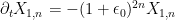
If we consider nonlinearities which are a finite linear combination of local cascade operators, then the equation (2) more or less collapses to a system of ODE in certain “wavelet coefficients” of . The precise ODE that shows up depends on what precise combination of local cascade operators one is using. Katz and Pavlovic essentially considered a single cascade operator together with its “adjoint” (needed to preserve the energy identity), and arrived (more or less) at the system of ODE

where ![{X_n: [0,T] \rightarrow {\bf R}}](https://s0.wp.com/latex.php?latex=%7BX_n%3A+%5B0%2CT%5D+%5Crightarrow+%7B%5Cbf+R%7D%7D&bg=ffffff&fg=000000&s=0&c=20201002) are scalar fields for each integer
are scalar fields for each integer  . (Actually, Katz-Pavlovic worked with a technical variant of this particular equation, but the differences are not so important for this current discussion.) Note that the quadratic terms on the RHS carry a higher exponent of than the dissipation term; this reflects the supercritical nature of this evolution (the energy
  is monotone decreasing in this flow, so the natural size of
  given the control on the energy is
  ). There is a slight technical issue with the dissipation if one wishes to embed (3) into an equation of the form (2), but it is minor and I will not discuss it further here.
In principle, if the mode has size comparable to  at some time
  , then energy should flow from to
  at a rate comparable to
  , so that by time
  or so, most of the energy of should have drained into the mode (with hardly any energy dissipated). Since the series
  is summable, this suggests finite time blowup for this ODE as the energy races ever more quickly to higher and higher modes. Such a scenario was indeed established by Katz and Pavlovic (and refined by Cheskidov) if the dissipation strength
  was weakened somewhat (the exponent
  has to be lowered to be less than
  ). As mentioned above, this is enough to give a version of Theorem 1 in five and higher dimensions.
On the other hand, it was shown a few years ago by Barbato, Morandin, and Romito that (3) in fact admits global smooth solutions (at least in the dyadic case  , and assuming non-negative initial data). Roughly speaking, the problem is that as energy is being transferred from to , energy is also simultaneously being transferred from to
  , and as such the solution races off to higher modes a bit too prematurely, without absorbing all of the energy from lower modes. This weakens the strength of the blowup to the point where the moderately strong dissipation in (3) is enough to kill the high frequency cascade before a true singularity occurs. Because of this, the original Katz-Pavlovic model cannot quite be used to establish Theorem 1 in three dimensions. (Actually, the original Katz-Pavlovic model had some additional dispersive features which allowed for another proof of global smooth solutions, which is an unpublished result of Nazarov.)
To get around this, I had to “engineer” an ODE system with similar features to (3) (namely, a quadratic nonlinearity, a monotone total energy, and the indicated exponents of  for both the dissipation term and the quadratic terms), but for which the cascade of energy from scale to scale
  was not interrupted by the cascade of energy from scale to scale
  . To do this, I needed to insert a delay in the cascade process (so that after energy was dumped into scale , it would take some time before the energy would start to transfer to scale ), but the process also needed to be abrupt (once the process of energy transfer started, it needed to conclude very quickly, before the delayed transfer for the next scale kicked in). It turned out that one could build a “quadratic circuit” out of some basic “quadratic gates” (analogous to how an electrical circuit could be built out of basic gates such as amplifiers or resistors) that achieved this task, leading to an ODE system essentially of the form


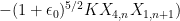
where  is a suitable large parameter and
  is a suitable small parameter (much smaller than
  ). To visualise the dynamics of such a system, I found it useful to describe this system graphically by a “circuit diagram” that is analogous (but not identical) to the circuit diagrams arising in electrical engineering:

The coupling constants here range widely from being very large to very small; in practice, this makes the  and
and  modes absorb very little energy, but exert a sizeable influence on the remaining modes. If a lot of energy is suddenly dumped into
  , what happens next is roughly as follows: for a moderate period of time, nothing much happens other than a trickle of energy into , which in turn causes a rapid exponential growth of (from a very low base). After this delay, suddenly crosses a certain threshold, at which point it causes and
  to exchange energy back and forth with extreme speed. The energy from then rapidly drains into
  , and the process begins again (with a slight loss in energy due to the dissipation). If one plots the total energy
  as a function of time, it looks schematically like this:

As in the previous heuristic discussion, the time between cascades from one frequency scale to the next decay exponentially, leading to blowup at some finite time  . (One could describe the dynamics here as being similar to the famous “lighting the beacons” scene in the Lord of the Rings movies, except that (a) as each beacon gets ignited, the previous one is extinguished, as per the energy identity; (b) the time between beacon lightings decrease exponentially; and (c) there is no soundtrack.)
There is a real (but remote) possibility that this sort of construction can be adapted to the true Navier-Stokes equations. The basic blowup mechanism in the averaged equation is that of a von Neumann machine, or more precisely a construct (built within the laws of the inviscid evolution  ) that, after some time delay, manages to suddenly create a replica of itself at a finer scale (and to largely erase its original instantiation in the process). In principle, such a von Neumann machine could also be built out of the laws of the inviscid form of the Navier-Stokes equations (i.e. the Euler equations). In physical terms, one would have to build the machine purely out of an ideal fluid (i.e. an inviscid incompressible fluid). If one could somehow create enough “logic gates” out of ideal fluid, one could presumably build a sort of “fluid computer”, at which point the task of building a von Neumann machine appears to reduce to a software engineering exercise rather than a PDE problem (providing that the gates are suitably stable with respect to perturbations, but (as with actual computers) this can presumably be done by converting the analog signals of fluid mechanics into a more error-resistant digital form). The key thing missing in this program (in both senses of the word) to establish blowup for Navier-Stokes is to construct the logic gates within the laws of ideal fluids. (Compare with the situation for cellular automata such as Conway’s “Game of Life“, in which Turing complete computers, universal constructors, and replicators have all been built within the laws of that game.)


197 comments
Comments feed for this article
14 January, 2015 at 9:49 pm
joe
Andreas, are you referring to me? or Prof. Tao
I have the complete equations but never submitted to any journals. Was hoping to help Prof Tao in submitting or co-author the papers since he has the deep mathematical skill and reputation on the subject.
15 January, 2015 at 12:35 am
Ainuru
See the research of 3D incompressible fluid, which is published at the end of 2014
http://www.smolensk.ru/user/sgma/MMORPH/N-43-html/cont.htm
The proximity of solutions of the Navier-Stokes and Euler equations given in a separate paragraph. The results are summarized for the Navier-Stokes equations in multidimensional space.
27 March, 2015 at 12:48 am
matthew miller
For Professor Tao,
If you’ll oblige me, what are the author’s views with regards overlap between a recent publication on FPU and your own on Naiver-Stokes?
Does this special business about 6 wave modes (and not another number) leading to dissipation in the absence of viscosity apply positively, negatively or neutrally to global regularity of the Naiver-Stokes problem – especially as regards your program/suggestion to establish finite time blowup?
.
27 March, 2015 at 1:01 am
matthew miller
From the above comment here’s the name of the paper, published in PNAS on the 23rd of March. Can also find on arXiv.
Route to thermalization in the α-Fermi-Pasta-Ulam system.
27 March, 2015 at 6:08 am
Terence Tao
As far as I can tell, the analysis in that paper is specific to the Fermi-Pasta-Ulam system and does not appear to have any analogue for Navier-Stokes evolution, which has quite a different dynamics.
27 March, 2015 at 2:12 am
shaurabh aggarwal
Can we solve navier stokes equation with more than 4 dimensions
1 January, 2022 at 8:19 am
Anonymous
yes. there have been papers in Journal of Fluid Mechanics dealing with 4th dimension turbulent channel flow.
28 March, 2015 at 12:00 am
Anonymous
It seems like the crux of the matter is to bound the ratio of the energy distributed in the high frequencies to the low frequencies, so extra dimensions should make the problem even harder.
28 March, 2015 at 12:24 am
Anonymous
I apologize if this is a wrong forum for these kind of queries, but there are hints that a global existence result of regular solutions would require a global _lower_ bound for the energy of the solutions. There are results such as Schönbek’s, which say that if the Fourier-transform of the solution does not vanish too fast at the origin, then the energy of the solution decays slower than C(1+t)^-(n/2+1). Is there a known lower bound for the energy for any initial data in, say, the Schwartz-class?
28 March, 2015 at 10:52 am
Terence Tao
I consider this unlikely: blowup or lack thereof is going to be decided by the dynamics of the high-frequency component of the solution, whereas questions of energy decay are mostly decided by the dynamics of the low-frequency components (as the result of Schonbek indicates). Note that if a solution has unusually rapid energy decay, then one should be able to modify that solution to one which does not exhibit such decay simply by placing an additional low-frequency component to the initial velocity that is supported sufficiently far away from the rest of the initial data that it does not significantly affect the dynamics of that data (other than by an approximately linear superposition of the original solution with the evolution of the low-frequency component). This suggests that the singularity behaviour of the solution is more or less decoupled from the energy decay behaviour. (Note also that the construction in my paper suggests that blowup can be achieved using arbitrarily small amounts of energy.)
29 March, 2015 at 8:32 am
Juha-Matti Perkkiö
Dear prof. Tao,
Of course the route from a lower bound of the energy to a possible long-time existence of regular solutions is far from obvious. However, they are at least somewhat connected already in a very primitive level: If there was a solution whose energy decays too rapidly, say at the exact rate E(t)=(T-t)^a for some interval [T’,T] and a<1, then the H^1-norm would blow up at t=T. This naive remark is of course not in discord with your argument, but it already suggests that energy decay and regularity are at least somewhat coupled.
30 May, 2015 at 2:16 pm
Andreas Z.
This is one of the most fascinating post I have read at your blog. If there any chance that you continue post about this topic and your progress or ideas? Thank you a lot! :)
2 June, 2015 at 10:59 pm
Sergey
Dear Dr. Tao, let me present my article regarding the general solution of Navier-Stokes Eqs.:
http://arxiv.org/abs/1502.01206
– I kindly ask you to give a few comments, if possible…
12 June, 2015 at 1:51 am
Daniel
Dear Prof. Tao,
It is kinda hard to imagine how it is possible to create blowups while obeying the energy identity. Is the key here “finite time”? If your fluid has to be ideal in this system and you are taking dissipation terms into consideration, doesn’t it mean that your fluid can be non-ideal, too? I mean, if your system actually needs dissipation to operate as gates, why can’t it work with non-ideal fluids that will come with intrinsic dissipation? It sounded to me like a system where the wires has to be perfect conductors but you put resistive components into the circuit so you can do the gating. Did I misunderstand what ideal fluid or dissipation is? Another question, is there a fundamental reason why this approach won’t work with electromagnetic waves?
-Kind regard, Daniel.
12 June, 2015 at 5:13 am
Terence Tao
The energy identity controls the total energy of the fluid, integrated over all of space, but it does not control the pointwise energy density of the fluid (or equivalently, the square of the speed of the fluid), because the energy could be concentrated in an arbitrary small ball of space. In particular, in the blowup scenario envisaged here, the energy remains bounded but is being concentrated into smaller and smaller balls, and in finite time one arrives at a singularity in which a finite nonzero amount of energy is supposed to concentrate into a single point, which cannot occur for a smooth solution to Navier-Stokes.
By “ideal fluid” here, I mean an incompressible fluid without dissipation, whereas Navier-Stokes models incompressible fluids with dissipation. So a system that is designed to work for ideal fluids does not work perfectly when one instead substitutes the viscous fluids modeled by Navier-Stokes. However, if one shrinks the system down to a very small spatial scale (and scales up the velocity field accordingly, keeping the total energy constant), this rescaling is effectively equivalent (in the sense of matching Reynolds number) to scaling down the viscosity to become very small while keeping the physical length scale unchanged, making the ideal fluid approximation much more accurate (and it will become exponentially more accurate if the system evolves as predicted to smaller and smaller scales). Because of this, I expect that if one can create the desired approximately self-similar dynamics for an ideal fluid (with suitable “error correction” coded in if necessary to give enough stability), then one can also obtain such dynamics for viscous fluids if one initialises the system to be supported in a sufficiently small scale (or equivalently, one assumes the viscosity parameter to be sufficiently small).
12 June, 2015 at 6:25 am
arch1
“…the energy remains bounded but is being concentrated into smaller and smaller balls, and in finite time one arrives at a singularity in which a finite nonzero amount of energy is supposed to concentrate into a single point…”
This reminds me of something I think I once read concerning the crack of a bullwhip (namely, that it results from the tip going supersonic).
1 July, 2015 at 9:56 am
rbcoulter
Hello Professor Tao: Is it necessarily so that the energy is finite at a point in the blowup scenario? Assuming that the energy density is infinite in the blowup scenario, I would imagine that one would need to take limits to calculate the actual energy at that point. For example, if r is the radius of a ball surrounding the blowup point, then the mass of the ball is proportional to r cubed. If the velocity blows up proportional to 1/r^n then the energy blows up 1/r^2n. Since the energy at the blowup point is the product of the energy density and the mass of the ball, only in the case of n = 1.5 will the energy be finite at the point. For n1.5 the energy at the point is infinite.
30 July, 2015 at 10:06 pm
danield
I wonder what could be shown if the fluid were acted on by an external force – say the fluid was a turbulent plasma under the influence of a magnetic field – and somehow altering that magnetic field to control the direction of the turbulence
basically using an external force to do this – ”the energy remains bounded but is being concentrated into smaller and smaller balls”
31 July, 2015 at 7:55 am
Terence Tao
It depends on how smooth the external force is, or equivalently how quickly it oscillates at small scales. If one applies a smooth external force, then by the time the energy is concentrated into a small ball, the force is effectively constant, and can be normalised to be negligible by applying a Galilean change of coordinates. (The analogy I sometimes use is that a smooth force is like the ability to manipulate an object with very fat, clumsy fingers; one do all sorts of macroscopic changes to the state with such a force, but it is difficult to obtain precise fine-scale control.)
If one allows for very rough external force, then one could certainly exhibit blowup as well – a singular external force can certainly produce a singular solution. But this is is rather easy to accomplish and doesn’t seem to shed much light on the global regularity question (which requires a smooth external force).
One possible interesting scenario, which has neither been constructed nor prohibited to my knowledge, is to find some singular (but still bounded velocity) initial data that leads to blowup (in the sense of, say, the L^3 norm of velocity diverging) in finite time, without the assistance of a singular external force. In principle, one could imagine singularities in the data being somehow sustained until the time comes that they are needed to guide the solution from one fine scale to an even finer scale. There is a little bit of hope that such a scenario could be constructed for active scalar equations such as SQG, where the scalar is transported and so “remembers” in some sense its initial configuration. This would still be fairly far from a finite time blowup from smooth data with smooth external force, though.
14 August, 2015 at 6:25 am
Anonymous
What do you mean by singular initial data (but finite velocity)? How can we generate a fluid motion with such data?
14 August, 2015 at 12:10 pm
Terence Tao
By “singular” I mean here “not smooth”, for instance the velocity may be bounded, while the derivative of the velocity (or related quantities such as the vorticity) are unbounded (or perhaps it is the second derivatives of the velocity are unbounded). This allows for nontrivial fine scale structure to the initial data which could conceivably be used to “steer” the solution through its evolution through finer and finer scales into finite time blowup.
25 August, 2015 at 1:26 am
Anonymous
There is a paper (arXiv:1104.3615 or CommMathPhys 312(3)) whose initial data is close to the type you mentioned. It was claimed that the critical case L3-velocity norm blows up in finite time from initial smooth data with compact support (i.e. finite initial energy in R^3). Apart from lack of convincing apriori bounds and a few technical glitches, one assumption made in that paper was velocity field (and pressure) might be split into two parts: one part is linear and governed by the Stokes system, and the rest by the NSEs. Moreover, the separation assumption was considered to hold independent of the size of the initial data, and of time interval ahead possible singularity. No justification and qualification were given. By the well-known NS regularity for small data, the assumption cannot be valid for arbitrary initial data. In general, the claimed out-of-bound condition (Theorem 1.1) at most implies that the assumed flowfield breaks down in finite time; the blowup does not necessarily represent a genuine singularity condition for the NSEqs. (Similar arguments apply to paper arXiv:1508.05313.)
12 June, 2015 at 6:01 am
Sergey_Ershkov
Dear Prof. Tao, as for ansatz in the reference arXiv.org above, the momentum equation of NSE has been presented as a system of PDE (each was solved accordingly): invariant for pressure, and the sum of 2 equations: – with zero curl for the field of flow velocity (viscous-free), and the proper Eq. with viscous effects but variable curl.
A solenoidal Eq. with viscous effects is represented by the proper Heat equation for each component of flow velocity with variable curl.
Non-viscous case is presented by the PDE-system of 3 linear differential equations (in regard to the time-parameter), depending on the components of solution of the above Heat Eq. The general solution of PDE-system above is composed of the solutions of 2 complex Riccati Eqs. (which are chosen to form such a composed solution as the real function in any case).
So, the existence of the general solution of Navier-Stokes equations is proved to be the question of existence of the proper solution for such a PDE-system of linear equations. Final solution is proved to be the sum of 2 components: – an irrotational (curl-free) one and a solenoidal (variable curl) components.
17 June, 2015 at 10:16 pm
Anonymous
Paper arXiv:1502.01206v3 is absolutely INCORRECT. Curl on every term in the large brackets in (2.1) equals to zero because curl(grad A)=0 for any scalar A. But the expression of 1st eqn in (2.3) does not vanish and is NOT the Bernoulli principle in general. Helmholtz’s decomposition of the velocity (vector) field has nothing to do with the (scalar) pressure. Eqns (2.3)-(2.5) are nonsense. It may be helpful to go back to basic textbooks.
18 June, 2015 at 12:17 am
Sergey_Ershkov
“Curl on every term in the large brackets in (2.1) equals to zero because curl(grad A)=0 for any scalar A.” – yes, this is true (this is trivial, obvious note). And what else?
“But the expression of 1st eqn in (2.3) does not vanish and is NOT the Bernoulli principle in general” – I don’t suggest it to be vanish or to be equal to Bernoulli invariant (I supposed it to be like ~ Bernoulli invariant).
I suggest to present 1 non-linear PDE (Navier-Stokes) as a sum of 3 parts: Bernoulli-like invariant, and 2 others (curl-free and with variable curl).
You should be more attentive when you read a text!
“Helmholtz’s decomposition of the velocity (vector) field has nothing to do with the (scalar) pressure” – I have no aim “to do with the (scalar) pressure”. I just present the vector gradient field of the scalar components of pressure is to be dependent on the appropriate components of the velocity field.
“Eqns (2.3)-(2.5) are nonsense” – this is my approach to represent of initial NSE as a sum of 3 Eqs. (I have explained it above already). Such decomposition is true, if we could find the proper solution to each of them.
“It may be helpful to go back to basic textbooks” – I kindly advise you not to be dubious and also you should be more attentive when you read any scientific material.
Kind regards!
18 July, 2015 at 7:51 pm
Anonymous
Ershkov’s solution is CORRECT and must enter in the basic textbooks as the most closer one to the problem.
4 August, 2015 at 4:54 am
Sergey_Ershkov
Thank you for your esteemed opinion, my unknown friend Anonymous (#2). We are under attack with you :) {I mean the enormous number of likes/dislikes}.
Yes, I think that my solution has been presented in a more general form than ever. But it concerns only the time-depending structure of solution; the space part is determined by 4 PDEs of 1-st order {for curl-free part of solution} – i.e., by 1 continuity equation and 3 “zero curl” conditions – and additionaly determined by the Heat-transfer Eq. {for the part of solution with variable curl}.
Such a decomposition – curl-free vs. variable curl – is defined by the fundamental Helmholtz theorem of vector calculus.
As for decomposition of one non-linear PDE (for curl-free part of solution) to the system of 1 invariant of Bernoulli-type + system of linear PDEs in regard to the time-parameter t: – of course, you should know a Caratheodory’s existence theorem – it proves the existense of a solution for such a case.
So, in a future it should be investigated properly the space part of a solution (I mean the solving of 4 PDEs of 1-st order above + Heat-transfer Eq.) as well as it should be calculated the appropriate estimations for energy of the flow – according to the demands of Clay Mathematics institute.
I hope that my first result (concerning the presentation of general solution of Navier-Stokes Eqs.) will make it possible to solve this problem by some unknown genius … if you have any questions regarding my paper or about some collaborations {may be, future mutual publications about NSE}, you could contact me through ResearchGate.
17 June, 2015 at 1:26 am
Sergey_Ershkov
Here below you will find the up-to-date reference, for your perusal:
“On Existence of General Solution of the Navier − Stokes Equations for 3D Non-Stationary Incompressible Flow”
http://www.dl.begellhouse.com/ru/journals/71cb29ca5b40f8f8,669062760250c799,0679e1964365ade8.html
18 July, 2015 at 8:23 pm
Anonymous
So many likes/dislikes
28 July, 2015 at 6:51 am
Lars Ericson
Regarding the self-replicating at finer scales von Neumann machine, would the ideas of digital physics be relevant? (https://en.wikipedia.org/wiki/Digital_physics) In digital physics, the universe is a cellular automata. There is nothing smaller than a single cell, and the speed of light is the “clock speed”, the rate at which information can move from one cell to the next. In that model, you can’t keep infinitely self-replicating at smaller scales, because you can’t replicate smaller than a single cell.
Also there is that intuition that computation = energy, in the sense that if I have an idle GPU it consumes 35W. When it is 100% utilized it consumes 235W and heats up. You can try to speed up the GPU by freezing it or by increasing the clock speed. At higher clock speeds, the GPU consumes quadratically more energy. The freezing also takes energy. Both of these imply a physical limit on miniaturizing computation. (http://electronics.stackexchange.com/questions/81344/is-cpu-gpgpu-heat-dissipation-quadratic-in-clock-frequency)
31 July, 2015 at 1:49 pm
Anonymous
NS regularity is a problem in pure mathematics, inspired by physics but not constrained by it. It’s set in a continuum so there is no “Planck constant”. It’s just like geometry was inspired by surveying but intuitions from surveying are of no use in understanding the Banach-Tarski paradox. You have to work out all the details, and in the case of NS, it’s hard enough that nobody has been able to do that.
3 August, 2015 at 6:01 am
Lars Ericson
It’s a thought experiment to make computers out of water that make tinier computers out of water. It’s a real experiment to take a chip and overclock it to make it go faster and then discover that you have to add a tower of liquid nitrogen so it doesn’t melt, and that the amount of energy consumption and concomitant required cooling grows exponentially (not quadratically as I said mistakenly in the post) with clock speed. Tiny fast computers need giant hot coolers so they can be tiny and fast. There are all kinds of physically-induced tradeoffs. These are experimentally observable. Theoretically, digital physics posits a lower bound (the cell) on even-tinier self-replication. John Wheeler posited the “it from bit” connection. (https://en.wikipedia.org/wiki/Digital_physics#Wheeler.27s_.22it_from_bit.22) Ed Fredkin posited that all things are discrete rather than continuous. (http://www.bottomlayer.com/bottom/finite-all.html) Cellular models explain the speed of light as the clock speed to move information from one cell to the next. (https://en.wikipedia.org/wiki/Speed_of_light_%28cellular_automaton%29)
A non-trivial thought experiment would take into consideration both the real, observable physical limits to computing, and the theoretical ones. So to say that NS is inspired by physics but not constrained by it is, pragmatically speaking, nonsense, because physically unconstrained solutions will have no physical relevance. Yes, you can mathematically construct an infinite sequence of numbers, but you can’t construct them all and pile them on a plate.
2 August, 2015 at 3:38 am
Anonymous
According to the official problem description (by the Clay Math. Institute), “… if there is a solution with a finite blowup time , then the velocity
  becomes unbounded near the blowup time.” (pages 2-3).
Therefore, it seems reasonable to expect that there is a (special) relativistic version of the NS equations without a finite blowup time.
2 August, 2015 at 7:11 pm
arithmetica
So who’s the dingus who downvoted all of Terry’s comments for no reason? What juvenile behavior.
3 August, 2015 at 12:14 am
Sergey_Ershkov
arithmetica, this is indeed juvenile behavior.
I suspect Anonymous as the main hooligan, who commented before you (see such an enormous number of likes/dislikes at his reply to me from 12-17 June 2015 as well as in my posts). This is unnormal behaviour.
As for me, I respect opinion of Dr.Tao.
21 August, 2015 at 10:39 am
Philip L
I saw your talk for the Einstein Memorial lecture, and it was interesting. Your method reminds me of several things, aside from of course cellular automata. Some automata are able to perform all computations, I suppose this includes non-linear dynamics.
1. Density functional theory. Density functional theory was originally used in chemistry to determine the spectrum of molecules. It allows approximation of a relatively intractable multi-body systems (i.e. electron-electron interaction, electron-nucleus interaction). It uses correlations (k-space mean field), providing additional structure (in the literal sense). The approximation can be refined by including 3-body correlations, 4-… etc. Ground states of main interest for chemists, physicists, and maybe molecular biologists because this is normally the only states that are thermodynamically accessible, and is the closest to the actual symmetry of the molecule. I also would like to mention the correspondence between (self interacting) solitons and the Schroedinger inverse problem.
2. Formation of (essential) singularities in finite time. This is also found in relativity, or calculations for formation of black holes. GR are nonlinear equations, which do not (yet?) have a proper Feynman diagrammatic perturbative description.
3. Diagrammatic expansion, This relates to points 1. and 2. . However, your work would differ in the sense that an exact description of non-renormalizable dynamics, where the approximation is refinable. The Feynman approximation involves linear interactions only (though QED might remain true for high amplitude/energy interactions, I think). There is no theory like this for gravity that I know. But my knowledge is humble.
Also, I learned in fluid mechanics Richardson-Kolmogorov cascade.
21 August, 2015 at 11:05 am
Philip L
There are also multi-time/scale approximations. There being the possibility of separable time scales, despite the absence of superposition. How do the frequencies of these modes change as parameters are changed? There may be a ‘topological phase transitions’ in the spectrum, and other global changes (e.g. bifurcations, cusps).
21 August, 2015 at 2:38 pm
Philip L
The GR case may be bit different. Here the singular is more like a 3 sphere in hyperbolic space. I have not encountered metrics with blackhole formation after a certain amount. It seems the topology or geometry is different in that case (maybe a 3 sphere cut out for example)? But there are theorems apparently about this.
17 September, 2015 at 5:19 am
Anonymous
It should be that it applies at ‘high energy’ instead of ‘large amplitude’, I believe.
1 October, 2015 at 3:42 pm
Sergey_Ershkov
Very interesting article of Michael Thambynayagam regarding the ansatz for resolving of Navier-Stokes eqs.:
http://arxiv.org/abs/1509.08766
– who is keen in the matter, should recognize this article to be worthy of a review at the Annals of Mathematics.
29 December, 2015 at 11:11 am
Gil Kalai
Let me try to give a more restrictive definition of what it would mean that
(*) “NS only supports ‘easy’ computation”.
This can have two purposes. The first, in case that Terry’s conjecture is correct and full computation is supported by 3D NS evolutions, (*) can be used to describe additional (implicit) conditions on realistic NS evolutions.
The second, more exciting, possibility is that (*) can actually be proved for 3D Navier-Stokes equation. This would be interesting on its own and may be a step for proving regularity.
In a comment above I proposed to take “easy computation” to be “bounded depth computation”. Namely (*) would mean that every computation described by NS can be approximated by bounded depth computation (circuit). A considerably weaker form of computation (and thus a much stronger form of (*)), would take “easy computation” to refer to the ability to describe (approximate) the computation by bounded-degree polynomials. (This is related to the notion of “noise-stability” used by Benjamini Schramm and myself.) A recent paper were “easy computation” of this kind was demonstrated to certain quantum systems is a paper by Guy Kindler and me
on Gaussian noise sensitivity and BosonSampling http://arxiv.org/abs/1409.3093
1 February, 2016 at 11:06 pm
Finite time blowup for an Euler-type equation in vorticity stream form | What's new
[…] been meaning to return to fluids for some time now, in order to build upon my construction two years ago of a solution to an averaged Navier-Stokes equation that exhibited finite time blowup. (I recently […]
9 February, 2016 at 10:47 pm
Anonymous
http://www.navier-stokes-equations.com/problem
This is an intersting website.
27 February, 2016 at 3:26 pm
rbcoulter
It seems that the averaged operator. T , can be viewed as the difference of the NS transport operator, TS, minus an external force (F).
Specifically T = NS – F
or F = NS – T
If F passes the conditions of (5) or (9) then this may acceptable as a blowup solution under the Clay rules.
The main question, in my mind at least, does F stay bounded at the blowup time?
In this interpretation the external force “pushes” or “is pushed” by the fluid. It can only be allowed to do this in a macro (smooth) way since any other way, that I can imagine, would violate conditions (5) or (9). The trick, however, is that at the instance of blowup, the last bit of energy must come naturally from the fluid itself to avoid the trivial blowup scenario of simply extracting energy at an infinite power density rate at the blowup point (from the external force field).
27 February, 2016 at 7:16 pm
Finite time blowup for a supercritical defocusing nonlinear wave system | What's new
[…] a question asked of me by Sergiu Klainerman recently, regarding whether there were any analogues of my blowup example for Navier-Stokes type equations in the setting of nonlinear wave […]
8 March, 2016 at 5:05 am
Finite time blowup for high dimensional nonlinear wave systems with bounded smooth nonlinearity | What's new
[…] sine-Gordon equation is not covered by our arguments. Nevertheless (as with previous finite-time blowup results discussed on this blog), one can view this result as a barrier to trying to prove regularity for […]
29 June, 2016 at 6:44 am
Finite time blowup for Lagrangian modifications of the three-dimensional Euler equation | What's new
[…] of the three-dimensional Euler equation“. This paper is loosely in the spirit of other recent papers of mine in which I explore how close one can get to supercritical PDE of physical […]
29 June, 2016 at 7:29 am
Jhon Manugal
Can you explain a little bit more about your “water computer” — I am afraid after reading this once or twice I could not find the operators.
I know that ODE can be discretized into recurrence relations (e.g. Euler Method), but that Euler Method “ought to” converge to the ODE.
Yet Cellular Automata can also be encoded as recurrence relations… therefore should be some vague relation between ODE and the model of computation of your choice.
All of that is excellent in theory except, in any one specific case I wouldn’t know how to build a computer. Not if my life depended on it.
29 June, 2016 at 8:14 am
Anonymous
Is there any explicit(!) lower bound (in terms of the initial data) for a possible blowup time?
30 June, 2016 at 11:56 am
Terence Tao
In two of the theorems, the data is carefully selected with an upper bound of the blowup time of 1, but the result does not say anything about generic data. For the first blowup result, which is more stable, if the initial data is supported in a narrow cylinder of width around the origin with a total circulation of
  , then the blowup time will be bounded by
  , which is consistent with dimensional analysis and also the Beale-Kato-Majda criterion (vorticity has units of inverse time, while circulation has units of length squared per unit time).
1 July, 2016 at 3:06 am
Anonymous
Is the implied constant in an absolute (i.e. independent of the initial data) and effectively computable?
Is there also a similar lower(!) bound for the blowup time?
1 July, 2016 at 7:43 am
Terence Tao
Assuming that the data is supported inside the cylinder of radius r (at least in a large neighbourhood of the origin), the constant is absolute. With enough control on higher derivatives of the initial vorticity, one should also be able to obtain a matching lower bound from the usual local existence theory (since one can morally rescale both time and space to normalise and
and  to both be comparable to 1), but I haven’t checked this.
16 August, 2016 at 2:39 am
Fahad
I know that the Navier-Stokes existence is really hard (probably that is the reason why you choose to solve variations of the Navier-Stokes) but I am just curious to know whether the energy dissipation can be used along with local existence and smoothness to prove global smoothness and existence in 2D or 3D? (like the one proposed by the Clay Mathematics Institute)
I am just a high school student, so, mostly my proof will be turned down by the math community.
19 August, 2016 at 10:30 am
Dejan Kovacevic
Fahrad- I hope that Terry will answer your question. However, regarding likelihood to be turned down by math community – don’t worry about that, follow your instincts, consult others, and make sure that you cover and analyze all possible issues and question all, even yourself. Keep questioning and finding the answers, as there is only one truth, regardless of communities of practice or interest. Eventually, what is truthful surfaces up as such, inevitably so.
20 August, 2016 at 3:43 pm
Terence Tao
This is discussed in detail in my other blog post https://terrytao.wordpress.com/2007/03/18/why-global-regularity-for-navier-stokes-is-hard/ . Basically, the answer is no, because the time of existence provided by the local theory can be arbitrarily small even when there is very little energy left to dissipate, and iteration of the local existence theory could thus conceivably lead to a convergent series which is consistent with finite time blowup. Note also that the equation considered in my paper here also has local existence and regularity as well as an energy dissipation inequality, yet still manages to exhibit solutions that blow up in finite time.
21 August, 2016 at 12:10 am
Fahad
Even I thought the same when I first encountered the problem initially. But, the energy dissipation in (28, Vorticity and Incompressible flow – Bertozzi, Majda) implies that before a singularity is formed, a small region of high energy is formed. This, in turn, forces the energy of the remaining regions
to be approximately close to zero. Let this region be Ω. the energy at the boundary ∂Ω is approximately zero compared to the absolute maximum in Ω. This almost forces the velocity field and its derivatives to be almost zero due to the above energy dissipation. Now, the proof proceeds as below link.
https://drive.google.com/file/d/0Bw5XWeTV9WGOLXhHMUxPUFFsY3M/view?usp=sharing
leading to the conclusion that the energy of the point where the energy is maximum in Ω, should decrease. Therefore, the solution remains in Schwartz space till infinity.
31 August, 2016 at 2:49 am
Fahad
Sir
I expect your view about my idea shown above :)
21 August, 2016 at 1:49 am
Tao Chi
hi… Terence Tao… my name is Tao Chi… and I Iive in Slovenia…
I saw… that you have deleted my video…
I give you a information… that I don’t care about this… that you have deleted… but I do care… that you didn’t give any reason for this action… or any explanation on my knowledge… which of course is not only mine… because it is a universal knowledge… like all of the knowledge… and that also means… that no human being should not give himself any special awards for any knowledge… everything what the human should do is… that he is a grateful for this knowledge… and that he apply this knowledge with ethics…
and ethics is… that you answer me on this message and that you explain me… what is wrong or what is right in my video…
if not… then I ask you… that you also delete my previously videos…
thank you…
P.S. If you see and work only with intelligence… you can be very wrong… because this is only a little part of wholeness…
intelligence is only a muscle which you can pumped up… but there are always a limits… like they are by muscles on the human body… but If you cross these limits… then you do more damage to yourself… than the benefits… by the intelligence we call this madness…
math… geometry… etc… are very welcome tools… for understanding how the universe work… but this tools are tools of the source… and that’s why we must use this tools with ethics… gratefulness… love… and in balance… if not… then you do more damage to yourself and to the others… than the benefits…
and that’s why the primes must be in interaction with non-primes… otherwise the intelligence will be in imbalance and in a state of ignorance…
with love and gratefulness…
TaoChi…
21 August, 2016 at 3:09 am
Fahad
Well, Terence Tao has put forth some requests (rules) of commenting in his blog, and it reads:
“I welcome comments from people with all kinds of mathematical backgrounds and levels of expertise; my only requests are that the discussions are kept constructive, polite, and at least tangentially relevant to the topic at hand. Comments which are spam, self-promoting, off-topic, or otherwise not fulfilling the above requests will be summarily deleted; repeated offenders in this regard may be subject to blocking. In particular, comments devoted primarily to promoting one’s own research are subject to deletion.”
And it probably is the reason why yours got deleted.
If you wish it to be promoted, formalise it in a form acceptable in the modern math community, and then publish it in a peer-reviewed journal. You can ask questions here, but it should be specific to the post (or thread).
21 August, 2016 at 4:48 am
Tao Chi
hi Fahad…
thank you for your explanation… I didn’t know for this rules… and certainly my presentation is not for promoting myself… it’s just the knowledge for which I am happy and I wish to shere… discuss and to use this knowledge with others…
with love and gratefulness…
TaoChi
25 August, 2016 at 4:44 am
Tao Chi
because I see… that you didn’t understand… what I have given to you… I will explain this with some other facts…
5 x 5 = 25
5 x 7 = 35
7 x 7 = 49
11 x 5 = 55
13 x 5 = 65
etc…
we see… that primes creates non-primes with a meaningful reason… because without them… they cannot work as wholeness or in harmony…
all systems like military systems… banking systems… etc… which for use only apply the prime numbers… are always in chaotic state… which proves everything what they do… and that’s why they must always fight for their own existence… because otherwise they will collapse immediately… and the reason for this is… because they don’t use the wholeness… and this is easy to see through perception where a man see only himself… and that’s why he is always in chaos… but when he see also a woman of course as equivalent… then suddenly everything is in balance… and this simple equation or algorithm… I have given to you in this video… etc…
all mathematicians… which will continuously search the meaning only in primes… they will always be in chaos… because they will not see the wholeness or harmony… and they will continuously chasing some ghost… which always disappears in the middle of some algorithm… what I have seen in my research… therefore… there are no twin primes… sexy primes… etc… because they are only here and there… and in mathematics and geometry… this is not a proof or algorithm… which work into infinity…
so… now is the decision… like always is… we can accept the solution or not… but the reality for this decision… always show us the real picture in our daily lives… what we see as…
action = reaction
cause = consequence
with love and gratefulness…
TaoChi…
25 August, 2016 at 5:57 am
Anonymous
???
25 August, 2016 at 6:32 am
Tao Chi
Anonymous… ask me… what you wish to know… and then I can give you an answer… if I can…
29 August, 2016 at 1:00 pm
Tao Chi
try to make a rectangle… hexagram… 8-gon… etc… only with primes… and you will see… that this is not possible… or you will see… that you get a chaos… and therefore non-primes are necessary and meaningful…
in real life… this is clearly to see… if we look for example through the monetary system… where is possible… that someone has a lot of money and someone has no money… with a simple math equation… we can clearly see… that there is no balance… therefore if we see only the primes as important… as if we see only the humans which are rich as important… then we get a chaos… because we cannot connect the lines… which can create a harmony… and this is shown in this video…
so… in this game the primes together with non-primes can make a harmony… balance… and of course a wholeness… but this is only math and geometry… in real life… we must use also other skills…
but in the monetary system we can create a balance… if we all have only one currency… and this can be simple created through the virtual world… like onecoin… bitcoin… etc… but by this currency… there are no more external owners… this means… that each individual… which will open this account and he will start to use this currency… it will become the sole owner of this account and all of the money on his own account… the beauty in this is… that all of this is similar… how the source of everything work… which is essentially 0… that means… that you start with 0… and then you have no limits… like the source don’t have no limits…
of course in this reality is only one law… and in this law is good to be honestly and sincerely… because this law is the source law… which cannot be changed… tricked or bypassed… and this law is…
action = reaction
or…
cause = consequence
this means… it is necessary… that we use the energy wisely… with ethic… gratefulness… in balance… and of course with love… like with the life energy… because only so… we can be in balance…
this is simple mathematical equation… which can create a beautiful life on this beautiful planet… and only we are capable to make this into the reality… thank you…
with love and gratefulness…
TaoChi…
31 August, 2016 at 2:46 am
Fahad
Hello Tao Chi
It is a humble request not to post irrelevant comments here. By this action most of the relevant ones are left behind not being able to get it replied. This post is about fluids, and yours is not at all related to this. Thus, It isn’t a good idea to post these kind of ideas here…
25 October, 2016 at 4:11 am
Viktor Ivanov
Dear Professor Tao,
Here are 3 counterexamples to your “supercriticality barrier”,: ‘The main purpose of’ the paper “Finite time blowup for an averaged three-dimensional Navier-Stokes equation“, submitted to J. Amer. Math. Soc.. 29 (3): 601–674.
1. Let us consider the 3D \int [(Z\cdot u)u](Z, r)A_r(Z)dZ = I, \int A_r(Z)dZ = 1, where A_r(Z) under r \rightarrow 0 is 3D Dirac delta function, u is a square integrable solution of the 3D Navier-Stokes equations. It is clear that I = 0, but almost all averages of (Z\cdot u)u yield I \neq 0. And \int _0^t I(r)/rdr , where t C > 0} z_ju_k^2(Z, r)e^{-|z_j|^2/r}dz_j/r^3dr \leq const., where u_k \neq 0 is a component of u and t < blowup time, and hence has no blowup time, but its averages can be \infinity.
3. I(r) = \int_0^\infty \int _0^\infty \int sign (z_j)e{-|z_j|h}|u(Z, r)|^2dZ\sum _{l \neq j} s_l^2 \prod_{l \neq j}ds_l , h = (\sum _{l \neq j} s_l^2)^{1/2}, I \leq \int_0^\infty \int _0^\infty e{-Ch} \sum _{l \neq j}s_l^2\prod_{l \neq j}ds_l | |u(., r)||^2 \leq C||u(., r)||^2, where C is a positive constant. So, \int_0^t I(r)dr \leq Ctsup_r ||u(., r)||, i.e., we have no blowup time. However, for almost any averages inside of the integrals, we have I(r) = \infty.
All 3 counterexamples-types are employed in my paper ‘A classical solution of the 3D Navier-Stokes and Euler problems’, which I sent you and asked to endorse for ArXiv, but have no response.
20 November, 2016 at 6:47 am
Viktor Ivanov
Here is the second counter example:
2. \int_0^t \int _{-\infty}^\infty z_ju_k^2(Z, r)e^{-|z_j|^2/r}dz_j/r^3dr \leq \int_0^t \int _{|z_j| > C > 0} z_ju_k^2(Z, r)e^{-|z_j|^2/r}dz_j/r^3dr \leq const., where u_k \neq 0 is a component of u and t < blowup time, and hence has no blowup time, but its averages can be \infinity
23 December, 2016 at 11:12 pm
Sketch of the Koch-Tataru theorem | Analysis and PDE Blog
[…] Mild solutions are constructed by considering the Navier-Stokes as a perturbation of the heat equation. In particular, the arguments used in the construction do not use the special cancellation structure (4) of the non-linearity. By themselves, they are not enough to solve the global regularity conjecture (see Tao’s discussion here). […]
29 December, 2016 at 6:59 am
Jon C
I must have read this article a long time ago, and have thought about this issue for a few years. My original motivation for thinking about ‘fluid machines’ was based from a science fiction novel called ‘Star Maker’ by Olaf Stapledon, which posits that the stars themselves can be alive. I wondered if perhaps they could indeed be alive. I also felt that water would likely possess this property of being able to ‘be alive’, but that probably the closest to being able to prove it would be to prove that it can sustain a self-replicating structure, and that structure can derive energy from an input to the entire system. I’m almost certain that the approach you describe here will one day be able to prove (or disprove) such an idea. Perhaps either vortices or solar granules (respectively) could function as a fundamental unit to perform these operations.
One key difference with Conway’s Game of Life (and most cellular automata, L-systems, etc), is that they do not concern itself with energy derivation from its environment – which I suspect is highly important. In other words – the behaviour of Navier-Stokes with a bounded input function might give just as interesting of a result as whether NS are regular or not without an input. To that end, I wonder if going on a tangent to investigate ‘simple fluid machines’ that could derive energy from simple fluid flows, and remain self-sufficient would be a worthwhile investment. This is similar to recent developments in astrobiology, which recognize that a fundamental characteristic of life is that it acts as a concentrator of negentropy: https://www.cambridge.org/core/journals/international-journal-of-astrobiology/article/div-classtitlethe-potential-for-detecting-life-as-we-donandapost-know-it-by-fractal-complexity-analysisdiv/81169D2F63946BCA4BB0DE6548597663
This approach, if able to reach a result, might be able to be mapped to the original problem (i.e. if a particular bounded input function that develops a ‘water machine’ can produce life / infinite blowup exists, can that be ‘mapped’ (folded up somehow) to a set of initial conditions without an input function that produce identical output for the original NS problem?)
31 March, 2017 at 5:45 am
itaibn
In section 6, I don’t see how you got inequality (6.71), which says that . Thinking about it heuristically I do not expect this inequality to be true: it should take
  time for the energy to be transferred for
  to
to  , which takes place before
  . During this time
  should grow to approximately
  , and exert an amplifying force of
  for time
  . Combined with the pumping from
  for time
  , the value of
  should be around
  , which is much greater than
  .
.
Skimming the rest of Section 6, I believe you infer this from inequality (6.108) of Proposition 6.12. In page 67 you justify Proposition 12 in terms of Proposition 6.13 and Proposition 6.15. However, the corresponding (6.117) of Proposition 6.13 gives a weaker inequality in terms of rather than
  .
.
I don’t expect any of this to effect the global structure of your proof, as you can just replace with
with  in (6.17), (6.32), (6.71), and (6.108).
[Thanks for this, this will be corrected in the next version of the ms. -T]
11 July, 2017 at 9:00 am
On the universality of potential well dynamics | What's new
[…] my previous work on blowup for Navier-Stokes like equations, I speculated that if one could somehow replicate a universal Turing machine within the Euler […]
25 July, 2017 at 7:39 pm
On the universality of the incompressible Euler equation on compact manifolds | What's new
[…] and curved manifold. This includes portions of the self-similar “machine” I used in a previous paper to establish finite time blowup for an averaged version of the Navier-Stokes (or Euler) equations. […]
21 August, 2017 at 8:06 pm
Sadik Shahidain
HI Terry,
Is there a relativistic form of the equations which has extra symmetry I could maybe try and use to our advantage?
Also lol at the analogy to turning this into a programming problem. I’m not really super good at math yet but programming I can get started on right aways! :)
Thanks,
Sadik
20 October, 2017 at 12:30 am
Anonymous
Is there any known result showing that the initial data needed for finite time blowup for the NS equations should be “very special” in some sense ?
It is very unlikely, but is there any known result showing the opposite (that is, such initial data is “generic”, or at least “not very special” in some sense) ?
20 October, 2017 at 10:52 am
Terence Tao
It is generally expected that finite time blowup should be avoided for “generic” initial data for 3D Navier-Stokes (for a suitable notion of “generic”), but there are not many rigorous results in this direction. One such is by Andrea Nahmod, Natasa Pavlovic, and Gigliola Staffilani, who show that almost all random data in a rough Sobolev space will at least admit weak global solutions to 3D Navier-Stokes, although their result does not establish regularity of these weak solutions (or even uniqueness of these solutions). But in general we have not been terribly successful in leveraging genericity hypotheses on initial data to obtain better existence and regularity results on the evolution than one could get from deterministically worst-case initial data of the same regularity class.
7 December, 2017 at 3:04 am
Anonymous
Is it possible that the solution to this problem depends on some still unknown invariant of the NS equations? Is there a known list (generated e.g. by Cartan’s method) of all such invariants ?
14 December, 2017 at 3:11 pm
Terence Tao
There have been efforts to systematically locate conservation laws for the Navier-Stokes and Euler equations, see e.g. https://mathscinet.ams.org/mathscinet-getitem?mr=3345572 . Thus far no usable new conserved or otherwise controlled integrals of motion have emerged. This is not to say that no such law will ever be found, but personally I would assume as a default hypothesis that this will not happen for Navier-Stokes (but for Euler there is a bit more chance, as this equation is more geometric and has more symmetries).
11 December, 2017 at 2:28 pm
Anonymous
It is very standard to applying the Leray projection {P} to divergence-free vector fields to eliminate the pressure term in the equation.The kinematic pressure p is determined uniquely by the velocity field up to an additive constant.
Is the other way around also correct: if p is know, can we expect that the velocity v can be recovered?
14 December, 2017 at 3:23 pm
Terence Tao
No, this should not be true: in three and higher dimensions, a scalar field such as does not have enough degrees of freedom to determine a vector field
  , even if one knows that vector field to be divergence free; one can perform Taylor expansions of
  and
and  around the origin and compare coefficients to see the underdetermined nature of
  from
from  more concretely. There is also the trivial redundancy that
  and
and  determine the same pressure
  .
.
14 December, 2017 at 4:47 pm
Anonymous
So the space dimension seems to be the main concern. What if one only works at the 2D NSE? (I’m very interested in the Taylor expansions idea but I don’t quite get it. Would you elaborate it a bit more?)
14 December, 2017 at 5:13 pm
Terence Tao
The Navier-Stokes equations are known to be globally well posed in two dimensions (where the equations are critical rather than subcritical), a result that I believe is due to Ladyshenskaya.
As for Taylor series: expand the pressure and the velocity components
  around the origin, assuming for sake of argument that all fields are analytic:
Taking divergences of the Navier-Stokes equation gives the equation relating the pressure to the velocity:
Equating coefficients up to order for some large
  , this gives a system
  (quadratic) equations involving the coefficients
  with
with  in terms of the specified pressure. The divergence-free condition
  yields a further
  equations. On the other hand, the number of coefficients
  with
with  is
is  . Thus there are significantly more unknowns than equations in the limit
  , and so this is a highly underdetermined system and one expects to find many velocity fields
  attached to each pressure
  .
.
15 December, 2017 at 5:11 am
Anonymous
Since one has the globally well posedness for the 2D NSE, can we expect then that the pressure can determine the velocity up to the redundancy (
 and
and  ) you mentioned? (It seems that one can pass the Taylor series check in the 2D case since

)
15 December, 2017 at 11:42 pm
Terence Tao
Writing in terms of a stream function
  as
as 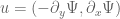 , it appears that the equation relating the pressure with the stream function is a Monge-Ampere equation
  . I’m not sure exactly what the uniqueness theory for this equation is; my understanding is that for the Dirichlet problem on a bounded Euclidean domain there is uniqueness due to a convex variational formulation, but on, say, the 2-torus, I am not familiar with the literature.
28 December, 2017 at 7:31 am
Pop Goes The Weasel: Navier Stokes and Compactness – bonefactory
[…] Tao’s fluid computer program for proving the impossibility of solving Navier stokes equations has not progressed, but it makes […]
13 March, 2018 at 5:29 am
Guy Cirier
Dear T. Tao,
Your blog is specialised on the Navier- Stokes equation (NSE):
∂
And I thank you very much. So, I propose a solution using your strategy 1, when the external forces don’t depend on the time. The demonstration is based on the following arguments:
At time , the velocity is a known smooth function of : . We deduce easily the pressure as the unique solution of the Poisson’s equation (under, for instance, Dirichlet’s conditions on the domain of ). Then, substituting and all the derivatives of by functions of in the NSE :
∂,
where is now a function of only. We observe:
. Then, we obtain an ordinary differential equation (ONSE) of in function of in a neighbourhood 𝒱of :
By this transformation, the unknown function is now and the solution is But, the conditions of existence of this solution are more easy to check. (For example, we see easily that the domain of , at the origin, must be inside the set if we want avoid turbulences).
Now, we can suppose at an arbitrary fixed time 0 that the velocity is known in function of the position : . We translate easily the demonstration from to and find the solution in a neighbourhood 𝒱of under new conditions of existence at . And so on.
We find other restrictive conditions of the existence of the solution of the ONSE. The solution exists under all these conditions.
Now, we observe that we can put in the function , any functions (smooth functions, derivatives, even unique solution of a functional or integro-differential equation of as the pressure of . The important condition is that will be smooth and not the linearity of the equations.
You may find more complete demonstrations in English in hal-01716814, v. 1 on the portal web of HAL : ( HAL https://hal.archives-ouvertes.fr ).
Could you say me what do you think about this paper?
If somebody is interested by my presentation, I am happy to receive all purposes or objections.
With my best regards.
Guy cirier
guy.cirier@gmail.com
28 March, 2018 at 8:58 am
Guy Cirier
Dear T. Tao,
It seems that you are interested by the Navier- Stokes equation (NSE):
∂
I think I have found a solution using your strategy 1, when the external forces don’t depend on the time.
The demonstration is based on the following arguments:
At time , the function of is a known smooth function: . We deduce easily the pressure as the unique solution of the Poisson’s equation (if, for instance, the domain of satisfies the Dirichlet’s conditions). Then, substituting (and all the derivatives of) by functions of in the NSE :
∂,
where is now a function of only. We observe:
. Then, we obtain an ordinary differential equation of in function of in a neighbourhood 𝒱of :
By this transformation, the unknown function is now and the solution is But, the conditions of existence of this solution are more easy to check. (For example, we see easily that the domain of must be inside the set if we want avoid turbulences at the origin).
Now, if we suppose at an arbitrary fixed time 0 that the velocity is known in function of the position : . We translate easily the demonstration from to and find the solution in a neighbourhood 𝒱of under new conditions of existence at . And so on.
We observe that we can put in the function , any functions (smooth functions, derivatives, even unique solution of a functional or integro-differential equation of as the pressure of . The important condition is that will be smooth and not the linearity of the equations.
You may find the demonstration in English in hal-01716814, v. 1 on the portal web of HAL : ( HAL https://hal.archives-ouvertes.fr ).
Could you say me what do you think about this paper?
With my best regards.
Guy cirier
guy.cirier@gmail.com
31 October, 2019 at 7:22 pm
Hobgoblins in Our Equations | Gödel's Lost Letter and P=NP
[…] Tao proved it can happen under a plausible modification of the Navier-Stokes equations of fluid dynamics. He […]
19 December, 2019 at 9:22 pm
Hussain
Dear Prof. Tao
I have a small question regarding your averaged equation, which might be trivial. Do you have a regularity criteria in terms of the Lipschitz constant of the solution? That is, say is the solution to your averaged equation, and suppose that
  and
and  . Can you control higher order norms of the solution on
  ?
?
This certainly is the case for the original Navier-Stokes system, due to, e.g., Beal-Kato-Majda criteria. One can also rather simply prove this by direct energy estimates. You do mention in your paper that bounds on the original bilinear operator may not carry over to the averaged one, and I was wondering if this is one such bound.
Many thanks in advance,
Hussain
20 December, 2019 at 9:21 am
Terence Tao
I believe for the specific bilinear operator I use for the blowup example there is a suitable endpoint paraproduct estimate which allows one to obtain this sort of regularity result, though for the general averaged bilinear operators in the class I describe in the paper there may not be such an estimate. On the other hand, I do not know if one can extend the Beal-Kato-Majda criterion (assuming only control of the vorticity) to my equation because it does not have a usable vorticity equation.
31 January, 2021 at 7:16 am
Navier
What is a logic gates that respects ideal fluid? You only need one of the universal gates.
14 May, 2021 at 12:20 am
To cheer you up in difficult times 23: the original hand-written slides of Terry Tao’s 2015 Einstein Lecture in Jerusalem | Combinatorics and more
[…] topic of Tao’s lecture was discussed on Terry’s blog (also here and several other posts), here on my blog, on SO, on GLL, on Quanta Magazine, and in […]
25 December, 2021 at 9:00 pm
Dwight Walsh
As I noted in Dr. Tao’s previous posting at https://terrytao.wordpress.com/2007/03/18/why-global-regularity-for-navier-stokes-is-hard/, he makes the assertion “…, but we will not need to study the pressure here” without references or supporting arguments. The grad p term, however, cannot be negligible compared to the nonlinear transport term since the sum of these two terms must have a zero divergence. In fact, the very purpose of the grad p term is to maintain a zero divergence of the right-hand side of the NS equation. Then, in the analysis that follows, he discusses the possibility of a blowup occurring as a result of energy being shifted to successively smaller space scales due to only the non-linearity of the transport term. Therefore, I believe the results of both this article and the earlier posting are invalid.
In the paper I posted at http://www.navierstokessmoothsolutions.com, however, I show that when grad p is correctly taken into account, then no such blowup is possible.
25 December, 2021 at 9:19 pm
Daniel
You are way off here Dwight. Prof Tao never said grad p is negligible.
25 December, 2021 at 11:59 pm
Dwight Walsh
Then what is Prof. Tao assuming about p and grad p? After his statement about not needing to study the pressure here, he never once mentions it. He merely argues intuitively that the viscosity and transport terms are “fighting” with each other over dominance of the solutions.
Then he makes “scaling” arguments to claim that a blowup could occur as a result of energy being shifted into progressively smaller scale sizes. In summary, Dr. Tao’s methods and arguments here are far from complete and no one knows how he is maintaining a zero divergence of the fluid velocity.
In my solution, however, I keep the NS equation intact by not using “scaling” or “averaging” methods, and I show existence and smoothness of solutions to this equations.
28 December, 2021 at 11:30 am
Dwight Walsh
All right, you thumb-downers — No one is stopping you from shooting down my arguments. So please do so! Otherwise, you will only convince me more and more that you have no ground to stand on.
25 December, 2021 at 11:09 pm
Anonymous
It is quite comical that you think you solved the millennium problem but are apparently unaware of the Leray projection.
26 December, 2021 at 12:14 am
Dwight Walsh
Wrong! I am well aware of the Leray projection. I am also aware, however, that it is not needed for solving the NS Millennium Problem and may actually complicate matters.