Polymath8b, VIII: Time to start writing up the results?

9 February, 2014 in math.NT, polymath | Tags: polymath8 | by Terence Tao

This is the eighth thread for the Polymath8b project to obtain new bounds for the quantity

$\displaystyle H_m := \liminf_{n \rightarrow\infty} (p_{n+m} - p_n),$

either for small values of ${m}$ (in particular ${m=1,2}$ ) or asymptotically as ${m \rightarrow \infty}$ . The previous thread may be found here. The currently best known bounds on ${H_m}$ can be found at the wiki page.

The big news since the last thread is that we have managed to obtain the (sieve-theoretically) optimal bound of ${H_1 \leq 6}$ assuming the generalised Elliott-Halberstam conjecture (GEH), which pretty much closes off that part of the story. Unconditionally, our bound on ${H_1}$ is still ${H_1 \leq 270}$ . This bound was obtained using the “vanilla” Maynard sieve, in which the cutoff ${F}$ was supported in the original simplex ${\{ t_1+\dots+t_k \leq 1\}}$ , and only Bombieri-Vinogradov was used. In principle, we can enlarge the sieve support a little bit further now; for instance, we can enlarge to ${\{ t_1+\dots+t_k \leq \frac{k}{k-1} \}}$ , but then have to shrink the J integrals to ${\{t_1+\dots+t_{k-1} \leq 1-\epsilon\}}$ , provided that the marginals vanish for ${\{ t_1+\dots+t_{k-1} \geq 1+\epsilon \}}$ . However, we do not yet know how to numerically work with these expanded problems.

Given the substantial progress made so far, it looks like we are close to the point where we should declare victory and write up the results (though we should take one last look to see if there is any room to improve the ${H_1 \leq 270}$ bounds). There is actually a fair bit to write up:

Improvements to the Maynard sieve (pushing beyond the simplex, the epsilon trick, and pushing beyond the cube);
Asymptotic bounds for ${M_k}$ and hence ${H_m}$ ;
Explicit bounds for ${H_m, m \geq 2}$ (using the Polymath8a results)
${H_1 \leq 270}$ ;
${H_1 \leq 6}$ on GEH (and parity obstructions to any further improvement).

I will try to create a skeleton outline of such a paper in the Polymath8 Dropbox folder soon. It shouldn’t be nearly as big as the Polymath8a paper, but it will still be quite sizeable.

135 comments

Comments feed for this article

10 February, 2014 at 5:02 am

tou

nice result!

10 February, 2014 at 7:31 am

GilYoung Cheong

I like this result because it shows me how important it is to understand other mathematicians’ ideas (and collaborate).

10 February, 2014 at 7:51 am

Terence Tao

A correction: when trying to use our various tricks to improve the $H_1$ bound on Bombieri-Vinogradov, the support of F can range in the quite large simplex $\{ t_1+\dots+t_k \leq \frac{2k}{k-1}\}$ , not just $\{t_1+\dots+t_k \leq \frac{k}{k-1} \}$ . So the epsilon in the “epsilon trick” can go all the way to 1 without difficulty, which could lead to a sizeable improvement by passing from $M_k$ to $M_{k,\varepsilon}$ (without even touching the region outside the simplex $\{ t_1+\dots+t_k \leq 1+\varepsilon\}$ . This might be computable using some variant of the numerics used for the $M_k$ problem, since we are still only integrating on simplices and not imposing any moment conditions.

10 February, 2014 at 9:05 am

Aubrey de Grey

Let’s hope so! Pace mentioned in https://terrytao.wordpress.com/2014/01/08/polymath8b-v-stretching-the-sieve-support-further/#comment-262427 that there are issues with multiplying and integrating polynomials of the form $(f(2-e_1)^k e_k)_{1,\ldots, k}$ – I don’t know whether that’s the main issue here. If it is, maybe it will be mitigated by optimising F first and then epsilon rather than the other way around (see https://terrytao.wordpress.com/2014/01/08/polymath8b-v-stretching-the-sieve-support-further/#comment-263500 ) and/or by restricting F to monomials with fewer than k variables. On the latter issue, I tried (I think correctly) modifying Pace’s code for k=3 to explore F’s whose monomials were restricted to just one variable (so in the d=2 case eliminating the xy, xz and yz terms) and the loss in M was very small (it still topped 1.99), so I suspect there is value there, even if there is no Lagrange-based argument that the optimal F will still be found.

11 February, 2014 at 11:03 am

Eytan Paldi

But (if I understand correctly) this means that for $\theta = 1/2$ we may take $R = \frac {2k}{k-1} \mathcal R_k$ which seems “too good to be true” (since then 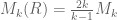$M_k(R) =\frac {2k}{k-1} M_k$ which for $k=2$ gives $M_2(R) = 4 M_2 > 4$ – implying unconditionally the twin prime conjecture!) Therefore, some clarification is needed.

11 February, 2014 at 11:33 am

Terence Tao

Well, one still has the vanishing moment conditions to deal with; F can range in $\frac{2k}{k-1} {\cal R}_k$ , but its marginals must stay supported in $(1+\varepsilon) {\cal R}_{k-1}$ if we wish to use the $J_{\varepsilon}$ functional (i.e. integration on $(1-\varepsilon) {\cal R}_{k-1}$ .

11 February, 2014 at 11:51 am

Eytan Paldi

Do you mean that the new relaxation is only for the support of $F$ but not for the supports of the marginals?

11 February, 2014 at 12:20 pm

Terence Tao

Yes… although on rechecking what I said, I realise now that I screwed up a little, and need to correct my correction: using only Bombieri-Vinogradov, one can enlarge the support of F to be as large as $2 {\cal R}_k$ (basically using the trivial distribution properties of the constant function 1), but not $2 \frac{k}{k-1} {\cal R}_k$ (this requires GEH, which we no longer have). Sorry about that. (One more reason to start writing up the results is so that these things can be clarified properly…)

11 February, 2014 at 12:36 pm

Aubrey de Grey

Terry, could you please elaborate on this? – I thought that the equivalent of GEH was indeed known for theta=1/2, courtesy of Motohashi?

11 February, 2014 at 2:38 pm

Terence Tao

I meant that to get up to $2\frac{k}{k-1} {\cal R}_k$ at the $\theta=1/2$ level requires GEH for $\theta=1$ , which is still a conjecture. From GEH for $\theta=1/2$ , which was indeed proven by Motohashi, one can get the support up to $\frac{k}{k-1} {\cal R}_k$ , but this is superseded by the support of $\frac{1}{\theta} {\cal R}_k = 2 {\cal R}_k$ that one can get just from the trivial distributional properties of the constant function 1.

10 February, 2014 at 8:02 am

Terence Tao

Just to repeat something from the previous thread: it looks like two of the eight vanishing marginal conditions $M_1=\dots=M_8=0$ are actually unnecessary in the $\varepsilon=1/4$ case, which could lead to either an improvement of the bound, or the ability to clean up the optimiser, e.g. by lowering the degree or by approximating the nasty fractions by cleaner fractions. Specifically, we need to test the marginals in the trapezoidal region $\{ x \geq y \geq 0; 5/4 \leq x+y \leq 3/2\}$ .

The M7=0 condition takes care of the triangle where $x \leq 3/4$ .

The M5=0 conditiont akes care of the large trapezoidal region where $x \geq 3/4$ and $y \geq 1/4$ .

What’s left is the parallelogram $\{ 0 \leq y \leq 1/4; 5/4 \leq x+y \leq 3/2\}$ . One can divide this parallelogram into four triangles, depending on whether $x$ is larger than 5/4 or not, and whether $x+2y$ is larger than 3/2 or not.

The conditions M1=0, M2=0, M3=0, M4=0 then handle the triangles $\{ x+2y \geq 3/2, x \geq 5/4\}$ , $\{ x+2y \leq 3/2, x \geq 5/4\}$ . $\{ x+2y \leq 3/2, x \leq 5/4\}$ . $\{ x+2y \geq 3/2, x \leq 5/4\}$ respectively.

The conditions $M6=0, M8=0$ do not appear to be needed in the $\varepsilon=1/4$ case, although they do show up for larger values of epsilon.

Another minor simplification: the first integral in the expression for I6 is trivial in the $\varepsilon=1/4$ case, although this only leads to a slightly simpler exposition rather than any numerical gain.

10 February, 2014 at 8:43 am

Aubrey de Grey

If Pace can make what is presumably an easy change to his code (I tried to work out for myself what change is needed, but I’m still too new to Mathematica), I’d be happy to play with it and seek such improvements. (Pace told me that he is busy with other projects at present and lacks the time to do much more on this.)

10 February, 2014 at 9:05 am

Pace Nielsen

Indeed I am! (But it was a simple change, as you said. Just had to change the type of rational approximation and drop the two marginal conditions.)

10 February, 2014 at 9:10 am

Aubrey de Grey

Many thanks Pace. If you email me the new notebook I’ll probably tinker with it to see if smaller degrees can now be used.

10 February, 2014 at 9:03 am

Pace Nielsen

Dropping the M6 and M8 conditions, and approximating the entries of the resulting optimized vector to within a thousandth, the following somewhat simpler fractions should still suffice:

FA= 1 – (1291 x)/1000 + (104 x^2)/125 – (659 y)/500 + (111 x y)/125 + (
1099 y^2)/1000 – (1257 z)/1000 + (637 x z)/1000 + (56 y z)/125 + (
839 z^2)/1000

FB= 57/100 – (303 x)/500 + (117 x^2)/250 – (136 y)/125 + (227 x y)/500 + (
133 y^2)/125 – (303 z)/1000 – (9 x z)/125 + (57 y z)/250 + (
37 z^2)/250

FC= 17/50 – (657 x)/1000 + (227 x^2)/500 – (13 y)/20 + (581 x y)/1000 + (
21 y^2)/40 – (9 z)/1000 + (3 x z)/1000 + (3 y z)/200 + z^2/250

FD= 0

FE= 4711/16000 – (199 x)/2000 – (29 x^2)/1000 – (2101 y)/2000 + (
413 x y)/1500 + (33 y^2)/25 – (19 z)/125 – (13 x z)/1000 + (
31 y z)/125 + (7 z^2)/600

FS= 2409/16000 – (9 x)/80 – (61 x^2)/1000 – (493 y)/1000 + (
401 x y)/1500 + (73 y^2)/125 – (73 z)/500 + (59 x z)/1000 – (
9 y z)/250 + (79 z^2)/1000

FT= -(471/8000) + (367 x)/4000 – (7 x^2)/200 – (1133 y)/2000 + (
9 x y)/25 + (129 y^2)/200 + (373 z)/1000 – (103 x z)/400 – (
3 y z)/200 – (89 z^2)/400

FU= -(2548925261/40960000) + (378889 x)/500 – (1486281 x^2)/500 + (
2109761 x^3)/500 – (1806913 x^4)/1000 – (823 y)/1000 + (
1028 x y)/125 – (1276175057 x^2 y)/20800000 + (5231 x^3 y)/40 – (
604 y^2)/125 + (465755881 x y^2)/10400000 – (
33092919 x^2 y^2)/400000 + (1941 y^3)/500 – (21127 x y^3)/1000 + (
28 y^4)/125 + (705 z)/8 – (196213 x z)/200 + (
130643581043 x^2 z)/41600000 – (1270877 x^3 z)/500 + (
51 y^2 z)/16000 – (91952143 z^2)/3328000 + (
619313327 x z^2)/2080000 – (18524 x^2 z^2)/25 + (3 y^2 z^2)/5000 – (
2561 z^3)/1000 + (4869 x z^3)/500 – (9 z^4)/200

FG= -(2695785741/10240000) + (2173499391 x)/1280000 – (
12242903151 x^2)/2560000 + (52219413 x^3)/10000 – (
1806913 x^4)/1000 + (96070478631 y)/83200000 + (
1007933539 x y)/20800000 + (179877147 x^2 y)/2600000 – (
36827397 x^3 y)/25000 – (669613358991 y^2)/166400000 – (
1310180447 x y^2)/2600000 + (10110876 x^2 y^2)/3125 + (
19620542273 y^3)/3900000 – (17662711 x y^3)/12500 – (
1806913 y^4)/1000 + (104838525951 z)/166400000 – (
126851653541 x z)/41600000 + (15524384001 x^2 z)/2600000 – (
20898059 x^3 z)/6250 – (1531159429 y z)/640000 + (
14385788557 y^2 z)/2600000 – (20898059 y^3 z)/6250 – (
91851736253 z^2)/166400000 + (4642413047 x z^2)/2600000 – (
738812349 x^2 z^2)/400000 + (2655529 y z^2)/1625 – (
756836049 y^2 z^2)/400000 + (1081347403 z^3)/5200000 – (
33823447 x z^3)/100000 – (36827397 y z^3)/100000 – (
2238403 z^4)/80000

FH= -(37/250) + (71 x)/500 – (109 x^2)/1000 + (6 z)/125 – (3 x z)/1000 – (
9 z^2)/250

The complicated forms for the F_G and F_U pieces arise when guaranteeing the other marginal conditions still hold.

(By the way, I concur that that when epsilon=1/4, the M6 and M8 conditions are indeed irrelevant. Sorry for not putting more description into the files I created earlier about when the different vanishing marginal conditions arise.)

10 February, 2014 at 9:26 am

Eytan Paldi

Is it possible to simplify further these expressions by dropping the vanishing constraint on $FD$ ?

10 February, 2014 at 2:46 pm

Pace Nielsen

There is no constraint forcing the D-component 0. It just happens that this is the optimal choice. (The D-region only contributes to the I-integral, and doesn’t appear in any of the J-integrals, so anything nonzero only hurts us.)

11 February, 2014 at 11:15 am

Terence Tao

This checks out (I = 0.03057904694, J = 0.06116827145, all marginals other than M6 and M8 OK). [I had initially gotten ridiculous answers, but on inspecting which marginal conditions had failed, I realised I had input in the FU data incorrectly.] I’ll update the wiki with this simplified example.

Nice to see that we’ve flipped from playing “Zeno’s paradox” to playing “Jenga”: what is the minimally complex construction we can do to stay above 2?

11 February, 2014 at 4:57 pm

Aubrey de Grey

Thanks for these values Terry – their ratio is 2.0003, as against the previous 2.00003 with that degree set – maybe there’s more simplification to be had here. I also notice the curiosity that FU and FH have some monomials missing (FU lacks yz, (y^3)z, y(z^2) and y(z^3) and FH lacks y, y^2, xy and yz) – is that to be expected from the elimination of those marginals?

11 February, 2014 at 5:13 pm

Eytan Paldi

It is possible that the vanishing of the additional coefficients is due to the approximation (within 0.001) that Pace made (further simplification is possible by slightly increasing the 0.001 value – but of course not too much).

11 February, 2014 at 5:30 pm

Aubrey de Grey

I had considered that, but I’m dissuaded from it by the fact that the coefficients of those monomials of FH in Pace’s original post (where they were given in floating-point) were actually the largest of all the FH monomials.

However, a further look back at that post reveals that FU (and only FU) is missing six monomials – yz, (y^2)z, (y^3)z, y(z^2), (y^2)(z^2) and y(z^3). The two that are missing there but not in the more recent FU (namely (y^2)z and (y^2)(z^2)) have the smallest values of all F monomials, so your suggestion is more likely for FU. And even though some of the other polynomials are very similar in all coefficients in the two cases, others are very different, so there’s probably nothing in this.

11 February, 2014 at 5:45 pm

Eytan Paldi

From the denominators of the coefficients it seems that their approximations (within 0.001) are decimal fractions (probably with denominator 1000), therefore further simplification is possible by such approximations (within the same tolerance) – using fractions (not necessarily decimal) having minimal denominators.

11 February, 2014 at 6:01 pm

Eytan Paldi

The numerical coefficients of the polynomials in the recent post are not necessarily close to the corresponding ones in the former post since the optimization in the recent post is different (without two marginal constraints M6 and M8).

11 February, 2014 at 6:43 pm

Aubrey de Grey

Eytan: yes, I agree. Regarding further simplifications, I think it could also be interesting to see whether the elimination of M6 and M8 causes M to rise enough, when leaving the precision as before, to allow the various degrees to be lowered further – or, conversely, whether with modestly increased degrees (and maybe with the monomials featuring all three variables added back in) the denominators can be made really small. It will then, of course, be a matter of taste which such variant is viewed as the simplest.

12 February, 2014 at 4:17 am

Eytan Paldi

Perhaps the last simplification should be to make (by multiplying with the common denominator) all the coefficients integers (hopefully not “too big”).

10 February, 2014 at 8:07 am

Anonymous

“ $M6 = 0, M8 = 0$ ” –> “ $M_6 = 0, M_8 = 0$ ”

Just to make it more readable, should all of the math expressions be typeset using LaTeX?

[The notation is from these notes http://www.math.byu.edu/~pace/BddGapsSize6.pdf, with the variable names being formatted for Mathematica rather than for LaTeX use. -T]

10 February, 2014 at 11:09 am

James Maynard

I’ve been away for the past week, but I’ve just gone through Pace’s decompositions for the $H_1\le 6$ result.

I was a bit concerned about the possibility of making a careless error in all the decompositions or when typing it into the computer, so I wrote some code to automatically do the I and J integral decompositions. This naturally splits the integrals up into many more parts and so the code takes a lot longer to run, but I’m happy to confirm that I get exactly the same quadratic forms and the same bound of $2.0009$ when using the same polynomial decomposition and same marginal conditions as Pace used.

I noticed that for $\epsilon=1/4$ the $M6$ and $M8$ conditions are not necessary, and I also noticed that one gets a small numerical improvement to about 2.012 if one doesn’t restrict to polynomials with monomials involving two of the variables.

I think that since the automatic decompositions give exactly the same result, this is fairly strong evidence that all of Pace’s decompositions are correct and the $H_1\le 6$ result holds.

10 February, 2014 at 11:18 am

Aubrey de Grey

2.012 is quite a big improvement! I imagine the improvement will be less for the version that’s just been Maple-validated, though, since in that case (because most of the degrees are lower) the total number of monomials will only rise from 132 to 140.

10 February, 2014 at 11:28 am

Terence Tao

This is great news! So the $H_1 \leq 6$ result is now confirmed twice, and we also have a significantly larger margin of safety in case there is still something we all missed. Well done to everyone involved :)

Amusingly, this means that both of the Polymath8b results on $H_1$ will improve upon the corresponding results in your paper by a factor of two.

10 February, 2014 at 11:46 am

James Maynard

Ooops, I meant $2.0012$ , not $2.012$ – not such a huge improvement.

10 February, 2014 at 4:46 pm

Pace Nielsen

James, did you try to do the computation without splitting the F-region into the S,T,U pieces? I have a suspicion that it may be possible to still get $M\geq 2$ (especially without the two unnecessary marginal constraints).

11 February, 2014 at 8:13 am

James Maynard

Pace: Using degrees 5 and 2 as before, and keeping the F region in one piece (and without using the M6 and M8 marginal conditions) I get a lower bound of 2.000146 – just over the line.

11 February, 2014 at 8:39 am

Aubrey de Grey

James: one other setting that I don’t think has been explored yet is the extended prism with z ranging up to 2 rather than only 1 (per your Jan 27th observation about using GEH maximally). Since that prism has volume 1 as against only 9/16 for the untruncated simplex, there seems to be a pretty good chance that it would give better numerics and thus permit a cleaner F (with lower degrees and/or simpler fractions). Can your older code exploring the prism be easily adapted to this new setting?

11 February, 2014 at 9:08 am

Aubrey de Grey

Apropos: might there also be the possibility that a carefully-chosen, superficially sub-optimal epsilon would improve the prism’s numerics by obviating some of the vanishing marginal constraints, as we just saw with the simplex for epsilon=1/4? Recalling that the prism’s partial non-symmetry might motivate the use of two different epsilons, this might be a rather complex issue to explore…

11 February, 2014 at 12:07 pm

James Maynard

Aubrey: It should be easy enough to do this – it just requires me to choose on which regions we have our function being polynomial, to input the marginal conditions and to make a couple of adjustments for the fact it is no longer symmetric. I’ll try to put something fairly simple together and see what comes out. That said, I’m away in Illinois as of tomorrow, so I’ll probably only be able to report back next week

17 February, 2014 at 11:35 am

James Maynard

Aubrey: I made the modifications to look at the prism. Splitting the polytope up according to the ordering of x+z,y+z,1-e and 1+e gives a decomposition into 12 regions, and using degree 5 approximations I get a lower bound of about $1.965..$ (ignoring the trivial constructions which give a bound of exactly 2). It seems that one can increase this bound quite a bit (this seems a way from having converged), but it looks like unfortunately the prism isn’t going to give a simpler answer than we have already since we’d need more decompositions or higher degrees.

17 February, 2014 at 11:56 am

Aubrey de Grey

Interesting! Many thanks for this James. I wonder whether anyone has any intuition as to why there isn’t a reasonably tight correlation between polytope volume and M when other aspects are kept equal? I mean, the correlation should not be perfect, because different partitionings give different marginal constraints of different effective severity, but still it seems odd that the elongated prism’s being nearly twice as large as the untruncated simplex is outweighed by other factors.

11 February, 2014 at 8:59 am

Pace Nielsen

Thanks! That should simplify the exposition when we write this up.

12 February, 2014 at 5:53 pm

Aubrey de Grey

As one additional data point, in this configuration it’s possible to reduce all degrees except F and G to 2 and keep just above 2 (2.000066 to be precise), but only by including monomials with all three variables.

10 February, 2014 at 11:44 am

James Maynard

I think it should be numerically feasible to incorporate the epsilon trick into the existing numerical routine with only a slight slowdown.

The key observation for the numerical calculations to work was that it is easy to analytically calculate the $k$ -dimensional integrals of monomials
$\prod_i t_i^{a_i}$
over the simplex $\sum_i t_i<1$ , which allows us to easily calculate the I integrals. For the J-integrals we only need to perform a one-dimensional integral and then an integral of the above type (and provided the degree is suitably small, we can binomially expand to write the J integral of a monomial in terms of monomials as above, so everything remains feasible).

The same observation holds true with the epsilon-trick: we can still analytically write down the integral of a monomial over the simplex $\sum t_i<1+e$ or $\sum t_i<1-e$ . We can still use the binomial expansion to do the first one-dimensional integral for the J-integrals when the degree is reasonably small.

The only thing that we've lost when using the $\epsilon$ trick is that we were also using the fact that we also had a simple basis when we considered
$(1-\sum t_i)^a\prod_i t_i^{a_i}$ ,
and this allowed us to roughly double the degree of polynomial used. We can re-write our integrals in a similar form, but it would require another binomial expansion, and I don't know how costly (timewise) that would be. I think that overall this shouldn't pose too much of a problem, however, and so I think the $\epsilon$ trick should be OK to use. I don't have a good intuition of how much gain we should expect from it, though.

10 February, 2014 at 12:13 pm

Aubrey de Grey

I’m unclear as to how the epsilon trick is dovetailing with other available tricks. The availability of the simplex of size 2, though not 2k/(k-1), originally arose as part of the discussion of expanding R’ to R’’. Is the current line of thinking that a large epsilon basically substitutes for that expansion to R’’ and thus avoids the need to dissect? How does this relate to the idea that Terry originally proposed for avoiding dissection of that simplex in https://terrytao.wordpress.com/2013/12/20/polymath8b-iv-enlarging-the-sieve-support-more-efficient-numerics-and-explicit-asymptotics/#comment-258264 ? Could the two tricks be combined?

10 February, 2014 at 1:58 pm

Terence Tao

Certainly the two tricks can be combined – so that F is supported on a really big simplex of size 2 (or 2k/(k-1)), but whose marginals are supported on a simplex of size $1+\varepsilon$ for some other value of $\varepsilon$ – but then one has to deal with vanishing marginal conditions and we don’t know how to implement these when k is comparable to 50 (partitioning looks hopeless, as there would be an exponential or even factorial number of pieces to deal with).

10 February, 2014 at 2:13 pm

Aubrey de Grey

Many thanks Terry. I must be misunderstanding https://terrytao.wordpress.com/2013/12/20/polymath8b-iv-enlarging-the-sieve-support-more-efficient-numerics-and-explicit-asymptotics/#comment-258264 where you proposed a way of automatically satisfying the vanishing marginal conditions and thereby not needing to partition the polytope. (Pace commented on this the following day in https://terrytao.wordpress.com/2013/12/20/polymath8b-iv-enlarging-the-sieve-support-more-efficient-numerics-and-explicit-asymptotics/#comment-258471 but apparently hit combinatorial problems thereafter.) Are you saying that partitioning can be avoided when using the simplex of size 2 as R” or when using the epsilon trick on the original R but not when using both? Apologies if I’m missing something obvious. If there is indeed a barrier to combining these two ideas for k in the 50 range, it seems like the epsilon trick would be the less powerful of the two because the simplex would be enlarged by a smaller amount, but maybe there’s more to it?

10 February, 2014 at 2:37 pm

Terence Tao

My feeling is that the way I proposed to automatically satisfy the vanishing marginal conditions would work on any simplex, but would likely only lead to an exponentially small improvement in k. Also it would require a more nontrivial amount of new code than the plain epsilon trick (moving from $M_k$ to $M_{k,\varepsilon}$ ) would.

10 February, 2014 at 4:36 pm

Aubrey de Grey

Got it. I guess I may have overinterpreted your comment there that “in the best case in which marginal conditions are ignored, M_k only improves by a factor of 2” – a factor of 2 would be huge, of course. (And yes, more code – but I was guessing from Pace’s comments that he may have already done most of that work.)

So there now seem to be two options in play for moving from M_k to M_k,epsilon: James’s suggestion from today, and Terry’s from a month ago ( https://terrytao.wordpress.com/2014/01/08/polymath8b-v-stretching-the-sieve-support-further/#comment-263500 ). Is there any reason to prefer one over the other?

Once any kind of Mathematica code exists that can look at M_k,epsilon for k up to 54, it should be possible for neophytes like me to play with it for computational efficiency, such as by restricting total degree of monomials, restricting numbers of variables in monomials, etc.

10 February, 2014 at 6:06 pm

Eytan Paldi

It is still possible to integrate over the original simplex using the transformation $t_i = (1-\epsilon)t'_i$ using the same basis (in the variables $t'_i$ ) – with minor changes in the original code.

11 February, 2014 at 6:39 am

Pace Nielsen

James, are you sure we lose the degree doubling trick? How about using the basis $(1+\varepsilon -e_1)^a\prod_i t_i^{a_i}$ . The I-integral computes as before, making the obvious change of variables and pulling out powers of $1+\varepsilon$ . The 1-dimensional part of the J-integral should also be computable as before.

Finally, the nice thing about multiplying $m(\alpha)$ (for some signature $\alpha$ ) by powers of $e_1$ is that one can quickly find the monomial symmetric polynomials that arise.

11 February, 2014 at 8:18 am

James Maynard

This is what I was attempting to say in my last paragraph: If we use the basis you mention then the I integral computes as before, and the first one-dimensional integral for the J part computes as before. We’d need to do an extra binomial expansion to convert this expression back into monomials for the final J integral, but this shouldn’t be too costly as the degree is still quite small. So I think we should get back to where we were before at the cost of roughly one binomial expansion.

11 February, 2014 at 9:46 am

Pace Nielsen

Ah, I see now how I misread you. Thanks for the clarification.

10 February, 2014 at 2:59 pm

Terence Tao

I’ve taken the liberty of starting a skeletal draft of a potential paper at https://www.dropbox.com/sh/j2r8yia6lkzk2gv/raL055WXr5/Polymath8b and more specifically at https://www.dropbox.com/sh/j2r8yia6lkzk2gv/uk2C-pj8Eu/Polymath8b/newergap.pdf . It is a little premature, since the unconditional bound on $H_1$ can still improve on 270, but I think it can serve as a first approximation for the structure of the paper. (I’ve put in a slightly weaker bound for the large m asymptotics because we haven’t proven the improved MPZ type estimate that we have been assuming there, and given how different the mathematics needed to prove that estimate (Deligne type stuff) is from the rest of the paper, it seems best to defer it for some future paper, and work with the estimate for $\frac{600}{7} \varpi + \frac{180}{7} \delta < 1$ rather than $\frac{1080}{13} \varpi + \frac{330}{13} \delta < 1$ . (This will require some reworking of the numerics, of course, but this is presumably easy to do.)

In any case, there is no urgency to write things up just yet; we can still wait to see how the $H_1 \leq 270$ bound withstands further attacks.

10 February, 2014 at 4:51 pm

Anonymous

Is there a reason for writing “ $me^{(4-\frac{28}{157})m}$ ” instead of “ $me^{\frac{600}{157}m}$ ” in l. -3 of the abstract?

11 February, 2014 at 9:51 am

Terence Tao

This is to emphasise the amount of improvement over the previous bound of $m^3 e^{4m}$ .

11 February, 2014 at 11:39 pm

Aubrey de Grey

In the quest for simplicity of ways to reach M_3=2 on GEH, I can report that with M6 and M8 removed and with monomials including all three variables included, M reaches 2.000033975 with all partitions’ maximum degrees set to only 3. M still stays above 2 when reducing the maximum denominator quite a lot from Pace’s original value of 10^40, but I haven’t yet played with that very much. It also works (for similar denominators) with the E, H, S and T degrees all reduced to 2, and even with E, H and S reduced to 1, but perhaps keeping all degrees equal can be considered cleaner. I don’t have the skills to throw in a re-merging of the S, T and U partitions, but it’s pretty clear that that would take M below 2 unless the G and U degrees are raised above 3.

12 February, 2014 at 12:08 am

Aubrey de Grey

Incidentally, I also found that the benefit of eliminating these marginals is quite a bit less – even in a setting where the optimal epsilon is really close to the one that allows such elimination – than that from restoring monomials which include all three variables. With M6 and M8 retained and epsilon optimised, I don’t quite get to 2 with all degrees being 3, but epsilon=257/1000 gets agonisingly close – 1.999987.

12 February, 2014 at 12:57 pm

arch1

Sheesh. If you really *were* playing Jenga, the humidity in your breath would take care of the rest..

12 February, 2014 at 5:36 am

Pace Nielsen

After I had asked James what happens when we merge components, I realized there is an easy way to already do that in my code. Here is one way to merge components. Just to illustrate, I’ll merge the S and T pieces.

1. Replace FTxyz with FSxyz (and similarly with all other necessary permutations of xyz). In the code, this is would done by removing the line {FTxyz,TTvars}=… and replacing it with FTxyz=FSxyz.
2. Remove the TTvars from the list of variables a few lines later.

12 February, 2014 at 6:53 am

Eytan Paldi

It should be remarked that while $F$ as a piecewise polynomial is symmetric (by construction), on each component its polynomial representation is not(!) necessarily a symmetric polynomial (unless the component is symmetric, i.e. invariant to x, y, z permutations).

13 February, 2014 at 8:13 am

Eytan Paldi

A reasonable criterion for simplicity may be based on the so-called “minimal description length” which is roughly equivalent to the total number of digits in the coefficients describing the piecewise polynomial $F$ . A strategy to approximate this may be based on two steps:

1. Representing $F$ with the smallest (or at least “reasonable”) number of corefficients (which depends of course on the partition and the monomials used in each component.)

2. Obtaining appropriate rational approximation (with minimal denominators) for the coefficients. (the coefficients may be converted to be integers – using the common denominator.)

13 February, 2014 at 8:38 am

Aubrey de Grey

This is indeed reasonable, except that it’s rather likely that there’s a substantial trade-off between the number of coefficients and the minimal denominator. As for step 1, though, the best I found for the number of coefficients is 110: that’s with monomials that use all three variables included, M6 and M8 eliminated, and no merging of S, T and U. The degree set in question is G=U=4, A=C=2, B=E=H=S=T=1 and M is 2.000223. Personally I think minimising the largest degree (to 3) is aesthetically preferable, even though that forces use of (I believe) at least 122 coefficients. (These coefficient counts don’t take account of the occasional case where the best F has some available coefficients set to zero, by the way.) But of course if James confirms my suspicion about the superiority of the elongated prism, we may see far simpler F’s soon.

13 February, 2014 at 9:05 am

Eytan Paldi

I agree about the trade-off (between the number of coefficients and minimal denominator): I think that this is mainly because a reduction in the number of coefficients should lead to a reduced ratio which is nearer to 2, and consequently to less flexibility in reducing the denominators of the coefficients.

12 February, 2014 at 11:50 am

This and that | Ripple's Web » Yitang Zhang: A prime-number proof and a world of persistence

[…] “Given the substantial progress made so far, it looks like we are close to the point where we should declare victory and write up the results,” Tao wrote on his blog Sunday. […]

12 February, 2014 at 12:32 pm

Yitang Zhang: A prime-number proof and a world of persistence | Tech Camp

[…] “Given the substantial progress made so far, it looks like we are close to the point where we should declare victory and write up the results,” Tao wrote on his blog Sunday. […]

12 February, 2014 at 2:40 pm

Yitang Zhang: A prime-number proof and a world of persistence | TechNewsDB

[…] “Given the substantial progress made so far, it looks like we are close to the point where we should declare victory and write up the results,” Tao wrote on his blog Sunday. […]

12 February, 2014 at 7:46 pm

Yitang Zhang: A prime-number proof and a world of persistence | TechyTrend

[…] “Given the substantial progress made so far, it looks like we are close to the point where we should declare victory and write up the results,” Tao wrote on his blog Sunday. […]

13 February, 2014 at 7:54 am

Pace Nielsen

I haven’t had much time this week to think about the polymath project (as I’m working on another extremely interesting computation), but I did find a bit of time to hack together some code to test the gains from epsilon expansion for $k=53$ . Using steps sizes of 1/1000, the optimal epsilon grows slightly as the degree of the approximation increases, as does the gain M receives over the non-epsilon computation.

Specifically, we have the following data for $M_{\epsilon}$ (the optimal epsilon is given as the second subscript):
degree=1, $M_0=2.840745,M_{8/1000}=2.856677$
degree=2, $M_0=3.158178,M_{10/1000}=3.173852$
degree=3, $M_0=3.341049,M_{10/1000}=3.363820$
degree=4, $M_0=3.472697,M_{14/1000}=3.499653$
degree=5, $M_0=3.572894,M_{12/1000}=3.600002$
degree=6, $M_0=3.651206,M_{16/1000}=3.683619$
degree=7, $M_0=3.713979,M_{16/1000}=3.745981$

With these numbers, epsilon expansion should in principle be able to get us to $k=53$ (but probably not too much farther). However, at least as I’ve implemented it, there is a significant slow down. For instance, while a single run of the degree 7 computation before took a mere 2 seconds it now takes over 3 minutes. The primary source of the slow down is (I believe) how I’m expanding $(1+\varepsilon -P_1)^a m(\alpha)$ . The binomial expansion is no problem, but re-expressing something of the form $P_1^b m(\alpha)$ as a linear combination of monomial symmetric polynomials causes a slow-down.

I imagine there is probably a better way to deal with these terms. One possibility is perhaps to re-express powers of $P_1$ as polynomials in $(1-\varepsilon - P_1)$ ; then the $m(\alpha)$ term remains unaffected. I may have more time to think about these things next week, but I thought I’d raise the question now in case others of you have further ideas.

13 February, 2014 at 8:08 am

Aubrey de Grey

Many thanks Pace. Can your code easily be run for any k? If so, one thing that I think would be very informative at this stage is to run it for k=2 through 5 (for some fixed degree), so as to give an initial sense of how M compares with what can be achieved using the broader range of choices for F that you and James have been exploring in the GEH setting.

13 February, 2014 at 9:28 am

Pace Nielsen

Expanding $(1+\varepsilon-P_1)^a=(2\varepsilon +(1-\varepsilon-P_1))^a$ using the binomial theorem sped up the process quite a bit. It now appears that a major part of the lag comes from the complexity of epsilon. For instance taking the degree to be d=9, a run with epsilon=17/1000 takes 3.5 minutes, while with epsilon=16/1000 it takes 2.5 minutes. Because of this and the effectiveness of slightly bigger epsilons, I’ll probably take epsilon around 1/25 or so and run the d=18 computation over the next few days (after a few more small computations to give me a better judge of the most effective choice of epsilon).

13 February, 2014 at 2:12 pm

Eytan Paldi

From the data above, it seems that the additive gain
$M_{53,\epsilon} - M_{53, 0}$ tends (for large degrees) to about $0.032$ .
Since the upper bounds on $M_{52}, M_{53}$ are quite tight and their difference is about $0.018$ , it seems that also $k=52$ is possible (it was previously seems impossible without the $\epsilon$ flexibility!)
But the difference $M_{53} - M_{51}$ (which should be about 0.036) seems to be (slightly) too large for $k = 51$ .

13 February, 2014 at 2:24 pm

Aubrey de Grey

I’m a bit more optimistic than that, given the trend in the optimal epsilon. I think for large degree we could be looking at an optimal epsilon a few times bigger than we see for d=7, and thus a gain for M that’s also a few times bigger, maybe over 0.1. I think that’s where Pace was coming from in his plan to look at epsilon=0.04 when d=18. But the steep dependence of execution time on epsilon may get in the way – even a few days of execution time may be an underestimate.

13 February, 2014 at 3:58 pm

Pace Nielsen

To give some more data, the optimal epsilons I’m getting are:
$d=8, M_0=3.764542, M_{17/1000}=3.800645$
$d=9, M_0=3.805925, M_{20/1000}=3.843085$
$d=10, M_0=3.839756, M_{1/50}=3.879280$
$d=11, M_0=3.867726, M_{1/45}=3.909358$

The change in the structure of the optimal epsilons (from being measured in thousandths, to being measured in simple fractions) is due to the slow-down I noted above when using complicated fractions.

13 February, 2014 at 4:33 pm

Aubrey de Grey

Looks like d=16 might make it, with epsilon around 1/30…

13 February, 2014 at 4:48 pm

Terence Tao

Incidentally, I think it makes sense that we are seeing epsilons that are roughly on the order of 1/k. My thinking is this: if $t_1 + \dots + t_k$ is bounded above by $1+\varepsilon$ , then “on average”, we expect $t_1+\dots + t_{k-1}$ to be about $\frac{k-1}{k}$ as large as $t_1 + \dots + t_k$ , i.e. to be about $\frac{k-1}{k} (1+\varepsilon)$ or less. So it is essentially “cost-free” to take any epsilon with 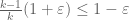$\frac{k-1}{k} (1+\varepsilon) \leq 1-\varepsilon$ , which comes out to $\varepsilon \sim 1/2k$ . After that, the cost of increasing epsilon starts creeping up, and eventually exceeds the marginal profit of expanding the support of F, and it does seem plausible to me that the crossover occurs for epsilon near 1/k. I’ll try to see if there is some formal way to make this precise (e.g. by generalising the upper bound 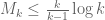$M_k \leq \frac{k}{k-1} \log k$ to an upper bound on $M_{k,\varepsilon}$ which peaks for $\varepsilon$ comparable to 1/k).

13 February, 2014 at 5:33 pm

Aubrey de Grey

Terry, can this kind of argument also explain the dependence of the optimal epsilon on d for a given k?

15 February, 2014 at 9:25 am

Eytan Paldi

A simple partition for $M_{k,\epsilon}$ computation:

$F$ is supported on $R = (1+\epsilon) \mathcal R_k$ .

The functional $J^{(i)}(F)$ is determined by $F$ values over

$A := (1-\epsilon) \mathcal R_{k-1}$

and the domain $B_i$ which is determined by

$s_i \leq 1-\epsilon ; 1-\epsilon < t_i \leq 1+\epsilon - s_i$

where $s_i := \sum_{j \neq i} t_j$ .

Let $B := \cup_i B_i$ and

$C := R \setminus (A \cup B)$ .

Since the numerator $J(F)$ is independent on the values of $F$ on $C$ , it follows that the optimal $F$ should vanish on $C$ (i.e. optimal $F$ is supported on $A \cup B$ ).

My suggestion therefore is to optimize $F$ as a piecewise polynomial supported on the $k+1$ domains

$A, B_1, ... , B_k$

In fact, only the polynomial representation of $F$ over $A, B_1$ are needed – using $F$ symmetry (it should be remarked that the polynomial representation of $F$ on $B_1$ is not(!) necessarily symmetric).

Remark: Since the optimal $F$ vanishes over $C$ , it follows that it can't be real analytic (and, in particular, polynomial) on $R$ – explaining its slow convergence when represented by a single polynomial.

15 February, 2014 at 10:37 am

Eytan Paldi

There is a problem in my suggestion above: in the definition of $B_i$ above, the lower bound for $t_i$ should be $1-\epsilon -s_i$ , but now the domains $B_i$ are not necessarily disjoint (so perhaps further decomposition is necessary).

15 February, 2014 at 12:17 pm

Eytan Paldi

The simplest improvement is to use a single symmetric polynomial approximation for $F$ on $A \cup B$ with $F=0$ on the remaining $C$ . The resulting improvement is by computing the denominator $I(F)$ over $A \cup B$ – without the (unnecessary) current contribution from the remaining region $C$ .

15 February, 2014 at 3:11 pm

Terence Tao

I managed to make a little bit of headway in clarifying the relationship between the lower bounds on $M_k$ (or $M_{k,\varepsilon}$ coming from choosing good functions F, to the upper bound $M_k \leq \frac{k}{k-1} \log k$ that one gets from Cauchy-Schwarz. One can abstract the Cauchy-Schwarz argument as follows: whenever one has a function $G: {\cal R}_k \to {\bf R}^+$ which symmetrises to 1 (or to something bounded above by 1), we have the bound

$M_k \leq k \sup_{t_1+\dots+t_{k-1} \leq 1} \int_0^{1-t_1-\dots-t_{k-1}} \frac{dt_k}{G(t_1,\dots,t_k)}.$ (*)

Indeed, given any F on ${\cal R}_k$ , we get from Cauchy-Schwarz that

$\int_{t_1+\dots+t_{k-1} \leq 1} (\int_0^{1-t_1-\dots-t_{k-1}} F\ dt_k)^2\ dt_1 \dots t_{k-1}$
$\leq X \int_{{\cal R}_k} G(t_1,\dots,t_k) F(t_1,\dots,t_k)^2\ dt_1 \dots t_k,$

where X is the supremum appearing in (*), and the claim then follows from symmetrising.

By taking $G(t_1,\dots,t_k) = 1 + (k-1) t_k - t_1 - \dots - t_{k-1}$ (which symmetrises to 1) we obtain the standard bound $M_k \leq \frac{k}{k-1} \log k$ .

On the other hand, if we have an eigenfunction

$M_k F(t_1,\dots,t_k) = \sum_{j=1}^k \int F(t_1,\dots,t_{j-1},t,t_{j+1},\dots,t_k)\ dt$

with F positive, then we can take

$G(t_1,\dots,t_k) := k \frac{\int F(t_1,\dots,t_{k-1},t)\ dt}{M_k F(t_1,\dots,t_k)},$

which symmetrises to 1, and obtain equality in (*). So this shows that Cauchy-Schwarz can in fact give optimal bounds if one chooses G correctly.

As such, if we wanted to, we could try to numerically improve the upper bound $M_k \leq \frac{k}{k-1} \log k$ by experimenting with other G than $1 + (k-1)t_k - t_1 - \dots - t_{k-1}$ that symmetrise to 1. Unfortunately, this is a nonlinear optimisation problem and not so easily settled by quadratic programming, as is the case with the lower bounds.

A similar story happens for $M_{k,\varepsilon}$ , where G is now supported on $(1+\varepsilon) \cdot {\cal R}_k$ and the analogue of (*) is

$M_{k,\varepsilon} \leq k \sup_{t_1+\dots+t_{k-1} \leq 1-\varepsilon} \int_0^{1-t_1-\dots-t_{k-1}+\varepsilon} \frac{dt_k}{G(t_1,\dots,t_k)}.$

Again, this bound is sharp if we have a positive eigenfunction at $M_{k,\varepsilon}$ and G is chosen appropriately. Taking G of the form

$G = 1 + a ((k-1)t_k - t_1 -\dots - t_{k-1})$ (**)

for some parameter $\frac{1}{1+\varepsilon} \leq a \leq \frac{1}{1-\varepsilon}$ that one is free to choose, one concludes the bound

$M_{k,\varepsilon} \leq \frac{k}{a(k-1)} \log( k + \frac{(a(1+\varepsilon)-1)(k-1)}{1-a(1-\varepsilon)} ).$

If one takes $a=1/(1+\varepsilon)$ one recovers the crude bound 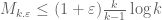$M_{k.\varepsilon} \leq (1+\varepsilon) \frac{k}{k-1} \log k$ . If one takes $a=1$ , one instead gets the bound 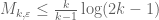$M_{k,\varepsilon} \leq \frac{k}{k-1} \log(2k-1)$ , which is slightly better for large epsilon. One could optimise in a to see what else one could get, but I suspect that one could do even better by playing with more general weight functions than (**).

2 March, 2014 at 6:42 pm

Eytan Paldi

It should be remarked that the last bound (with $a =1$ ) is already optimal! to see that, let (for fixed $k$ and $\epsilon \in (0, 1)$ denote for $a\in [\frac {1}{1+\epsilon}, \frac {1}{1-\epsilon})$ by $f(a)$ the above upper bound for $M_{k, \epsilon}$ . Since

$f(a) = k \int_0^{2 \epsilon} \frac {1}{1+a[(k-1)t-(1-\epsilon)]} d t$

It follows (e.g. by taking derivatives under the integral sign) that $f$ is convex (and therefore has a minimum at $a=1$ if $f '(1) = 0$ .
It remains only to find $\epsilon \in (0, 1)$ for which $f '(1) = 0$ .
A simple calculation shows that $f '(1) = 0$ for

$\epsilon = \frac {2 k - 2}{(2 k - 1) \log (2 k - 1)}$

Remark: this $\epsilon$ is quite large! ( $O(1/ \log k)$ ).

3 March, 2014 at 6:41 pm

Eytan Paldi

A simple lower bound on $\epsilon$ :

Suppose that $M_{k, \epsilon} > 4$ for some $k, \epsilon$ .
Hence (by the crude bound above – with $a = 1/(1+\epsilon)$ )

$(1+\epsilon)\frac {k}{k-1} \log k > 4$ , i.e.

$\epsilon > \frac {4(k-1)}{k \log k} - 1$

Examples:

$k = 50$ : $\epsilon > 0.00203$
$k = 49$ : $\epsilon > 0.00682$
$k = 48$ : $\epsilon > 0.01174$
$k = 47$ : $\epsilon > 0.01681$
$k = 46$ : $\epsilon > 0.02204$
$k = 45$ : $\epsilon > 0.02743$
$k = 40$ : $\epsilon > 0.05723$
$k = 35$ : $\epsilon > 0.09292$
$k = 30$ : $\epsilon > 0.13685$

Remark: these (somewhat crude) numerical bounds show that $\epsilon$ can be much larger than expected!

18 March, 2014 at 5:23 am

Eytan Paldi

Let $F_0$ be positive and square integrable on $\mathcal R_k$ .

By taking (for $i = 1, ... , k$ )

$G_i := \mathcal L_k^{(i)} F_0 / F_0$

We get $\sum_i G_i = \mathcal L_k F_0 / F_0$ , and

$\mathcal L_k^{(i)} (1/G_i) = 1$

Which (by the above C-S bounding argument) gives the simple bound

$M_k \le || \mathcal L_k F_0 / F_0 ||_{\infty}$ (1)

Remarks:

1. The bound (1) may be generalized (for $F_0$ not necessarily positive) by taking the supremum norm over the support of $F_0$ .

2. This upper bound should be good for $F_0$ sufficiently close to an eigenfunction of $\mathcal L_k$ (e.g. using $F_0$ giving good lower bound for $M_k$ ).

3. If $F_0$ is an eigenfunction of $\mathcal L_k$ with corresponding eigenvalue $\lambda$ , the bound (1) shows that
$M_k \leq \lambda$ – implying that $\mathcal L_k$ has at most one(!) eigenvalue (which must be $M_k$ ).

4. It seems that the above upper bound derivation can be generalized for $M_{k, \epsilon}$ .

29 March, 2014 at 12:26 pm

Eytan Paldi

Remark 3 above gives a very simple proof that the exact expression found for the (necessarily single) eigenvalue of $\mathcal L_2$ is in fact its norm $M_2$ .

15 February, 2014 at 3:36 pm

Eytan Paldi

The last upper bound shows that

$M_{23, \epsilon} \leq 3.9796 ... < 4$

Implying (using this M-value) $k \geq 24$ .

17 February, 2014 at 9:12 am

Pace Nielsen

With $d=16$ we have $M_{53,1/35}\approx 4.000161$ . It turns out $\varepsilon=1/35$ is optimal for degree 16 polynomial approximations. (Each individual run takes about 11 hours, and I started at 1/40, so it took all weekend to find this value.)

I still have no feeling about the relationship between larger epsilon, larger degrees of polynomial approximation, and corresponding improvement in the M computation. I’m running the $k=52,d=18$ computation now; I expect each individual run to take about a week.

17 February, 2014 at 9:19 am

Aubrey de Grey

Great job Pace. Perhaps a good way to obtain a better guess for the best d and epsilon for k=52 might be first to identify those values for k=54 and 55, which if I understand you you can determine relatively rapidly?

17 February, 2014 at 9:52 am

Pace Nielsen

Unfortunately, it takes just as long to find the optimal epsilon for other values of k. As for the best d, I’m getting close to the limit imposed by RAM issues, as well as run-time issues.

17 February, 2014 at 9:59 am

Aubrey de Grey

Apologies, I was unclear – what I meant was that as k increases one reaches M=4 with smaller degree and also smaller epsilon, and I think you said that execution time is very dependent on both d and epsilon even if not on k. (Right?) I was thinking therefore that if we knew the smallest d for which M_54, M_55 etc can top 4, and the corresponding best epsilon for those k and d, we might be able to extrapolate reasonably accurately to what d and epsilon to try first for k=52.

17 February, 2014 at 11:50 am

Pace Nielsen

I see what you mean now. Given that d=18 is already at the limit of my computing power there was no real need to try and extrapolate what degree was best; but it did look like d=18 had a decent chance of succeeding.

As for extrapolating epsilons, I started with $\varepsilon=1/33$ as that seems to be a reasonable improvement when increasing the degree by 2. (The difference between 1/35 and 1/34 when d=16 was quite small, so even if this isn’t optimal it shouldn’t hurt us much.)

17 February, 2014 at 11:15 am

Eytan Paldi

This improves H to 264!

In order to get faster convergence we need to use the fact that the optimal $F$ is supported only(!) on the region over which the integrands of the numerator functionals $J^{(i)}_{k, \epsilon}(F)$ are integrated.

Therefore $F=0$ on the remaining region – (as in the case of region $D$ with $FD = 0$ in the computation of $\hat M''_{3, 1/4, 1}$ ) – leading to discontinuities on the boundary of the support – resulting by very slow convergence when trying to approximate $F$ by a single polynomial over the whole region $(1+\epsilon) \mathcal R_k$ .

The simplest solution is to compute the denominator functional $I(F)$ over the reduced support of $F$ (used in the numerator computation).

17 February, 2014 at 11:59 am

Pace Nielsen

It may be possible to come up with a formula for the integral of a monomial over this region, similar to what James does in his paper. This is definitely something we should look at.

17 February, 2014 at 1:03 pm

Eytan Paldi

The reduced support of $F$ is the union of the regions
$D_i$ on which the integrands of the numerator functionals
$J^{(i)}_{k, \epsilon}$ are integrated. Each $D_i$ is determined by

$\sum_j t_j \le 1+\epsilon ; \sum_{j \neq i} t_j \le 1-\epsilon$ .

Therefore $F = 0$ on the remaining region determined as the intersection of the $k$ half spaces

$(t_1, ... , t_j) : \sum_{j \neq i} t_j > 1-\epsilon ; i = 1, ... , k$

and the whole region $(1+\epsilon) \mathcal R_k$ .

Therefore the remaining region is a convex polytope (on which it is perhaps easier to integrate its contribution to $I(F)$ – to be subtracted from the present value of $I(F)$ contributed by the whole region $(1+\epsilon) \mathcal R_k$ ).

17 February, 2014 at 7:28 pm

Terence Tao

Great news! I’ll update the wiki accordingly.

One amusing consequence of this calculation is that we now have a divergence between the H_2 bound on GEH, and the H_1 bound unconditionally. We now have $H_1 \leq 264$ unconditionally, but on GEH we still only have $H_2 \leq 270$ ; the value $\varepsilon=1/35$ is inadmissible for the GEH calculation because it is larger than $1/(k-1)$ .

18 February, 2014 at 6:40 am

Pace Nielsen

That is fun fact! I imagine that it might be possible to get $H_1\leq 264$ with $\varepsilon=1/52$ by using even higher degree approximations, but I doubt we could continue such jerry-rigging indefinitely. In particular, I think we have a good chance to get $k=52$ (or even $k=51$ ), but not with $\varepsilon=1/(k-1)$ .

17 February, 2014 at 1:56 pm

Aubrey de Grey

I’ve had a go at developing some extensions to Pace’s k=3 code (learning Mathematica as I go) that I hope may also be useful for two-digit k. My starting point is the suspicion that we can cut down the number of monomials included in the various polynomials quite considerably without impacting M very much, just by finding variables that can be set to zero with little impact. If that’s true, we might be able to develop a more systematic way to select monomials than the essentially serendipitous approach (e.g. Pace’s selection of only monomials with even total degree). The algorithm I’ve so far developed is pretty clunky and wouldn’t really scale, but it can certainly be streamlined.

I also added a system for simplifying the coefficients once the minimal set of monomials has been found: rather than normalising the eigenvector to the first variable (AA1) as Pace as doing, I mormalise the error in the Rationalize function to 1/2, thus making all the elements integers, and find the smallest multiple of the eigenvector that keeps M above 2. (This is actually more laborious than it sounds because, as might be expected from what Rationalize does, M does not vary remotely monotonically with the multiplier.) With this approach I can get the number of monomials down to 81 using the degree set G=U=4,A=C=2,B=E=H=S=T=1, with the following polynomials:

FA = -21 + 27 x – 17 x^2 + 24 y – 16 x y – 15 y^2 + 26 z – 12 x z – 9 y z – 17 z^2

FB = -9 + 6 x + 11 y + 2 z

FC = -7 + 14 x – 10 x^2 + 12 y – 11 x y – 8 y^2

FE = -2

FG = 6075420501/346240 – (16675800469 x)/173120 + 155635 x^2 – (6686927443 x^3)/64920 + 24572 x^4 – (9395259281 y)/86560 + (33229279693 x y)/81150 – (21832401219 x^2 y)/54100 + (5005953883 x^3 y)/40575 + (4054772621 y^2)/27050 – (38485294907 x y^2)/108200 + (86436312 x^2 y^2)/541 – (7063782421 y^3)/81150 + (3417366154 x y^3)/40575 + 24572 y^4 – (3180108497 z)/69248 + (124261104937 x z)/649200 – (90238133481 x^2 z)/432800 + (5649716833 x^3 z)/81150 + (142158687241 y z)/649200 – 556968 x y z + (3753280304 x^2 y z)/13525 – (88739020157 y^2 z)/432800 + (6718761079 x y^2 z)/27050 + (2430958652 y^3 z)/40575 + (1164494227 z^2)/25968 – (27311867067 x z^2)/216400 + (940600277 x^2 z^2)/13525 – (1983863621 y z^2)/13525 + (5100751699 x y z^2)/27050 + (3775389779 y^2 z^2)/54100 – (5026420987 z^3)/259680 + (4481310893 x z^3)/162300 + (1323771941 y z^3)/40575 + (101101127 z^4)/32460

FH = 2

FS = 0

FT = -(9/2) + 3 x + 6 y + 3 z

FU = -(53425823/20480) + 15471 x – 13354 x^2 – 25893 x^3 + 24572 x^4 + 12 y – (3119 x^2 y)/100 – (300147 y^2)/1280 + 5974 z – 34366 x z + (26850499 x^2 z)/800 + 7933 x^3 z + (789 y^2 z)/2 – (5615871 z^2)/1280 + 23540 x z^2 – 15951 x^2 z^2 – 180 y^2 z^2 + 952 z^3 – 4934 x z^3 + 60 z^4

The hope here is that a pattern can be discerned for which monomials can be most cheaply thrown out. If such a pattern emerges for small k and d, maybe it can indicate how enough of them might be eliminated from the outset for larger k and d to allow acceptable computational efficiency at the least cost in M. Presumably the place to start is with R or R’ rather than any domain that needs partitioning – at least until there is an implementation of Terry’s proposal for the simplex of size 2.

17 February, 2014 at 2:36 pm

Eytan Paldi

It is perhaps possible to reduce this number of coefficients by locating the smallest coefficients (or the “less important” coefficients, using trial & error) and imposing more vanishing constraints for them, and see if the resulting M-value is still above 2.

17 February, 2014 at 6:30 pm

Aubrey de Grey

Yes, that’s exactly what I did. One thing I didn’t make clear is that the saving achieved in this way rises pretty rapidly as M is allowed to fall below what can be achieved at higher degree with all monomials used. I think the best M achieved so far with degrees as large as 5 (and 306 possible monomials) is only 2.0012, so staying above 2 with only 81 monomials seemed like a good sign. As a further data point I just looked more at the behaviour with constant degree (which is presumably the setting relevant to larger k). When all nine degrees are set to 2, allowing 90 monomials in principle, the best M is 1.9983, and when they are set to 3, which as I noted earlier allows M=2.0000339 using all possible monomials, we can reach M=1.9983 with only 96 monomials out of the possible 180 (and the actual 136 needed to reach M=2). M=1.96 can be reached using degree 3 with only 23 monomials! (All this is with epsilon=1/4 and dropping M6 and M8, by the way.)

Given this rather encouraging trend, I now plan to be more systematic than my previous intention to try to discern patterns: instead I plan to explore slowly introducing monomials of progressively higher total degree and number of dimensions featuring, while continuing to exclude monomials already eliminated in previous rounds. I’m fairly optimistic that this can be used in non-geological execution time for k quite a bit larger than has been explored thus far using all monomials.

17 February, 2014 at 3:15 pm

interested non-expert

I find the result of H_1<=6 on GEH very interesting, especially the proof that its optimal for sieve-theoretic methods. Now I wonder what would be – in a strange mathematical universe – the implications of H_1==6 (instead of 2 or 4)?
I'm thinking of implications that could be proven right or wrong, thus providing an alternative route to answere this question.

Thanks alot for your answere and good luck with continueing on unconditional H_1! (I'm following your research here on a daily basis, and i'm superexcited about every progress :-) )

18 February, 2014 at 3:17 pm

Terence Tao

This would indeed be an odd mathematical universe – assuming GEH, what it would mean is that there is a “conspiracy” between n and n+2, in that whenever these two numbers are both almost prime (in the sense of having no small prime factors), and one has an odd number of prime factors, then the other will almost always have an even number of prime factors (and vice versa). Similarly for n and n+4. (This doesn’t lead to a contradiction, because n, n+2, n+4 cannot all be almost prime at once, seeing that one of these numbers is necessarily divisible by 3.) This is extremely unlikely, but thus far we don’t seem to have any viable route to force a true contradiction out of this. (In a similar vein, it is incredibly unlikely that the digits of pi start exhibiting patterns such as alternating between odd and even numbers after some finite point, but we don’t know how to deduce a contradiction from such a bizarre scenario.)

19 February, 2014 at 2:22 am

Michel Eve

I have a question regarding the value of the proof that H1 is less or equal to 6 under GEH. I understand that any progress on H1 unconditionnaly is a major step forward but why is a progress under GEH so important ? Is it because GEH is potentially easier to prove than the twin prime conjecture ? Can it be a step towards proving GEH ? For a non expert the use of an other conjecture to work towards the proof of a main conjecture is always puzzling….

19 February, 2014 at 8:52 am

Terence Tao

Yes, I would consider GEH as being closer to being provable than, say, the twin prime conjecture. One can very roughly gauge the complexity of a sum in analytic number theory by how many references it makes to a complicated arithmetic function, such as the von Mangoldt function $\Lambda$ . (There are other important measures of complexity, such as the amount of usable averaging present in the sum, or the level of accuracy one demands on the sum, but I will ignore these other dimensions of complexity for the purposes of this comment.) For instance, the sum $\sum_{x \leq n \leq 2x} 1$ involves no such functions and is very easy to compute; the sum $\sum_{x \leq n \leq 2x} \Lambda(n)$ involves one such function and requires the prime number theorem to evaluate accurately. The twin prime conjecture is associated with the sum $\sum_{x \leq n \leq 2x} \Lambda(n) \Lambda(n+2)$ , which involves two separate occurrences of $\Lambda$ and which we cannot yet evaluate accurately (although we do have some upper bounds). EH involves sums such as $\sum_{x \leq n \leq 2x: n = a\ (q)} \Lambda(n)$ (or more precisely, certain averaged, renormalised versions of this sum) and is thus in principle on the same basic level of difficulty as the prime number theorem (and indeed results similar to the PNT, such as the Siegel-Walfisz theorem, are used in the proof of partial versions of EH such as the Bombieri-Vinogradov theorem). GEH has a similar story, but with $\Lambda$ replaced by a more general arithmetic function (but still one of comparable complexity to $\Lambda$ ).

Also, one can view things the other way around: each time one shows an implication of the form “Conjecture X implies Conjecture Y”, one obtains some more clarity and insight as to the relative level of difficulty of the two conjectures. In this case, it shows that despite superficial similarities, the $H_1 \leq 6$ conjecture and the $H_1 = 2$ conjecture (i.e. the twin prime conjecture) have quite different levels of difficulty; we now know the former is much easier in that it is reducible to a “one arithmetic function” problem, namely GEH, whereas the latter seems to be an almost irreducible example of a “two arithmetic function” problem, which is still largely beyond our current methods.

It’s also worth noting that these arguments don’t just give $H_1 \leq 6$ from GEH, but also give a bunch of other results as well. For instance, as noted recently here, we now know that GEH implies that _either_ the twin prime conjecture is true, _or_ the even Goldbach conjecture is asymptotically true up to an error of 2 (or both). One could imagine GEH eventually acquiring a status similar to GRH, which also has a large number of seemingly unrelated analytic number theory consequences which would follow from its resolution, and is now a central open problem in the subject.

Finally, it should be noted that Zhang’s most important technical achievement was his establishment of a certain restricted fragment of the Elliott-Halberstam conjecture that goes beyond what was previously known (i.e. Bombieri-Vinogradov theorem, together with some even more restricted fragments of EH from the work of Bombieri, Fouvry, Friedlander, and Iwaniec and later authors.) While Zhang’s work (or the numerical improvements to it in Polymath8a) are still quite far from a full resolution of EH or GEH, it does give us some hope that this conjecture is not utterly intractable. (Twin primes, on the other hand, are another story, as we have not made any serious dent in the parity barrier that guards this conjecture yet, although this barrier has been circumvented in some other contexts in which more averaging is present, so it is not completely hopeless.)

18 February, 2014 at 7:46 pm

Anonymous

I guess that its worth recalling a comment from a few weeks ago now we have shown $H_1$ is at most 6 under GEH.

Under GEH, at least one of the following is true;
1. There are infinitely many twin primes
2. Every large even integer $N$ is within 2 of a number which is the sum of 2 primes.

Therefore, if we do live in a bizarre world where there is a conspiracy preventing n and n+2 both being prime, we can almost prove the Goldbach conjecture (under GEH).

18 February, 2014 at 3:08 pm

Terence Tao

I’ve just been contacted by a senior employee at Dropbox, who has kindly offered some additional space for users of the Polymath dropbox folder (from 2GB to 10GB) as a gesture of support for our project. At present I don’t think we actually need this amount of space (the folder currently takes up just 0.02 GB of space), but it is conceivable that we might have some future need (e.g. if some of Pace’s monster-memory computations can somehow be parallelised). Anyway, this is something to keep in mind in case shared disk space somehow becomes the bottleneck.

18 February, 2014 at 6:22 pm

Pace Nielsen

I googled “parallel matrix inversion” and was led to the package LAPACK http://www.netlib.org/lapack/ It looks like this might do the trick if we want to try do parallelize our computations.

18 February, 2014 at 6:49 pm

Terence Tao

Perhaps the “cheapest” parallelisation one could do is simply to put (a copy of) the active code and data folder on Dropbox, and let different people try different values of k, different values of epsilon, etc. There might be a little bit of data sharing one could do; for instance, when keeping k fixed and trying different values of epsilon, one could rescale by 1+epsilon so that all polynomials are supported in the same simplex ${\cal R}_k$ , which means that the matrix for the I-functional is common to all choices of epsilon and only needs to be computed once. (But this is probably not the bottleneck; the J-functional is much more complicated. But perhaps one could precompute the inverse of I or whatever it is that is needed in the quadratic program.)

18 February, 2014 at 6:55 pm

comment

I haven’t been following this project closely, but are you doing numerical (e.g. 64 bit floating point numbers) matrix inversion *without* lapack? The more explicitly parallel version of lapack is scalapack http://www.netlib.org/scalapack/

18 February, 2014 at 8:01 pm

Pace Nielsen

To this point we’ve been doing exact arithmetic in Mathematica. (Regarding the linear algebra, one step is an explicit matrix inversion, and the next is finding a floating point approximation for the largest eigenvector.)

18 February, 2014 at 8:21 pm

comment

Is recent code anywhere? I don’t know anything about prime numbers or number theory, but I might help with applied linear algebra and numerical nonlinear optimization. If you care about extreme eigenvectors why bother explicitly inverting the matrix first? I’m sure I’m missing something..

18 February, 2014 at 8:27 pm

Eytan Paldi

I don’t understand why a matrix inversion is needed (in order to show that there is a vector $x$ for which $x^{T}B x > 4 x^{T}A x$ , it is equivalent that $B - 4 A$ has a positive eigenvalue.

18 February, 2014 at 8:40 pm

Pace Nielsen

This was part of the code that I simply copied directly from James’ earlier code, but my impression for the reason for the matrix inversion is so that we can find explicit lower bounds for $M_k$ (i.e. we don’t know, a priori, what constant $c$ we can use to force $B-cA$ to have a positive eigenvalue). [It is also a sanity check that things are working correctly. I just did a separate computation where the matrix was not invertible; and I’m still trying figure out where in my code I made a mistake.]

18 February, 2014 at 8:54 pm

Eytan Paldi

$M_k$ is the largest eigenvalue of the generalized eigenvalue problem $(B - \lambda A) x = 0$ . There is an efficient algorithm to find the generalized eigenvalues and eigenvectors of the pair $(A, B)$ without(!) matrix inversion (as I already mentioned in a previous comment) – see e.g. the wikipedia article on matrix pencils.

18 February, 2014 at 8:58 pm

Pace Nielsen

@comment: The linear algebra problem is described on page 20 of Maynard’s paper http://arxiv.org/pdf/1311.4600v2.pdf, and is the following: Given real, symmetric positive definite matrices $M_2,M_1$ (with $M_1$ invertible) find a vector $a$ maximizing the quotient $(a^{T}M_2 a)/(a^{T}M_1 a)$ . This is currently being done by finding $M_1^{-1}$ , then finding an (approximation to an) eigenvector $a$ of $M_{1}^{-1}M_2$ with largest eigenvalue.

It would also be sufficient to merely prove there exists a vector for which that quotient is bigger than 4. However, the actual value of the maximal quotient is helpful in other ways, such as helping us fix certain constants, it gives an intuition about how the quotient is behaving, etc…

18 February, 2014 at 9:00 pm

Pace Nielsen

@ Eytan: Yes, I remember your earlier post! I looked into the function you linked to, and it is not currently implemented in Mathematica. Hopefully something similar is implemented in one of these other programs being currently discussed.

18 February, 2014 at 10:10 pm

comment

Yes this is the generalized eigenvalue problem. Here’s a python example with four ways to solve it, plus output. I’m sure Mathematica, Matlab, etc. have similar implementations. Sorry for spamming it up, feel free to delete or move.

“””

http://docs.scipy.org/doc/scipy/reference/generated/scipy.sparse.linalg.eigsh.html

“””
from functools import partial

import numpy as np

from scipy.linalg import inv, eigh, eig, norm
from scipy.sparse.linalg import eigsh
from scipy.optimize import minimize

def normalized(x):
return x / np.linalg.norm(x)

def sample_matrix(n, s):
A = np.random.randn(n, n)
A = np.dot(A, A.T)
A = np.trunc(s*A)/s
return A

def generalized_rayleigh_ratio(A, B, x):
x = normalized(x)
return x.dot(A).dot(x) / x.dot(B).dot(x)

def objective(A, B, x):
disambig = np.square(1 – norm(x))
return disambig – generalized_rayleigh_ratio(A, B, x)

def main():
n = 4
s = 1e3
A = sample_matrix(n, s)
B = sample_matrix(n, s)
f = partial(objective, A, B)
result = minimize(f, np.ones(n), method=’bfgs’)
wa, va = eigsh(A, 1, B)
wb, vb = eig(np.dot(inv(B), A))
wc, vc = eigh(A, B, eigvals=(n-1, n-1))
print ‘A:’
print A
print
print ‘B:’
print B
print
print ‘eigsh:’
print wa[0]
print normalized(va[:, 0])
print
print ‘eig:’
print wb[0]
print normalized(vb[:, 0])
print
print ‘eigh:’
print wc[0]
print normalized(vc[:, 0])
print
print ‘optimization:’
print generalized_rayleigh_ratio(A, B, result.x)
print result.x
print

main()

—-

A:
[[ 1.115 0.869 0.656 0.501]
[ 0.869 5.201 1.734 -0.535]
[ 0.656 1.734 1.337 -0.132]
[ 0.501 -0.535 -0.132 0.554]]

B:
[[ 3.693 -0.663 0.265 -0.206]
[-0.663 1.708 0.021 0.281]
[ 0.265 0.021 0.72 -0.289]
[-0.206 0.281 -0.289 1.253]]

eigsh:
4.38071133898
[ 0.16613191 0.7780925 0.59849769 -0.09366305]

eig:
(4.38071133898+0j)
[ 0.16613191 0.7780925 0.59849769 -0.09366305]

eigh:
4.38071133898
[-0.16613191 -0.7780925 -0.59849769 0.09366305]

optimization:
4.38071133898
[ 0.16613202 0.77809265 0.59849769 -0.09366297]

19 February, 2014 at 9:30 am

Eytan Paldi

It should be remarked that the exact matrix inversion has the drawback that the elements of the inverse matrix have very large denominators – (whose number of digits may be the order of the matrix size!) – requiring very large memory – which may explain the very slow computation!

18 February, 2014 at 7:29 pm

James Maynard

I think in principle this problem should be fairly ameanable to parallization, if we decide that is the next step.

The calculation of individual entries in the matrices are more-or-less independent, and can easily be calculated on separately.

For the eigenvalue step, a sufficient proof that $M_1^{-1}M_2$ has an eigenvalue which is bigger than 4 is that the determinant of $4M_1-M_2$ is negative. I think this should probably be parallelizale using e.g. the chinese remainder theorem (and I believe there is a large amount of literature on calculating large determinants).

18 February, 2014 at 8:05 pm

Eytan Paldi

A necessary and sufficient condition is that $4 M_1 - M_2$ has a positive eigenvalue. (which is not implied by a negative determinant!)

18 February, 2014 at 8:18 pm

Eytan Paldi

Correction: In my comment above it should be $M_2 - 4 M_1$ (instead of $4 M_1 - M_2$ ).

18 February, 2014 at 8:18 pm

Pace Nielsen

To help implement the calculation of individual entries, we may also want to create a large look-up table for the structure constants that arise when we multiply elements of our basis. I haven’t thought much about this issue (because you had that excellent idea which doubled the degrees which had made it moot at the time), but I recall Terry had some ideas along those lines.

19 February, 2014 at 8:37 am

Pace Nielsen

I’ve uploaded my code for the k=53 computation to the Polymath8b dropbox. People are free to play around with it (if they have Mathematica). Some changes/things that should be done are the following:

1. Currently I have not imposed the (necessary) restriction that signatures should have length at most k, because the degree has never been big enough to make a difference.

2. My function for computing structure constants when multiplying elements of the basis is extremely slow and RAM intensive for large signatures. This should be fixed, perhaps along the lines Terry suggested earlier.

3. We should find a way to transfer the linear algebra portion to a better setup than Mathematica, that could possibly be parallelized.

4. Someone should double check that my computations are actually giving the correct values! (If we do parallelize this, we probably just want to rewrite the code from scratch in any case.)

19 February, 2014 at 2:04 pm

Pace Nielsen

By the way, I’m happy to run these computations on the BYU supercomputers if it looks like that will help. Before I go to the trouble of figuring out how to install and run LAPACK, it would be good to get confirmation that this program is the best one to do the generalized eigenvalue problem on very large sized (at least 1500 x 1500) rational (although we could use floating point approximations) symmetric matrices.

19 February, 2014 at 3:06 pm

comment

I looked at Maynard’s code in the dropbox and those 42×42 matrices are dense with entries spanning more than 20 orders of magnitude and have condition numbers >1e30 which may pose challenges to straightforward application of the double precision LAPACK (or more appropriately ARPACK) library functions. Maybe it would be OK but I see that as a possible red flag. It will not do rational arithmetic. Everything else equal, large N=1500 matrix sizes should not be a problem because I think you could solve the optimization without doing anything like N^3 (no inversion, no matrix-matrix multiplication).

By the way I would be surprised if Mathematica does not already have LAPACK/ARPACK baked into it somehow. In Mathematica terms these libraries use MachinePrecision http://reference.wolfram.com/mathematica/ref/MachinePrecision.html

19 February, 2014 at 4:58 pm

IIIIIIIIIIIII

Indeed Mathematica does use LAPACK. https://reference.wolfram.com/mathematica/tutorial/LinearAlgebraMatrixComputations.html

19 February, 2014 at 5:57 pm

Pace Nielsen

Thanks! The function “GeneralizedEigenvector” is no longer supported, but it appears that the functionality is still there within the usual “Eigenvector” function. I’ve tested it a bit, and it looks quite good so far.

20 February, 2014 at 4:07 am

foobar

Mathematica uses LAPACK numerics, but this doesn’t imply it’s limited to “machine precision” (that is, “doubles”). Mathematica also supports arbitrary precision reals with LAPACK. (This is mentioned on the page.) This is, no doubt, considerably slower, but extra numerical precision is available, and you are not really left to the mercy of precision supported by “double-precision” floats.

20 February, 2014 at 8:14 am

comment

As Pace mentions, the Mathematica Eigenvector function will do generalized eigendecomposition. Here’s the modification of the last bit of Maynard’s dropbox code that gets the same ratio.

ev = Eigenvectors[{N[M2, 150], N[M1, 150]}, 1][[1]];
rv = Rationalize[ev, 10^-40];
Ratio = k*(rv.M2.rv)/(rv.M1.rv);
N[Ratio, 20]

4.0020697619380471369

Some points are that Mathematica will do generalized eigenvector decomposition with more-than-machine precision (as foobar mentions), and that this formulation uses neither exact matrix inversion (as opposed to Maynard’s code) nor floating point matrix inversion nor matrix-matrix multiplication, so it should be fast. I have a hard time following the newer codes on the dropbox but presumably this modification could be applied there as well.

20 February, 2014 at 12:12 pm

Pace Nielsen

I started testing the Mathematica functionality for solving the generalized eigenvector problem, and ran into what I hope is a small problem. We first compute the dense rational symmetric matrices corresponding to the I and J integrals. (I’m working on speeding up this step along the lines Terry outlined a while ago, but this might take a while as I have a few other projects on my plate.) We then have to use real approximations of these matrices since Mathematica doesn’t do the generalized eigenvector solving on rational matrices.

What I need to know is the best way to take real approximates of the matrices but still get the largest eigenvalue correct to (say) the first five decimal places. (I can do as in Comment’s code, and take Eigenvectors [{N[M2,*], N[M1,*],1] where * is a large number; but this has the potential to slow down the computation more than is necessary.)

20 February, 2014 at 12:46 pm

comment

The current code which uses the exact inverse also uses Eigenvectors[N[M, *], …] where * is a large number, so would the accuracy concern not apply to both the current method and the proposed generalized eigenvalue method?

In Maynard’s code I noticed that the entries of the matrices M1 and M2 both decrease in magnitude from the upper left towards the lower right, and that the condition number can be improved by left- and right- multiplying by a diagonal scaling matrix. Maybe tricks that use this diagonal scaling could help with the numerical stability, if Mathematica is not already doing something like this internally?

20 February, 2014 at 12:56 pm

Pace Nielsen

@comment: Sorry I wasn’t clear! It is not accuracy, per se, that I’m concerned with. Rather it is *quick* accuracy. If taking 150 digit approximations of the matrices is the quickest way to get get 5 digit accuracy in the eigenvalue, so be it. But I’m hoping there is a better way.

20 February, 2014 at 1:35 pm

comment

In a related but slightly different question, if you get a proposed rational vector then it is easy to use Mathematica to decide if its associated ratio is greater than or less than 4?

20 February, 2014 at 1:46 pm

Pace Nielsen

Yes. Given a potential vector it is quite easy to compute the corresponding ratio. Put another way, the last 3 lines of the code you posted run fairly quickly. [There may be some room for improvement, but it isn’t currently the hangup.]

20 February, 2014 at 2:48 pm

comment

Regarding the amount of precision of the two input matrices needed for a target precision for the max generalized eigenvalue, I guess a full answer would involve something like a ‘generalized eigenvalue problem condition number’ which I don’t know how to do. Googling shows that Maple and MATLAB have possibly related functions named EigenConditionNumbers and condeig.

On the other hand, a half-answer is easy because if low precision matrices give you a candidate rational vector whose associated ratio is > 4 then you are done.

For Maynard’s example the problem seems strangely stable. For example lowering the precision by changing N[M, 150] to N[M] gives a ratio that is equal to >12 places, even though the input matrices are badly conditioned with respect to matrix inversion.

ev = Eigenvectors[{N[M2], N[M1]}, 1][[1]];
rv = Rationalize[ev, 10^-40];
Ratio = k*(rv.M2.rv)/(rv.M1.rv);
N[Ratio, 20]

4.0020697619380349324

21 February, 2014 at 4:33 am

Anonymous

If I’ve understood correctly (not at all certain), the problem is equivalent to finding whether $M_2 - 4M_1$ , where $M_1$ and $M_2$ are symmetric matrices, has a positive eigenvalue. Now $M_2 - 4M_1$ is also symmetric. But then it follows from http://en.wikipedia.org/wiki/Bauer-Fike_theorem that the eigenvalues are not sensitive to perturbations. So just machine precision may be enough for finding candidate vectors in many cases (although the final check should be done with rational numbers).

21 February, 2014 at 11:23 am

Polymath8b, IX: Large quadratic programs | What's new

[…] for small values of (in particular ) or asymptotically as . The previous thread may be found here. The currently best known bounds on can be found at the wiki […]

22 February, 2014 at 4:00 am

polonais

Mr Tao, please give prime numbers a chance to speak freely and do not censor them this time (it is neither nonsense nor spam). Look from a different angle can be helpful.

http://www.facebook.com/TableOfPrimeNumbers

8 March, 2014 at 9:11 am

Dan B.S.

The Twin Prime Conjecture – Visual View

Let us imagine we are entering a train station and instead of taking the train, we’re flying by a helicopter and viewing the railway from a bird’s eye. From the helicopter, we see the starting point of the railway. The end can not be seen. Our railway is endless. Sitting in the helicopter, we can change the color of the railroad stripes as we wish.

First, we shall paint with red color every second stripe.
Thereafter we shall paint with yellow color every third stripe that is not painted red.
Thereafter we shall paint with blue color every fifth stripe that is not painted red or yellow.
Thereafter we shall paint with green color every seventh stripe that is not painted red or yellow or blue.
And so on according to the following prime numbers.

The question about the existence of an infinite number of twin primes, can be illustrated as follows: a coloring stage (coloring stage n) leaves behind an infinite number of pairs of stripes unpainted, which are separated by one red stripe. Is it possible to determine that the next coloring step (coloring stage n +1) will fail to “eliminate” these pairs ?

If the number of twin primes is finite, then there is a coloring stage which “eliminates” the pairs of white stripes which are left by its predecessor (from a certain point on the number line). Thus, if it appears that each coloring stage – no matter how advanced it is – leaves behind an infinite number of pairs of white stripes, then we can assume the existence of an infinite number of pairs of twin primes.

https://drive.google.com/file/d/0B3YBCg8YHwOjcmthUTlVSTdvZ1k/edit?usp=sharing

18 March, 2014 at 6:00 am

【数学】「素数」がどのような間隔で分布するかに関する新たな定理を発見、数学者からは「教科書を書き換える」との声も | なばかり速報

[…] 　よくわからんけどこれかな？例の中国人の人が双子素数が無限にある予想につながる定理の発見からいろいろ進展しているのか https://terrytao.wordpress.com/2014/02/09/polymath8b-viii-time-to-start-writing-up-the-results/#comme… […]

	Anonymous on Two announcements: AI for Math…
	Anonymous on 275A, Notes 3: The weak and st…
	Terence Tao on 254A, Supplement 4: Probabilis…
	Anonymous on 254A, Supplement 4: Probabilis…
	Terence Tao on Analysis II
	Anonymous on Analysis II
	El problema de Erdős… on Two announcements: AI for Math…
	Anonymous on An airport-inspired puzzle
	oliverknill on Two announcements: AI for Math…
	Anonymous on An airport-inspired puzzle
	Prashant Patil on Two announcements: AI for Math…
	Anonymous on Two announcements: AI for Math…
	Anonymous on Two announcements: AI for Math…
	Anonymous on 275A, Notes 3: The weak and st…
	Anonymous on 275A, Notes 3: The weak and st…

Polymath8b, VIII: Time to start writing up the results?

Recent Comments

Articles by others

Diversions

Mathematics

Selected articles

Software

The sciences

Top Posts

Archives

Categories

The Polymath Blog

135 comments

Leave a reply to Aubrey de Grey Cancel reply

For commenters

Polymath8b, VIII: Time to start writing up the results?

Share this:

Recent Comments

Articles by others

Diversions

Mathematics

Selected articles

Software

The sciences

Top Posts

Archives

Categories

The Polymath Blog

135 comments

Leave a reply to Aubrey de Grey Cancel reply

For commenters