
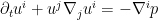
The Euler equations for incompressible inviscid fluids may be written as


where ![{u: [0,T] \times {\bf R}^n \rightarrow {\bf R}^n}](https://s0.wp.com/latex.php?latex=%7Bu%3A+%5B0%2CT%5D+%5Ctimes+%7B%5Cbf+R%7D%5En+%5Crightarrow+%7B%5Cbf+R%7D%5En%7D&bg=ffffff&fg=000000&s=0&c=20201002)
![{p: [0,T] \times {\bf R}^n \rightarrow {\bf R}}](https://s0.wp.com/latex.php?latex=%7Bp%3A+%5B0%2CT%5D+%5Ctimes+%7B%5Cbf+R%7D%5En+%5Crightarrow+%7B%5Cbf+R%7D%7D&bg=ffffff&fg=000000&s=0&c=20201002)


The Euler equations are the inviscid limit of the Navier-Stokes equations; as discussed in my previous post, one potential route to establishing finite time blowup for the latter equations when
Perhaps the most prominent obstacles to this route are the conservation laws for the Euler equations, which limit the types of final states that a putative computer could reach from a given initial state. Most famously, we have the conservation of energy

(assuming sufficient decay of the velocity field at infinity); thus for instance it would not be possible for a computer to generate a replica of itself which had greater total energy than the initial computer. This by itself is not a fatal obstruction (in this paper of mine, I constructed such a “computer” for an averaged Euler equation that still obeyed energy conservation). However, there are other conservation laws also, for instance in three dimensions one also has conservation of helicity
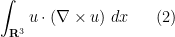
and (formally, at least) one has conservation of momentum

and angular momentum

(although, as we shall discuss below, due to the slow decay of

is also conserved, although it turns out in three dimensions that this quantity vanishes when one assumes sufficient decay at infinity. Then there are the pointwise conservation laws: the vorticity and the volume form are both transported by the fluid flow, while the velocity field (when viewed as a covector) is transported up to a gradient; among other things, this gives the transport of vortex lines as well as Kelvin’s circulation theorem, and can also be used to deduce the helicity conservation law mentioned above. In my opinion, none of these laws actually prohibits a self-replicating computer from existing within the laws of ideal fluid flow, but they do significantly complicate the task of actually designing such a computer, or of the basic “gates” that such a computer would consist of.
Below the fold I would like to record and derive all the conservation laws mentioned above, which to my knowledge essentially form the complete set of known conserved quantities for the Euler equations. The material here (although not the notation) is drawn from this text of Majda and Bertozzi.
For reasons which may become clearer later, I will rewrite the Euler equations in the language of Riemannian geometry, in particular, using the abstract index notation of Penrose), and using the Euclidean metric 


In particular we have
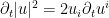
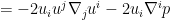
which leads to the conservation of energy (1) upon integrating in space.
In the usual treatment of the Euler equations, it is common to introduce the material derivative

Here, we shall adopt the subtly different (but closely related) approach of using the material Lie derivative

where 


However, the two notions differ when applied to vector fields or forms, with the material Lie derivative having better covariance properties than the material derivative. When applied to vector fields 
and so

Similarly, for 

and similarly for 


leading to similar formulae comparing 

Since 

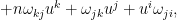
The material Lie derivative of the covelocity field 


In particular, we see that the material Lie derivative of the covelocity is a gradient:

Since the integral of a gradient along any closed loop is zero, we obtain
Theorem 1 (Kelvin’s circulation theorem) Let
be a time-dependent loop in
for any scalar function
). Then

Now we take an exterior derivative of the covelocity

In abstract index notation, 

As exterior derivatives commute with diffeomorphisms, they also commute with Lie derivatives, so in particular
Since 

(This fact was also interpreted as conservation of exterior momentum in this previous blog post.) This fact also follows from Kelvin’s circulation theorem, after first applying Stokes’ theorem to rewrite 


If we let 
If we thus define the polar vorticity 

for all 
In two dimensions 

In three dimensions 


From (7) we also see that the vortex lines are transported by the flow; in fact we have the stronger statement that if ![{\gamma: [0,T] \times {\bf R} \rightarrow {\bf R}^3}](https://s0.wp.com/latex.php?latex=%7B%5Cgamma%3A+%5B0%2CT%5D+%5Ctimes+%7B%5Cbf+R%7D+%5Crightarrow+%7B%5Cbf+R%7D%5E3%7D&bg=ffffff&fg=000000&s=0&c=20201002)

at the initial time 

In three dimensions, we may contract the polar vorticity 


Now the exterior derivative of 


Finally, we consider the conservation of various moments of the velocity and vorticity. Here it is best to return to material derivatives 
Because we will be considering linear integrals of 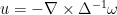

We begin with the total vorticity

which is well-defined as a 


and hence also the total vorticity. Namely, if 


and integration in parts (now involving the compactly supported vorticity 
In any dimension, though, the total vorticity (and hence also total polar vorticity) is conserved. Indeed, from (5) and (3) we have


where we have used the vanishing 


giving conservation of total vorticity.
Now we look at total velocity

which (up to a scaling factor representing the density of the incompressible fluid) has the physical interpretation as the total momentum of the fluid. We have

which formally suggests that total velocity is conserved. However, in practice


Thus, when

however, the right-hand side remains well defined even when

in three dimensions, this would be 


and so it will suffice to show that 

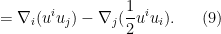
Finally, we look at the total angular momentum

Again, we have


which as before formally suggests that total angular momentum should be conserved. As with total momentum, in practice the velocity field ![{(a_{jk})_{[j,k]} := a_{jk}-a_{kj}}](https://s0.wp.com/latex.php?latex=%7B%28a_%7Bjk%7D%29_%7B%5Bj%2Ck%5D%7D+%3A%3D+a_%7Bjk%7D-a_%7Bkj%7D%7D&bg=ffffff&fg=000000&s=0&c=20201002)

![\displaystyle x^i \omega_{ij} x_k - x^i \omega_{ik} x_j = (x^i \omega_{ij} x_k)_{[j,k]}](https://s0.wp.com/latex.php?latex=%5Cdisplaystyle+x%5Ei+%5Comega_%7Bij%7D+x_k+-+x%5Ei+%5Comega_%7Bik%7D+x_j+%3D+%28x%5Ei+%5Comega_%7Bij%7D+x_k%29_%7B%5Bj%2Ck%5D%7D&bg=ffffff&fg=000000&s=0&c=20201002)
![\displaystyle = ( x^i x_k \partial_i u_j - x^i x_k \partial_j u_i )_{[j,k]}](https://s0.wp.com/latex.php?latex=%5Cdisplaystyle+%3D+%28+x%5Ei+x_k+%5Cpartial_i+u_j+-+x%5Ei+x_k+%5Cpartial_j+u_i+%29_%7B%5Bj%2Ck%5D%7D&bg=ffffff&fg=000000&s=0&c=20201002)
![\displaystyle = ( \partial_i(x^i x_k u_j) - \partial_j (x^i x_k u_i) - n x_k u_j - x^i u_i \eta_{jk} )_{[j,k]}](https://s0.wp.com/latex.php?latex=%5Cdisplaystyle+%3D+%28+%5Cpartial_i%28x%5Ei+x_k+u_j%29+-+%5Cpartial_j+%28x%5Ei+x_k+u_i%29+-+n+x_k+u_j+-+x%5Ei+u_i+%5Ceta_%7Bjk%7D+%29_%7B%5Bj%2Ck%5D%7D&bg=ffffff&fg=000000&s=0&c=20201002)
![\displaystyle = ( \partial_i(x^i x_k u_j) - \partial_j (x^i x_k u_i) )_{[j,k]} - n(u_j x_k - u_k x_j)](https://s0.wp.com/latex.php?latex=%5Cdisplaystyle+%3D+%28+%5Cpartial_i%28x%5Ei+x_k+u_j%29+-+%5Cpartial_j+%28x%5Ei+x_k+u_i%29+%29_%7B%5Bj%2Ck%5D%7D+-+n%28u_j+x_k+-+u_k+x_j%29&bg=ffffff&fg=000000&s=0&c=20201002)
and so we have

when there is sufficient decay of the velocity field. Again, the right-hand side makes sense whenever the vorticity is compactly supported. If we then define the moment of impulse
then we expect this quantity to also be conserved by the flow. This is indeed the case, and can be verified by a rather lengthy calculation similar to that used to establish conservation of impulse; we omit the details here as they are rather tedious and unenlightening, with a key step being the establishment of the fact that ![{(u^i \omega_{ij} x_k)_{[j,k]}}](https://s0.wp.com/latex.php?latex=%7B%28u%5Ei+%5Comega_%7Bij%7D+x_k%29_%7B%5Bj%2Ck%5D%7D%7D&bg=ffffff&fg=000000&s=0&c=20201002)

27 comments
Comments feed for this article
25 February, 2014 at 2:29 pm
MrCactu5 (@MonsieurCactus)
It is as if you dropped leaves on a pond… How unfortunate that energy, angular momentum and vorticity conserved here. What are the corresponding symmetries, by Noether theorem?
I have been contented with some hand-wavy definitions + illustrations. Glad to learn the Euler equations do indeed conserve twirliness, upon time evolution.
25 February, 2014 at 3:04 pm
Anonymous
Hi, I think that you may have missed embedding the link to Majda’s and Bertozzi’s text at the end of the “Below the fold…” paragraph.
[Corrected, thanks – T.]
25 February, 2014 at 3:05 pm
interested non-expert
1) “is drawn from this text of Majda and Bertozzi.” – the link is missing.
2) “I constructed such a “computer” for an averaged Euler equation” – i thought the result was for an averaged Navier-Stokes, instead of euler equation?
[The result applies to both equations (the viscosity term should be viewed as a lower order perturbative error), but in the current context, the Euler equation setting is more relevant. -T.]
25 February, 2014 at 6:16 pm
Anonymous
What suggested in Section 1.3 of that paper is actually for the Euler equations. The Euler are not the true Navier-Stokes. More baffling, the comments made in the last paragraph of S1.3 imply that a finite-time singularity would have the effect of measure-zero on NS global regularity!
25 February, 2014 at 6:35 pm
tomcircle
Reblogged this on Math Online Tom Circle.
26 February, 2014 at 3:36 am
Philip Thrift
The “fluid computer” model proposed here looks like an interesting one to pursue.
26 February, 2014 at 8:34 am
Anonymous
Euler’s equations (fluid dynamics) have no sense as the exact vector equations because gradp is not a true vector function! http://books.google.com/books?id=FC0QFlx12pwC&pg=PA15%7CDubrovin
26 February, 2014 at 6:47 pm
Terence Tao
Actually, the more precise statement is that the Euler equations become geometric (coordinate independent) if the Euclidean metric (which is called in this post) is included as part of the geometric structure of physical space. Once one has this metric, one can interpret the gradient
  as a vector (rather than a covector or
  -form) by using the raising operator associated with that metric to turn the derivative
  of the pressure
  from a covector to a vector. So the Euler equations make perfect sense in the category of Euclidean spaces (and more generally, in the category of Riemannian manifolds), but not in the coarser category of smooth manifolds.
In particular, the Euler equations are not covariant with respect to general diffeomorphisms (unless one also transforms the Euclidean metric together with all the other fields); but they are still covariant with respect to Euclidean rigid motions.
26 February, 2014 at 9:53 pm
Fan
turn the derivative of the pressure
  from a covector to a covector?
[Corrected, thanks – T.]
26 February, 2014 at 9:25 pm
Nick
Reading this reminded me a bit of the paper by Benjamin and Olver (1982, Journal of Fluid Mechanics), where the authors completely classified the conservation laws for irrotational surface water waves. This led me to a related paper by Olver that derives the conservation laws for the Euler equations through an examination of its Hamiltonian: http://www.sciencedirect.com/science/article/pii/0022247X82901007).
27 February, 2014 at 7:23 am
rapunzellindemann
Reblogged this on Anakin's reveries in multiverses.
27 February, 2014 at 8:34 am
Anonymous
This and the previous post are revolutionary works/point of views.
28 February, 2014 at 6:14 am
Navier-Stokes Fluid Computers | Combinatorics and more
[…] here is a follow up post on Tao’s […]
2 March, 2014 at 10:34 pm
Gil Kalai
A thought about the interface between the model and actual physics: Even if Euler’s equation allows for universal computation I don’t think we can expect to see memory and computation emerge in real-life fluids in nature. It is thus possible that “no memory,” “no computation” or “no fault-tolerance” represent a physical principle (perhaps of thermodynamical nature) external to the equations themselves (which accounts also for no realistic finite time blow up). This may lead also to additional conserved physical quantities which are not coming from the equation but from the equation with an added principle of “no long computation.”
And another thought: We could think about a hypothetical world in which humans are much more mathematically advanced compared to our own world, but they are less advanced in terms of other senses, other forms of understanding, and common sense. In such a world mathematical nerds may have much larger share of wealth, fame, sex, and power compared to our own world. In such a world the universal computing powers of the Euler’s equation are known to kindergarten children. It may be the case that in such a world fish would not be regarded as animals living in seas and oceans but rather as fault-tolerant fluid computers which spontaneously emerged in the oceans.
2 March, 2014 at 11:08 pm
Noether’s theorem, and the conservation laws for the Euler equations | What's new
[…] locate all of the conserved quantities for the Euler equations of inviscid fluid flow, discussed in this previous post, by interpreting that flow as geodesic flow in an infinite dimensional […]
4 March, 2014 at 10:12 pm
Gil Kalai
Dear Terry, the following question arose in a discussion over Scott Aaronson’s Shtetl-optimized in a post on the long reach of computation devoted to your paper and to a paper by Leonard Susskind. The qestion is about the “speeding up and shrinking exponentially” aspect of your work. It looks that it is required to move from universal fault-tolerance computation to finite-time blow up. But is it a crucial aspect of the universal computing part? Namely, do you expect that you will be able to simulate universal computing with computational steps being carried out in constant speed (like ordinary computers).
5 March, 2014 at 7:14 am
arch1
Aspects of this discussion remind me of Freeman Dyson’s speculation on an approach which could enable far-future intelligence in an open universe to perform an infinite amount of computation, ever more slowly, using a finite amount of energy. (I think I saw this in his 1979 book Disturbing the Universe; his 1979 paper on the topic is “”Time without end: Physics and biology in an open universe”).
(I think it was also Dyson who proposed a mechanism for an infinite amount of computation to take place ever more quickly during the ‘big crunch’ of a *closed* universe, though I don’t have a reference).
5 March, 2014 at 7:45 am
Terence Tao
My feeling (and hope) is that for performing arbitrary computations up to N steps in length, one should be able to build a universal computer that can perform those N steps with a unit time taken for each, but the size, energy, and complexity of this computer will grow quite fast with N (particularly since the “materials” one needs to build the computer out of will need to be stable for time N). Even in the absence of viscosity, I would expect entropy (and energy leakage) to eventually take over and disperse any computer after a sufficient period of time. But if one can get the computer to last for an arbitrary finite amount of time, rather than for an infinite amount of time, this should be enough to execute the finite time blowup scenario via programming the computer to build a smaller, faster replica of itself in a time less than the useful working lifetime of that computer. (But, in the absence of such programming, the computer has no particular propensity to shrink or speed up.)
6 March, 2014 at 11:33 am
Gil Kalai
Thanks! Often if you can achieve robust computation you can put on top fault-tolerance mechanism based on error-correction that will reduce entropy by discarding some undesired elements. So this may lead to implementations where the size,energy and complexity scales up modestly with N. However, it looks that this aspect is not needed for now for finite-time blow up (perhaps such blowup depends just on the ability to compute and not on the ability to carry out efficient computations efficiently.)
Another unrealated question: Beside the average model are there other cases where your program might be easier, e.g. in high dimensions?
6 March, 2014 at 12:49 pm
Terence Tao
Higher dimensions should be a little easier, because the conservation laws are less obstructive (for instance, the 3D phenomenon of vortex lines being transported by the flow, which could potentially produce some topological obstructions, is no longer present; for similar reasons, helicity conservation disappears in higher dimensions). Also the effect of viscosity is less (relative to the nonlinear effects), so one can afford to be a little less energy-efficient with regard to the self-similar blowup scenario. One could also throw out viscosity altogether and just shoot for blowup in the Euler equations, which may be a little simpler technically (in particular, all the conservation laws for the Euler equations hold exactly rather than approximately).
In the other direction, the two-dimensional surface quasi-geostrophic (SQG) equations (the topic of my most recent blog post) are a somewhat simpler toy model of the Euler equations which may be easier to analyse from a geometric or topological viewpoint, although these equations have more conservation laws and it may be more difficult to perform complex computing within this system (and in two spatial dimensions there may be additional difficulties in building objects such as valves and tubes which we are accustomed to being easily constructible in three dimensions).
Moving away from the “named equations” of fluid dynamics, one could also look at more artificial fluid-like equations which are closer to the true fluid equations than the averaged Navier-Stokes equations considered in my paper. For instance one could imagine a carefully constructed system of multiple fluids occupying the same region of physical space, and interacting with each other in a manner designed to facilitate computation: for instance one fluid could be a lot “stiffer” than another and could be used as the material for pipes, valves, etc. in which the other fluids would flow. This is sort of how my averaged equation works already, except that in my averaged equation the different fluid components occupy different regions of frequency space, rather than different regions of physical space.
6 March, 2014 at 3:08 am
Anonymous
I wonder if there should be some kind of continuum version of a symplectic form which stays invariant in the Hamiltonian flow corresponding to the NSE. This is a simple and very fundamental question, but in the few articles considering NSE in Lagrangian coordinates I have seen there has not been a mention of it.
6 March, 2014 at 8:39 am
Terence Tao
Well, firstly one would have to work with the Euler equations rather than the Navier-Stokes equations, as the latter are not time-reversible (due to the viscosity term) and thus not Hamiltonian. There is a symplectic form that is formally preserved by the Euler flow (when combined with the label map
  from Lagrangian space to Eulerian space), namely the canonical symplectic form
  on the cotangent bundle on the infinite-dimensional manifold M of volume-preserving maps from Lagrangian space to Eulerian space. In many texts though, the label map
  is dropped (analogous to ignoring (or more precisely, projecting out) a set of angle coordinates in Hamiltonian mechanics), leaving only the velocity field
  ; this causes the symplectic form to degenerate. As such, most texts using a Hamiltonian approach to the Euler equations do not deal directly with the symplectic form, but instead consider the inverse symplectic form
  , which describes the Hamiltonian vector field
  associated to a given Hamiltonian
  , or the Poisson bracket
  of two observables
  . (The degeneracy now reflects itself in the fact that some Hamiltonians will have trivial vector field in this projected dynamics, and some functions
  will be in the nullspace of the Poisson bracket.)
This paper of Olver describes the inverse symplectic form through the linear operator defining the Hamiltonian vector field for a given Hamiltonian (ignoring the label map); this paper of Vasylkevych and Marsden describes the Poisson bracket (in the full phase space that includes the label map). (I believe there is also some early work of Holm in the latter direction, but was unable to locate it.)
19 March, 2014 at 10:06 am
benedictsnow
A trivial thing to point out, I know, but should the line “[t]he material Lie derivative of the covelocity field is however more interesting
 ”
” in the last term, as opposed to
  ?
?
just after equation (3) not have an upper index
[Corrected, thanks – T.]
19 March, 2014 at 10:41 am
benedictsnow
Also noticed “Now we take an exterior derivatives” just after Theorem 1.
[Corrected, thanks – T.]
24 April, 2014 at 3:02 am
Henrik Rasmussen
Very interesting post. Just a small point: is there not a minus missing in your Biot-Savart law ? (twice curl = – laplacian on solenoidal vector fields).
[Corrected, thanks – T.]
4 June, 2014 at 6:28 am
Anonymous
Compared to real fluid flows, it is a different story for inviscid flows governed by the Euler equation. There exists a view that Euler solutions will blow up in finite time. A number of recent preprints suggest that Euler solutions show norm inflation (even in some smooth function spaces). The inflation may be considered as scenarios close to blow-ups. Unfortunately, these claims are misleading as they are based on ill-defined analyses.
26 February, 2018 at 7:24 am
harmeet1987
Looks like there is an index mismatch in your definition of the material lie derivative of vector fields. The index ‘i’ on the first term on the right side should be up (D_t X^i)I suppose.
[Corrected, thanks – T.]