We continue the discussion of sieve theory from Notes 4, but now specialise to the case of the linear sieve in which the sieve dimension  is equal to
  , which is one of the best understood sieving situations, and one of the rare cases in which the precise limits of the sieve method are known. A bit more specifically, let
  be quantities with
  for some fixed
  , and let
  be a multiplicative function with

and

for all primes  and some fixed
  (we allow all constants below to depend on
  ). Let
  , and for each prime
  , let
, let  be a set of integers, with
  for
for  . We consider finitely supported sequences
  of non-negative reals for which we have bounds of the form
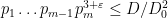
for all square-free  and some
  , and some remainder terms
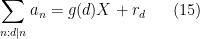
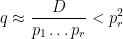
  . One is then interested in upper and lower bounds on the quantity

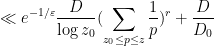
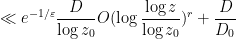
The fundamental lemma of sieve theory (Corollary 19 of Notes 4) gives us the bound

where  is the quantity

This bound is strong when  is large, but is not as useful for smaller values of . We now give a sharp bound in this regime. We introduce the functions
  by
by

and

where we adopt the convention  . Note that for each one has only finitely many non-zero summands in (6), (7). These functions are closely related to the Buchstab function
  from Exercise 28 of Supplement 4; indeed from comparing the definitions one has
for all  .
.
Exercise 1 (Alternate definition of  ) Show that
  is continuously differentiable except at
  , and
, and  is continuously differentiable except at
  where it is continuous, obeying the delay-differential equations
for  and
and

for  , with the initial conditions
for  and
and

for  . Show that these properties of determine completely.
For future reference, we record the following explicit values of :

for  , and
, and
for  .
.
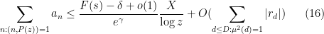
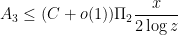
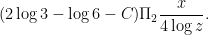
We will show
Theorem 2 (Linear sieve) Let the notation and hypotheses be as above, with . Then, for any  , one has the upper bound

and the lower bound

if  is sufficiently large depending on
  . Furthermore, this claim is sharp in the sense that the quantity cannot be replaced by any smaller quantity, and similarly cannot be replaced by any larger quantity.
Comparing the linear sieve with the fundamental lemma (and also testing using the sequence  for some extremely large
  ), we conclude that we necessarily have the asymptotics

for all  ; this can also be proven directly from the definitions of , or from Exercise 1, but is somewhat challenging to do so; see e.g. Chapter 11 of Friedlander-Iwaniec for details.
Exercise 3 Establish the integral identities

and

for  . Argue heuristically that these identities are consistent with the bounds in Theorem 2 and the Buchstab identity (Equation (16) from Notes 4).
Exercise 4 Use the Selberg sieve (Theorem 30 from Notes 4) to obtain a slightly weaker version of (12) in the range  in which the error term
  is worsened to
  , but the main term is unchanged.
We will prove Theorem 2 below the fold. The optimality of is closely related to the parity problem obstruction discussed in Section 5 of Notes 4; a naive application of the parity arguments there only give the weak bounds  and
and  for , but this can be sharpened by a more careful counting of various sums involving the Liouville function
  .
.
As an application of the linear sieve (specialised to the ranges in (10), (11)), we will establish a famous theorem of Chen, giving (in some sense) the closest approach to the twin prime conjecture that one can hope to achieve by sieve-theoretic methods:
Theorem 5 (Chen’s theorem) There are infinitely many primes such that  is the product of at most two primes.
The same argument gives the version of Chen’s theorem for the even Goldbach conjecture, namely that for all sufficiently large even , there exists a prime between  and such that
  is the product of at most two primes.
The discussion in these notes loosely follows that of Friedlander-Iwaniec (who study sieving problems in more general dimension than  ).
).
— 1. Optimality —
We first establish that the quantities  appearing in Theorem 2 cannot be improved. We use the parity argument of Selberg, based on weight sequences
  related to the Liouville function.
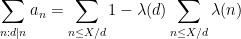
We argue for the optimality of ; the argument for is similar and is left as an exercise. Suppose that there is for which the claim in Theorem 2 is not optimal, thus there exists  such that

for  as in that theorem, with
  sufficiently large.
We will contradict this claim by specialising to a special case. Let be a large parameter going to infinity, and set  . We set
  , then by Mertens’ theorem we have
  . We set to be the residue class
  , thus (3) becomes
and (14) becomes
where .
Now let be a small fixed quantity to be chosen later, set  , and let be the sequence
This is clearly finitely supported and non-negative. For any  , we have
from the multiplicativity of . If , then  , and then by the prime number theorem for the Liouville function (Exercise 41 from Notes 2, combined with Exercise 18 from Supplement 4) we have

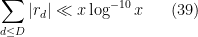
(say), annd hence the remainder term in (15) is of size

As such, the error term  in (16) may be absorbed into the
  term, and so
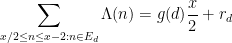
Now we count the left-hand side. Observe that  is supported on those numbers
  that are the product of an odd number of primes
  (possibly with repetition), in which case
  . To be coprime to
  , all these primes must be at least ; since we are restricting
  , we thus must have
  . The left-hand side of (18) may thus be written as

This expression may be computed using the prime number theorem:
Exercise 6 Show that the expression (19) is equal to  .
.
Since  is continuous for , we obtain a contradiction if
  is sufficiently small.
Exercise 7 Verify the optimality of in Theorem 2. (Hint: replace by  in the above arguments.)
— 2. The linear sieve —
We now prove the forward direction of Theorem 2. Again, we focus on the upper bound (12), as the lower bound case is similar.
Fix . Morally speaking, the most natural sieve to use here is the (upper bound) beta sieve from Notes 4, with the optimal value of  , which for the linear sieve turns out to be
  . Recall that this sieve is defined as the sum

where  is the set of divisors
  of with
  , such that

for all odd  . From Proposition 14 of Notes 4 this is indeed an upper bound sieve; indeed we have

where  is the set of divisors
  of with
  , such that
and

for all odd  . Now for the key heuristic point: if
  lies in the support of
  , then the sum in (20) mostly vanishes. Indeed, if
  is such that
  and
and  for some
  and odd
  , then one has
  for some
  that is not divisible by any prime less than
  . On the other hand, from (21), (22) one has
and

which (morally) implies from the sieve of Erathosthenes that is prime, thus  and so
  is not in the support of . As such, we expect the upper bound sieve
 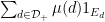 to be extremely efficient on the support of , which when combined with the analysis of the previous section suggests that this sieve should produce the desired upper bound (12).
One can indeed use this sieve to establish the required bound (12); see Chapter 11 of Friedlander-Iwaniec for details. However, for various technical reasons it will be convenient to modify this sieve slightly, by increasing the parameter to be slightly greater than , and also by using the fundamental lemma to perform a preliminary sifting on the small primes.
We turn to the details. To prove (12) we may of course assume that  is suitably small. It will be convenient to worsen the error
  in (12) a little to
  , since one can of course remove the logarithm by reducing appropriately.
Set  and
and  . By the fundamental lemma of sieve theory (Lemma 17 of Notes 4), one can find combinatorial upper and lower bound sieve coefficients
  at sifting level
  supported on divisors of
  , such that

Thus we have  and
and

for all .
We will use the upper bound sieve  as a preliminary sieve to remove the for
  ; the lower bound sieve
  plays only a minor supporting role, mainly to control the difference between the upper bound sieve
  .
.
Next, we set  , and let
  be the upper bound beta sieve with parameter
  on the primes dividing
  up to level of distribution
  . In other words, consists of those divisors of with
  such that
for all odd  ; in particular,
  for all
  . By Proposition 14 of Notes 4, this is indeed an upper bound sieve for the primes dividing :
Multiplying this with the second inequality in (24) (this is the method of composition of sieves), we obtain an upper bound sieve for the primes up to :
Multiplying this by and summing in , we conclude that

Note that each product  appears at most once in the above sum, and all such products are squarefree and at most . Applying (3), we thus have

Thus to prove (12), it suffices to show that
for sufficiently large depending on . Factoring out the  summation using (23), it thus suffices to show that

Now we eliminate the role of . From (1), (5) and Mertens’ theorem we have

for large enough. Also, if , then and all prime factors of are at least  . Thus has at most
  prime factors, each of which are at least . From (1) we then have
The contribution of the error term  is then easily seen to be
  for large enough, and so we reduce to showing that
One can proceed here by evaluating the left-hand side directly. However, we will proceed instead by using the weight function from the previous section. More precisely, we will evaluate the expression

in two different ways, where  is as before (but with the role of
  now replaced by the function
  ). Firstly, since
  , we see from the argument used to establish (17) that
(say). Since each appears at least once, we can thus write (26) as

which upon factoring the sum using (23) and Mertens’ theorem

Thus to verify (25), it will suffice to show that (26) is of the form
for sufficiently large.
To do this, we abbreviate (26) as

where  are the sieves

By Proposition 14 of Notes 4, we can expand  as
as

where for any  , is the collection of all divisors of with
  such that

but

for all with the same parity as . For technical reasons, we will also impose the additional inequality

for all with the opposite parity as ; this follows from (30) when  , but is an additional constraint when
  and is even, but in the above identity is odd, so this additional constraint is harmless. For similar reasons we impose the inequality

which follows from (30) or (31) except when  , but then this inequality is automatic from our hypothesis , which implies
  if is chosen small enough.
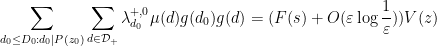
Inserting the identity (28), we can write (26) as

where
and
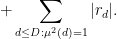
We first estimate  . By(24), we can write as the sum of
plus an error of size at most

(where we bound  by
by  ). The error may be rearranged as

which by (23) is of size  for small enough. As for the main term (33), we see from Exercise 6 (and the arguments preceding that exercise) that this term is equal to
  for sufficiently large. Thus, to obtain the desired approximation for (26), it will suffice to show that
Next, we establish an exponential decay estimate on the  :
:
Lemma 8 For sufficiently large depending on , we have

for all and some absolute constant  .
.
Proof: (Sketch) Note that if is in , then and all prime factors are at least  , thus we may assume without loss of generality that
  .
.
We bound

Note that if lies in , then

thanks to (29), (32). From this and the fundamental lemma of sieve theory we see (Exercise!) that

and so it will suffice to show that

By the prime number theorem, the left-hand side is bounded (Exercise!) by  as
as  , where
and 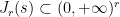 is the set of points
  with
with  ,
,

and such that

for all with the same parity as , and

for all  . It thus suffices to prove the bound

for all and some absolute constant  .
.
We use an argument from the book of Harman. Observe that  vanishes for
  , which makes the claim (35) routine for (Exercise!) for
  sufficiently large. We will now inductively prove (35) for all odd . From the change of variables
  , we obtain the identity

where  when is odd and
  when is even (Exercise!). In particular, if
  is odd and (35) was already proven for
  , then


One can check (Exercise!) that the quantity  is maximised at
  , where its value is less than (in fact it is
  ) if is small enough. As such, we obtain (35) if
  is sufficiently close to .
Finally, (35) for even follows from the odd case (with a slightly larger choice of ) by one final application of (36). 
Exercise 9 Fill in the steps marked (Exercise!) in the above proof.
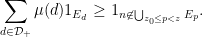
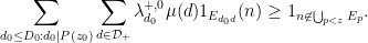
In view of this lemma, the total contribution of with  for some sufficiently large is acceptable. Thus it suffices to show that

whenever  is odd.
By (24), we can write as
plus an error of size

Arguing as in the treatment of the term, we see from (23) that the error term is bounded by


as desired for large enough, since  and
and  . Thus it suffices to show that

If and appear in the above sum, then we have where  has no prime factor less than , has an even number of prime factors, and obeys the bounds

thanks to (29). Note that (29) also gives  , and thus (since
  and
and  ) we see that
  if is small enough and is large enough. This forces to either equal , or be the product of two primes between and
  . The contribution of the
  case is bounded by
  , which is acceptable. As for the contribution of those that are the product of two primes, the prime number theorem shows that there are at most

values of that can contribute to the sum, and so this contribution to is at most

but by (34) the sum here is for large enough, and the claim follows. This completes the proof of (12).
Exercise 10 Establish the lower bound (13) in Theorem 2. (Note that one can assume without loss of generality that , which will now be needed to ensure (31) when .)
— 3. Chen’s theorem —
We now prove Chen’s theorem for twin primes, loosely following the treatment in Chapter 25 of Friedlander-Iwaniec. We will in fact show the slightly stronger statement that

for sufficiently large  , where
  is the set of all numbers that are products of at most two primes, and
  . Indeed, after removing the (negligible) contribution of those that are powers of primes, this estimate would imply that there are infinitely many primes such that is the product of at most two primes, each of which is at least
  .
.
Chen’s argument begins with the following simple lower bound sieve for  :
:
Lemma 11 If  , then
Proof: If has no prime factors less than or equal to  , then
  and the claim follows. If has two or more factors less than or equal to , then
 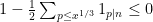 and the claim follows. Finally, if has exactly one factor less than or equal to , then (as
  ) it must be of the form
  for some
  , or it is divisible by
  for some
  , and the claim again follows.
In view of this sieve (trivially managing the contribution of  or of the case where
  , and using the restriction of
  to be coprime to ), it suffices to show that
for sufficiently large , where
and

We thus seek sufficiently good lower bounds on  and sufficiently good upper bounds on
  and
and  . As it turns out, the linear sieve, combined with the Bombieri-Vinogradov theorem, will give bounds on
  with numerical constants that are sufficient for this purpose.
We begin with . We use the lower bound linear sieve, with equal to the residue class  for all , so that
  is the residue class
  . We approximate
where is the multiplicative function with  and
and  for
for  . From the Bombieri-Vinogradov theorem (Theorem 17 of Notes 3) we have
(say) if  for some small fixed . Applying the lower bound linear sieve (13), we conclude that

where

We can compute an asymptotic for  :
:
Exercise 12 Show that

as , where  is the twin prime constant.
From (11) we have  . Sending slowly to zero, we conclude that

Now we turn to . Here we use the upper bound linear sieve. Let be as before. For any dividing and  , we have

where and are as previously. We apply the upper bound linear sieve (12) with level of distribution  , to conclude that

We sum over . Since  is at most , and each number less than or equal to has at most
  prime factors, we have


The error term is  thanks to (39). Since
  , we thus have

for sufficiently large , thanks to Exercise 12. We can compute the sum using Exercise 37 of Notes 1, to obtain

which by (10) and sending  slowly gives

A routine computation shows that
and so

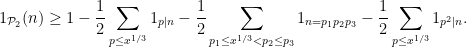
Finally, we consider , which is estimated by “switching” the sieve to sift out small divisors of , rather than small divisors of . Removing those with  , as well as those that are powers of primes, and then shifting by , we have

where is the finitely supported non-negative sequence
Here we are sifting out the residue classes  , so that
  .
.
The sequence has good distribution up to level :
Proposition 13 One has

where is as before, and

(say), with as before.
Proof: Observe that the quantity  in (42) is bounded above by
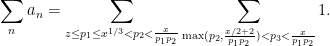
  if the summand is to be non-zero. We now use a finer-than-dyadic decomposition trick similar to that used in the proof of the Bombieri-Vinogradov theorem in Notes 3 to approximate as a combination of Dirichlet convolutions. Namely, we set
  , and partition
 ![{[x^{1/3},x^{2/3}]}](https://s0.wp.com/latex.php?latex=%7B%5Bx%5E%7B1%2F3%7D%2Cx%5E%7B2%2F3%7D%5D%7D&bg=ffffff&fg=000000&s=0&c=20201002) (plus possibly a little portion to the right of ) into
(plus possibly a little portion to the right of ) into  consecutive intervals
  each of the form
 ![{[N, \lambda N]}](https://s0.wp.com/latex.php?latex=%7B%5BN%2C+%5Clambda+N%5D%7D&bg=ffffff&fg=000000&s=0&c=20201002) for some
for some  . We similarly split
 ![{[z,x^{1/3}]}](https://s0.wp.com/latex.php?latex=%7B%5Bz%2Cx%5E%7B1%2F3%7D%5D%7D&bg=ffffff&fg=000000&s=0&c=20201002) (plus possibly a tiny portion of
(plus possibly a tiny portion of ![{[z/2,z]}](https://s0.wp.com/latex.php?latex=%7B%5Bz%2F2%2Cz%5D%7D&bg=ffffff&fg=000000&s=0&c=20201002) ) into
) into  intervals
  each of the form
 ![{[M, \lambda M]}](https://s0.wp.com/latex.php?latex=%7B%5BM%2C+%5Clambda+M%5D%7D&bg=ffffff&fg=000000&s=0&c=20201002) for some
for some  . We can thus split as

Observe that for each  there are only choices of
  for which the summand can be non-zero. As such, the contribution of the diagonal case
  can be easily seen to be absorbed into the error, as can those cases where the product set
  is not contained completely in
 ![{[x/2+2,x]}](https://s0.wp.com/latex.php?latex=%7B%5Bx%2F2%2B2%2Cx%5D%7D&bg=ffffff&fg=000000&s=0&c=20201002) . If we let
. If we let  be the set of triplets
  obeying these properties, we can thus approximate by
  , where
  is the Dirichlet convolution

From the general Bombieri-Vinogradov theorem (Theorem 16 of Notes 3) and the Siegel-Walfisz theorem (Exercise 64 of Notes 2) we see that

where

(say) and

This gives the claim with  replaced by the quantity
  ; but by undoing the previous decomposition we see that this quantity is equal to up to an error of
  (say), and the claim follows.
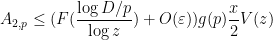
Applying the upper bound sieve (12) (with sifting level  ), we thus have

and hence by (10) and Exercise 12

for sufficiently large.
Note that
From the prime number theorem and Exercise 37 of Notes 1, we thus have

(In fact one also has a matching lower bound, but we will not need it here.) We thus conclude that
where


The left-hand side of (38) is then at least
One can calculate that  , and the claim follows.
Exercise 14 Establish Chen’s theorem for the even Goldbach conjecture.
Remark 15 If one is willing to use stronger distributional claims on the primes than is provided by the Bombieri-Vinogradov theorem, then one can use a simpler sieve than Chen’s sieve to establish Chen’s theorem, but then the required distributional theorem will then either be conjectural or more difficult to establish than the Bombieri-Vinogradov theorem. See Chapter 25 of Friedlander-Iwaniec for further discussion.


23 comments
Comments feed for this article
29 January, 2015 at 4:16 pm
Eytan Paldi
It seems that in the RHS of (6)-(7), “ ” (in the integrands) should be “
 “.
“.
[Corrected, thanks – T.]
29 January, 2015 at 5:32 pm
Eytan Paldi
Also in the line below (7).
[Corrected, thanks – T.]
29 January, 2015 at 7:41 pm
arch1
In the last two integrals preceding Exercise 9, the upper integration limit is misplaced.
[Corrected, thanks -T.]
29 January, 2015 at 7:50 pm
arch1
3 lines up from (37): we see from (23) *that the error*(?) is bounded by
[Corrected, thanks -T.]
1 February, 2015 at 8:46 am
Lior Silberman
In the proof of Chen’s Theorem, in the paragraph “We begin with “,
“,  is said to be the class of -2 mod
  rather than mod
  .
.
[Corrected, thanks – T.]
31 March, 2015 at 7:58 am
Karaskas
Just after the fragment “and the Siegel-Walfisz theorem (Exercise 64 of Notes 2) we see that [Formula] where” it should probably be log^{-10}x instead of log^{-100x}.
[Corrected, thanks – T.]
31 March, 2015 at 1:20 pm
Karaskas
Right now it’s log^{-10x} instead of log^{-10}x.
[Corrected, thanks – T.]
10 April, 2015 at 3:07 pm
Karaskas
Chen’s theorem section: shouldn’t it be under the big sigma in the definition of
  ? The same thing reappears a few lines later.
Just after “Now we turn to “, what happens if p divides d?
[I was not able to locate this issue – T.]
11 April, 2015 at 12:43 am
Karaskas
In the same fragment it probably should be instead of
  , shouldn’t it? That would also explain my last question.
[Corrected, thanks – T.]
11 April, 2015 at 9:53 am
Karaskas
The issue wasn’t there anymore while I was writting about it. I think you had repaired it a few days before and I forgot to refresh the website. Sorry for the confusion.
By the way, thank you for writing posts about sieve theory. Some details and ideas are much easier for me to follow right now.
14 April, 2015 at 2:49 pm
Karaskas
The formula under “Applying the upper bound sieve” fragment: it should be instead of
  in one place.
[Corrected, thanks – T.]
15 December, 2015 at 5:04 pm
Karaskas
I have a little confusion: before the equation (40) we send {\varepsilon} to 0 slowly but in Theorem 2 we have “if {D} is sufficiently large depending on {\varepsilon, s, c}.” How should I understand this?
15 December, 2015 at 6:23 pm
Karaskas
It seems to me like we are using two different epsilons there. By the way, is it possible to relax conditions in Theorem 2 and let depend on z?
Theorem 2 also reminds me the Jurkat-Richert theorem, although we do not have any restriction on the sieve dimension. How do these two theorems are related to each other?
Sorry for doubling the post and using LaTeX wrongly in the previous one.
15 December, 2015 at 7:13 pm
Terence Tao
For any fixed choice of , the largeness condition on
  required for Theorem 2 will apply if
  is large enough, thus
whenever is sufficiently large depending on
  (this allows for the o(1) errors to be absorbed into the
  error). In particular, for any
  , one has
whenever is sufficiently large depending on
  (by choosing
  appropriately depending on
  ). This implies that
as .
.
Another way to think about it as follows: if one has a bound of the form
as for any fixed choice of
  , then one automatically has the improvement
as , by setting
  equal to a function of
  that goes to zero sufficiently slowly (slow enough so that the
  error in (1) still goes to zero even though
  is now varying).
The Jurkat-Richert theorem has a slightly better error term replacing , and a slightly worse error term for the
  errors, but can easily be used as a substitute for Theorem 2 for the purpose of proving Chen’s theorem.
30 December, 2015 at 6:32 pm
Karaskas
I have one problem with Lemma 11. How do we rule out the numbers of the form , where
  and
and  and
and  ?
?
I saw an another proof of Chen’s theorem in which the author (Nathanson, I guess) used the sum instead of
  . By this trick we can easily avoid thinking about numbers which are not square-free.
Are these two approaches equivalent in some easy way which I cannot see right now?
I would also like to thank you for your last answer.
[Oops, this case does need to be inserted, but it is easily dealt with (with , it contributes
  from trivial estimates). -T.]
10 July, 2019 at 2:51 pm
Anonymous
Why is of in Chen’s Theorem? Is it not the case that the closer
  is to
is to  the better? I believe that using the same arguments and with same error term, one could set
  , where
  is the root of
  , i.e,
  .
.
10 July, 2019 at 5:04 pm
Terence Tao
In this post I am not attempting to optimise the exponents in order to keep the exposition as clean as possible. I believe the text of Friedlander-Iwaniec contains further improvements to the exponent for , but I do not have the reference handy right now, and there may be further slight improvements in the literature.
UPDATE: Section 25.6 of Friedlander-Iwaniec allows to be as large as
  . It may be that further improvements are still possible beyond this exponent.
25 February, 2020 at 4:54 pm
Anonymous
Hi Prof Tao,
Just a quick question: why do we need eq. (31)? We seem to never use it in the proof. Apologies if I missed a clear usage of it.
26 February, 2020 at 4:43 pm
Terence Tao
(31) is needed to establish some cases of (32), which is then used in the proof of Lemma 8. (One could cut out the middle man and just impose (32), but this formalism is closer to the general beta-sieve formalism one sees for instance in the text of Iwaniec-Kowalski or Friedlander-Iwaniec.)
23 March, 2020 at 7:11 am
Michelangelo Mecozzi
A tiny detail: when we define and
and  should the values be swapped? With the current values we have
  and I assume we want
  as in the proof.
23 March, 2020 at 7:28 am
Michelangelo Mecozzi
My bad, actually we want that and it wouldn’t make sense to swap! I was working on the Exercise trying to show that the LHS of (34) is bounded by , this should be be
  or I’m mistaken again? Doesn’t make any difference in the calculations…
[Corrected, thanks – T.]
26 March, 2020 at 4:44 pm
Anonymous
Is it possible to get the following clarification: when you say (towards the end of the proof of the linear sieve) “Note that (29) also gives ” how can we deduce that?
[You are right, this is not the correct way to get a lower bound on at this step. I will have to look at Friedlander-Iwaniec for the correct argument, but unfortunately due to the lockdown I will not be able to do so for a while. -T]
5 April, 2020 at 7:53 am
Terence Tao
I was finally able to retrieve my copy of Friedlander-Iwaniec. Theorem 2 is proven (in a stronger and more general form) as Theorem 11.12 from that paper. However the arguments are quite intricate, in particular the upper bounds on are proven recursively. I now vaguely remember finding an alternate approach (based on using the Selberg counterexample weights) to write the notes here, but as you pointed out the lower bounding of
  is incorrect. If one does compute what (29), (30) do give for lower bounds, they are more of the form
  , thus the exponent degrades exponentially in
  rather than linearly. This still gives satisfactory control on the
  when
when  but now there is an intermediate region
  which is not currently covered by the above arguments. The issue is probably fixable, for instance by importing some of the recursive arguments from Friedlander-Iwaniec, but currently I will not have the time to address them and for now one should simply refer to Theorem 11.12 of Friedlander-Iwaniec for a proof of Theorem 2 in this post.