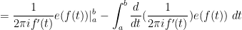
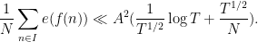
We return to the study of the Riemann zeta function  , focusing now on the task of upper bounding the size of this function within the critical strip; as seen in Exercise 43 of Notes 2, such upper bounds can lead to zero-free regions for
  , which in turn lead to improved estimates for the error term in the prime number theorem.
In equation (21) of Notes 2 we obtained the somewhat crude estimates

for any  and
and  with
with  and
and  . Setting
  , we obtained the crude estimate
in this region. In particular, if  and
and  then we had
  . Using the functional equation and the Hadamard three lines lemma, we can improve this to
  ; see Supplement 3.
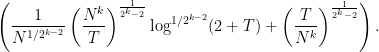
Now we seek better upper bounds on . We will reduce the problem to that of bounding certain exponential sums, in the spirit of Exercise 34 of Supplement 3:
Proposition 1 Let with and . Then

where  .
.
Proof: We fix a smooth function  with
with  for
for  and
and  for
for  , and allow implied constants to depend on
  . Let
. Let  with
with  . From Exercise 34 of Supplement 3, we have
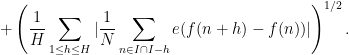
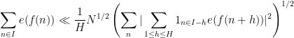
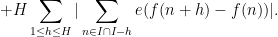
for some sufficiently large absolute constant  . By dyadic decomposition, we thus have

We can absorb the first term in the second using the  case of the supremum. Writing
  , where

it thus suffices to show that

for each  . But from the fundamental theorem of calculus, the left-hand side can be written as

and the claim then follows from the triangle inequality and a routine calculation. 
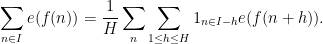
We are thus interested in getting good bounds on the sum  . More generally, we consider normalised exponential sums of the form
where  is an interval of length at most for some
  , and
, and  is a smooth function. We will assume smoothness estimates of the form
for some  , all
, all  , and all
  , where
  is the
  -fold derivative of
  ; in the case
  ,
, ![{I \subset [N,2N]}](https://s0.wp.com/latex.php?latex=%7BI+%5Csubset+%5BN%2C2N%5D%7D&bg=ffffff&fg=000000&s=0&c=20201002) of interest for the Riemann zeta function, we easily verify that these estimates hold with
of interest for the Riemann zeta function, we easily verify that these estimates hold with  . (One can consider exponential sums under more general hypotheses than (3), but the hypotheses here are adequate for our needs.) We do not bound the zeroth derivative
  of directly, but it would not be natural to do so in any event, since the magnitude of the sum (2) is unaffected if one adds an arbitrary constant to
  .
.
The trivial bound for (2) is
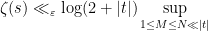
and we will seek to obtain significant improvements to this bound. Pseudorandomness heuristics predict a bound of  for (2) for any
  if
if  ; this assertion (a special case of the exponent pair hypothesis) would have many consequences (for instance, inserting it into Proposition 1 soon yields the Lindelöf hypothesis), but is unfortunately quite far from resolution with known methods. However, we can obtain weaker gains of the form
  when
when  and
and  depends on
  . We present two such results here, which perform well for small and large values of respectively:
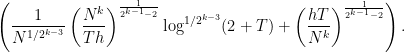
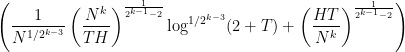
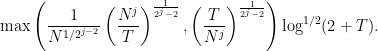
Theorem 2 Let  , let
, let  be an interval of length at most , and let
  be a smooth function obeying (3) for all and .
The factor of  can be removed by a more careful argument, but we will not need to do so here as we are willing to lose powers of
  . The estimate (6) is superior to (5) when
  for large, since (after optimising in
  ) (5) gives a gain of the form
  over the trivial bound, while (6) gives
  . We have not attempted to obtain completely optimal estimates here, settling for a relatively simple presentation that still gives good bounds on , and there are a wide variety of additional exponential sum estimates beyond the ones given here; see Chapter 8 of Iwaniec-Kowalski, or Chapters 3-4 of Montgomery, for further discussion.
We now briefly discuss the strategies of proof of Theorem 2. Both parts of the theorem proceed by treating like a polynomial of degree roughly ; in the case of (ii), this is done explicitly via Taylor expansion, whereas for (i) it is only at the level of analogy. Both parts of the theorem then try to “linearise” the phase to make it a linear function of the summands (actually in part (ii), it is necessary to introduce an additional variable and make the phase a bilinear function of the summands). The van der Corput estimate achieves this linearisation by squaring the exponential sum about times, which is why the gain is only exponentially small in . The Vinogradov estimate achieves linearisation by raising the exponential sum to a significantly smaller power – on the order of  – by using Hölder’s inequality in combination with the fact that the discrete curve
  becomes roughly equidistributed in the box
  after taking the sumset of about copies of this curve. This latter fact has a precise formulation, known as the Vinogradov mean value theorem, and its proof is the most difficult part of the argument, relying on using a “
 -adic” version of this equidistribution to reduce the claim at a given scale
  to a smaller scale
  with
with  , and then proceeding by induction.
One can combine Theorem 2 with Proposition 1 to obtain various bounds on the Riemann zeta function:
Exercise 3 (Subconvexity bound)
- (i) Show that
 for all
  . (Hint: use the
  case of the Van der Corput estimate.)
- (ii) For any
 , show that
  as
as  (the decay rate in the
  is allowed to depend on
  ).
).
Exercise 4 Let  be such that
  , and let
  .
.
- (i) (Littlewood bound) Use the van der Corput estimate to show that
 whenever
  .
.
- (ii) (Vinogradov-Korobov bound) Use the Vinogradov estimate to show that whenever
 .
.
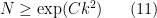
As noted in Exercise 43 of Notes 2, the Vinogradov-Korobov bound leads to the zero-free region  , which in turn leads to the prime number theorem with error term
for  . If one uses the weaker Littlewood bound instead, one obtains the narrower zero-free region
(which is only slightly wider than the classical zero-free region) and an error term

in the prime number theorem.
Exercise 5 (Vinogradov-Korobov in arithmetic progressions) Let  be a non-principal character of modulus
  .
.
— 1. Van der Corput estimates —
In this section we prove Theorem 2(i). To motivate the arguments, we will use an analogy between the sums  and the integrals
  (cf. Exercise 11 from Notes 1). This analogy can be made rigorous by the Poisson summation formula (after applying some smoothing to the integral over to truncate the frequency summation), but we will not need to do so here.
Write ![{I = [a,b]}](https://s0.wp.com/latex.php?latex=%7BI+%3D+%5Ba%2Cb%5D%7D&bg=ffffff&fg=000000&s=0&c=20201002) . We can control the integral
. We can control the integral  by integration by parts:

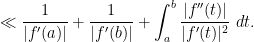
If obeys (3) for  , we thus have

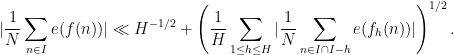
An analogous argument, using summation by parts instead of integration by parts, controls the sum  , but only in the regime when
  :
:
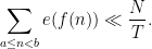
Proposition 6 Let  and , let be an interval of length at most , and let be a smooth function obeying the bounds
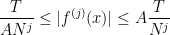
for and . If  , then

Proof: We may assume that for some integers  , and after deleting the right endpoint it suffices to show that
From the  case of (3) and the mean value theorem one has
  for all
  . Thus we have

and we can write
![\displaystyle \sum_{a \leq n < b} e(f(n)) = \sum_{a \leq n < b} [e(f(n+1)) - e(f(n))] \frac{1}{e(f(n+1)-f(n))-1}.](https://s0.wp.com/latex.php?latex=%5Cdisplaystyle+%5Csum_%7Ba+%5Cleq+n+%3C+b%7D+e%28f%28n%29%29+%3D+%5Csum_%7Ba+%5Cleq+n+%3C+b%7D+%5Be%28f%28n%2B1%29%29+-+e%28f%28n%29%29%5D+%5Cfrac%7B1%7D%7Be%28f%28n%2B1%29-f%28n%29%29-1%7D.&bg=ffffff&fg=000000&s=0&c=20201002)
From the cases of (3) and the mean value theorem we see that  has size
  and derivative
  on
on ![{[a,b-1]}](https://s0.wp.com/latex.php?latex=%7B%5Ba%2Cb-1%5D%7D&bg=ffffff&fg=000000&s=0&c=20201002) . The claim then follows from a summation by parts.
. The claim then follows from a summation by parts.
To use this proposition in the regime  , we will use the following inequality of van der Corput, which is a basic application of the Cauchy-Schwarz inequality:
Proposition 7 (van der Corput inequality) Let  , let be an interval of length , and let be a function. Then

The point of this proposition is that it effectively replaces the phase by the differenced phase  for some medium-sized
  ; it is an oscillatory version of the trivial observation that if is close to constant, then
  is also close to constant. From the fundamental theorem of calculus, we see that if obeys the estimates (3), then obeys a variant of (3) in which
  has been replaced by
  . Since
  , this reduces , and so one can hope to then iterate this proposition to the point where one can apply Proposition 6.
Proof: By rounding down, we may assume that  is an integer. For any
  , we have

and thus on averaging in
There are only  values of
  for which the inner sum is non-vanishing. By the Cauchy-Schwarz inequality, we thus have
and so it will suffice to show that

The left-hand side may be expanded as

The contribution of the diagonal terms  is
is  which is acceptable. For the off-diagonal terms, we may use symmetry to restrict to the case
  , picking up a factor of
  . After shifting by
  , we may thus bound this contribution by

Since each occurs  times as a difference
  , the claim follows.
Exercise 8 (Qualitative Weyl exponential sum estimates) Let  be a polynomial with real coefficients
  .
.
- (i) If
 and
and  is irrational, show that
  as
as  . (Hint: induct on , using geometric series for the base case
  and Proposition 7 for the induction step.)
- (ii) If and at least one of
 is irrational, show that as .
- (iii) If all of the are rational, show that
 converges as to a limit that is not necessarily zero.
One can obtain more quantitative estimates on the decay rate of in terms of how badly approximable by rationals one or more of the coefficients  are; see for instance Chapter 8 of Iwaniec-Kowalski for some estimates of this type.
If we combine one application of Proposition 7 with Proposition 6, we conclude
Proposition 9 Let and , let be an interval of length at most , and let be a smooth function obeying the bounds
for  and . Then
Proof: If then the claim follows from Proposition 6 (or from (4), if  ), so we may assume that
  . We can also assume that
  , since otherwise the claim follows from the trivial bound (4).
Set  , then
  . By Proposition 7 we have

where  . From the fundamental theorem of calculus we have

for . By Proposition 6 we then have

so on summing in

and the claim follows from the choice of .
We can iterate this:
Proposition 10 Let  be a sufficiently large constant. Then for any , any , any natural number
  , any interval of length at most , and any smooth obeying the bounds

for  and , one has

We have avoided the use of asymptotic notation for this proposition because we need to use induction on .
Proof: We induct on . The  case follows from Proposition 9. Now suppose that
  and the claim has already been proven for
  .
.
If  then the claim follows from (4) (for large enough), so suppose that
  . Then the quantity
  is such that . By Proposition 7 we have
From the fundamental theorem of calculus, obeys the bounds (7) for  with replaced by
  . Thus by the induction hypothesis,
Performing the sum over , we obtain
which by the choice of simplifies to


and the claim follows for large enough.
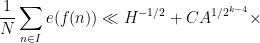
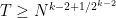
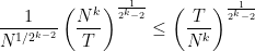
Now we can prove part (i) of Theorem 2. We can assume that , since the claim follows from (4) otherwise. For any natural number  , we can apply Proposition 10 with
  and conclude that
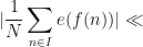
Taking infima over  , it then suffices to show that

whenever  . (The case when
  can be easily derived from the
  case, after conceding a multiplicative factor of
  .)
.)
We prove (8) by induction on . The case is clear, so suppose  and that (8) has already been proven for . If
then
and the claim follows from the  term of the infimum. If instead

then

and the claim follows from the induction hypothesis.
— 2. Vinogradov estimate —
We now prove Theorem 2(ii), loosely following the treatment in Iwaniec and Kowalski. We first observe that for bounded values of , part (ii) of this theorem follows from the already proven part (i) (replacing by, say,  ), so we may assume now that is larger than any specified absolute constant.
The first step of Vinogradov’s argument is to use a Taylor expansion and a bilinear averaging to reduce the problem to a bilinear exponential sum estimate involving polynomials with medium-sized coefficients. More precisely, we will derive Theorem 2(ii) from
Theorem 11 (Bilinear estimate) Let  be a constant, let be a sufficiently large natural number, let
  , and let be real numbers, with the property that

for at least  values of . Then

for some  depending only on
  .
.
Let us see how Theorem 2(ii) follows from Theorem 11. By reducing as necessary, we may assume that

We may also assume that
for some large constant , as the claim is trivial otherwise.
Set  . For any
  , we have

and hence on averaging in 

The condition  can only be satisfied if lies within
  of , and if lies in and is further than
  from the endpoints of then the
  constraint may be dropped. It thus suffices to show that

for all in that are further than from the endpoints of .
Fix . From (3) and Taylor expansion we see that
where  . Since
  and , we see from (11) that the error term is
  (say) if is large enough, so
and it thus suffices to show that
From (3) we have
which (since  and is large) implies from (11) that

if  (say). The claim now follows from Theorem 11 (with replaced by
  ).
).
It remains to prove Theorem 11. We fix and allow all implied constants to depend on . We may assume that

for some large constant (depending on ), as the claim is trivial otherwise.
We write the left-hand side of (10) as
where  is the bilinear form

and  is the polynomial curve
The discrete curve

lies in the box  , but occupies only a very sparse subset of this box. However, if one takes iterated sumsets

of this curve, one expects (if  is large compared with ) to fill out a much denser subset of this box (or more precisely, of a slightly larger box in which all sides have been multiplied by ), due to the “curvature” of (13). By using the device of Hölder’s inequality, we will be able to estimate the sparse sum
  with a sum over such a sumset in a box, which will be significantly easier to estimate, provided one can establish the expected density property of the sumset, or at least something reasonably close to that density property. This latter claim will be accomplished by a deep result known as the Vinogradov mean value theorem.
We turn to the details. Let be a large natural number (depending on ) to be chosen later; in fact we will eventually take  for a large absolute constant
  . From Hölder’s inequality we have

We remove the absolute values to write this as
for some coefficients  of magnitude
  . The right-hand side can be rearranged using the bilinearity of
  as
as
We collect some terms to obtain the inequality

where for each  ,
,  is the number of representations of
  of the form
  with
with  . Note that
  is supported in the box

We now use Hölder’s inequality again to spread out the  vectors, and also to separate the weight from the phase. Specifically, we have


From double counting we have
so if we write

then we have

The quantity  has a combinatorial interpretation as the number of solutions to the equation

with  ; its estimation is the deepest and most difficult part of Vinogradov’s argument, and will be discussed presently. Leaving this aside for now, we return to (16) and expand out the right-hand side, using the triangle inequality and bilinearity to bound it by


The quantity  lies in the box
  . Furthermore, from (15) and the Cauchy-Schwarz inequality, every
  has at most representations of the form

Thus we arrive at the inequality
The point here is that the phase is now a linear function of the variables  , in contrast to the polynomial function of the variables in the original definition of . In particular, the exponential sum is now fairly easy to estimate:
Lemma 12 If  , then we have
for some  (depending only on ).
Proof: We can factor the left-hand side as

Since  and we have the trivial bound

it will suffice to show that

for at least  choices of
  , for some .
By (9), we can find at least  choices of with
  and
and
Henceforth we restrict to one of these choices. By summing the geometric series, or by using the trivial bound, we see that
where  denotes the distance of
  to the nearest integer. On any interval of length
  , we see from the quantitative integral test (Lemma 2 of Notes 1) that

and hence


for all of the under consideration. The claim follows since  ,
,  , and
, and  for some large (the latter hypothesis coming from (12)).
From this lemma and (18) we have

for some  depending only on . To conclude the desired bound
  , it thus suffices to establish the following result:
Theorem 13 (Vinogradov mean value theorem) Let  be natural numbers such that
  . Then
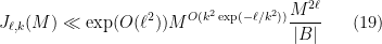
for an absolute constant .
If we apply this theorem with equal to a sufficiently large multiple of , we obtain the required bound  .
.
Actually, Vinogradov proved a slightly weaker estimate than this; the claim above (in a sharper form) was obtained by later refinements of the argument due to Stechkin and Karatsuba. This result has a number of applications beyond that of controlling the Riemann zeta function; for instance it has application to the Waring problem of expressing large natural numbers as the sum of  powers, which we will not discuss further here. The reason for the name “mean value theorem” is that the quantity has a Fourier-analytic interpretation as a mean

of the exponential sum

The estimate (19) should be compared with the lower bound

where the  term comes from the diagonal contribution
  to (17), and the
  term coming from (14) and the Cauchy-Schwarz inequality. Informally, (19) is an assertion that the -fold sum of the discrete curve (13) is somewhat close to being uniformly distributed on . The main conjecture of Vinogradov asserts the near-optimal bound

for any choice of and  . In the recent work of Wooley and Ford-Wooley, an improved version of the congruencing method given below known as efficient congruencing has been developed and used to establish the main conjecture (20) in many cases. See this recent ICM proceedings article of Wooley for a survey of the latest developments in this direction.
We now turn to the proof of the Vinogradov mean value theorem. Since

and , we have  , and so it will suffice to show that

whenever and  is the normalised quantity

which can be viewed as a measure of irregularity of distribution of the quantity  for
for  .
.
We have the extremely crude bound

coming from the fact that there are  choices of , so that

This already establishes the claim when  (say). For
  , what we will do is establish the recursive inequality

whenever and some  ; iterating this
  times and then using (23), we will obtain the claim. Note how it is important here that no powers of are lost in the estimate (24). However, we can be quite generous in losing factors such as
  ,
,  , or
, or  as these are easily absorbed in the
  term. To prove (24), we begin with a technical reduction. For a prime , let us first define a restricted version
  of to be the number of solutions to

with , with  having distinct reductions mod , and
  also having distinct reductions mod . As we are taking to be rather large, one should think of the constraint of having distinct reductions mod to be a mild condition, so that is morally of the same size as . This is confirmed by the following proposition:
Lemma 14 There exists a prime with  such that

The reason why we need the prime to be somewhat comparable to  will be clearer later.
Proof: By definition, is the number of solutions to

with . If the set  has cardinality less than , then there are
  ways to choose the
  , and
, and  ways to choose
  , leading to a contribution of at most
  to . Similarly if
  has cardinality less than . Thus we may restrict attention to the case when and have cardinality at least . By paying a factor of
  , we may then restrict to the case where are all distinct, and are all distinct. In particular, the quantity

is non-zero and has cardinality at most  . In particular, there are at most
  primes larger than that define this quantity. On the other hand, from the prime number theorem we can find
  distinct primes
  in the range
  . We thus see that for each solution to (25) with , distinct, and distinct, there is a
  such that has distinct reductions mod
  , and also has distinct reductions mod , so that this tuple contributes to
  . Thus we have
and the claim follows.
Introducing the normalised quantity

and recalling that , we conclude that

for some prime .
The next step is to analyse the multiplicity properties of the -fold sum  . Clearly we have

where the power sums  are defined by

We recall a classical relation, known as Newton’s identities (or Newton-Girard identities), between these power sums and the elementary symmetric polynomials  , defined for
  by the formula

For instance  ,
,  , and
, and  for all
  . One can also view the
  as essentially being the coefficients of the polynomial
  :
:

Lemma 15 (Newton’s identities) For any , one has the polynomial identity

Thus for instance


Proof: We use the method of generating functions. We rewrite the polynomial identity (27) as
On the other hand, taking logarithmic derivatives we have (as formal power series)
![\displaystyle \frac{d}{dx} [(1-y_1 x) \dots (1-y_k x)] = - (1-y_1 x) \dots (1-y_k x) \sum_{a=1}^k \frac{y_a}{1-y_a x}.](https://s0.wp.com/latex.php?latex=%5Cdisplaystyle+%5Cfrac%7Bd%7D%7Bdx%7D+%5B%281-y_1+x%29+%5Cdots+%281-y_k+x%29%5D+%3D+-+%281-y_1+x%29+%5Cdots+%281-y_k+x%29+%5Csum_%7Ba%3D1%7D%5Ek+%5Cfrac%7By_a%7D%7B1-y_a+x%7D.&bg=ffffff&fg=000000&s=0&c=20201002)
From the geometric series formula we have (as formal power series)

and the claim then follows by equating coefficients.
Corollary 16 If  , then the quantity determines the multiset
  up to permutations. In particular, any element
  of
of  has at most representations of the form
  .
.
Proof: The quantity determines the quantities for . By Newton’s identities and induction, this determines the quantities for , and thus determines the polynomial  . The claim now follows from the unique factorisation of polynomials.
This particular result turns out to not give particularly good bounds on ; the sums are so sparsely distributed that the number of representations of a given (in, say, the box ) is typically zero. However, if we localise “-adically”, by replacing the integers  with the ring
  , we get a more usable result:
Corollary 17 Let be a prime with  . Then any
  has at most representations of the form

with  having distinct reductions mod , where by abuse of notation we localise
  to the ring
  in the obvious fashion.
To put it another way, this corollary asserts that the map  from
from  to is at most -to-one, if one excludes those which do not have distinct reductions mod .
Proof: Suppose we have two representations

with  and
and  each having distinct reductions mod . By Newton’s identities as before, we have
  for (note that as there is no difficulty dividing by for ). Therefore we have the polynomial identity

as polynomials over  . In particular, each
  is a root of and thus must equal one of the
  since the reductions mod are all distinct (and so all but one of the factors
  will be invertible in ). This implies that
  is a permutation of , and the claim follows.
Returning to the integers, and specialising to the range of primes produced by Lemma 14, we conclude
Lemma 18 (Linnik’s lemma) Let be a prime with , and let  . Then the number of solutions to the system

with and  , with having distinct reductions modulo , is at most
  .
.
A version of this lemma also applies for primes outside of the range , but this is basically the range where the lemma is the most efficient. Indeed, probabilistic heuristics suggest that the number of solutions here should be approximately  , which equals
  in the range .
Proof: Each residue class mod  consists of
  residue classes mod
  . Since

it thus suffices (replacing with  different elements of ) to show that for any
  , the number of solutions to the lifted system

with and is at most  . But each residue class mod meets
  in at most representatives, so the claim follows from Corollary 17, crudely bounding by .
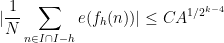
Now we need to consider sums of terms, rather than just terms. Recall that is the number of solutions to
with , with having distinct reductions mod , and also having distinct reductions mod . We also need an even more restricted version  of , which is defined similarly to but with the additional constraint that

Probabilistic heuristics suggest that should be about  as large as . One side of this prediction is confirmed by the following application of Hölder’s inequality:
Lemma 19 (Hölder inequality) We have
In particular, introducing the normalised quantity

we have
Proof: It is easiest to prove this by Fourier-analytic means. Observe that we have the Fourier expansion

where

where the asterisk denotes the restriction to those with distinct reductions modulo and  is the usual dot product
  , and
, and

Similarly, we have

where

Since  , the claim now follows from Hölder’s inequality.
Exercise 20 Find a non-Fourier-analytic proof of the above lemma, based on the Cauchy-Schwarz inequality, in the case when  is a power of two. (Hint: you may wish to generalise the Hölder inequality to one involving the number of solutions
  to systems
  where each
  is drawn from a finite multiset
  (such quantities are known as additive energies of order in the additive combinatorics literature).) For an additional challenge: find a Cauchy-Schwarz proof that works for arbitrary values of .
Next, we use the Linnik lemma and some elementary arguments to bound :
Lemma 21 If , then

where  . In particular, from (22) and (28) we have

Proof: By definition, is the number of solutions to the system

where  , with and each having distinct reductions mod , and also

for some  . From the binomial theorem,
  is a linear transform of
  , so
, so

Writing  and
and  for
for  and some
  , we conclude that

In particular, taking the  coefficient

There are  choices for
  , and then by Linnik’s lemma once are chosen, there are at most
  choices for . Once these are chosen, we still have to select
  subject to a constraint of the form

for some  depending on
  . The number of solutions to this system is

which by the Cauchy-Schwarz inequality is bounded by  . The claim follows.
Combining (26), (29), and (30) we obtain (24) as required.

 , then

whenever
for various intervals
, in the regime
(say). For
, do not try to capture any cancellation and just use the triangle inequality instead.)
, for some (effective) absolute constant
,
depends (ineffectively) on
.


52 comments
Comments feed for this article
7 February, 2015 at 1:23 pm
Anthony
Under equation (1), should it be ‘setting x = 1’ instead of ‘s = 1’?
[Corrected, thanks – T.]
7 February, 2015 at 1:24 pm
Eytan Paldi
In the line below (1), it seems that “ ” should be “
 “.
“.
7 February, 2015 at 1:30 pm
Anthony
…although this then gives s/(s-1), not 1/(s-1).
[The factor of can be absorbed into the
  error; alternatively, one can take
  to be slightly less than
  rather than exactly equal to
  . -T.]
7 February, 2015 at 2:41 pm
Anonymous
My browser can not parse three formulas: the last line of proof of prop 9, two lines above (21), and two lines before lemma 18.
[Corrected, thanks – T.]
7 February, 2015 at 10:16 pm
Anonymous
Use “\colon” instead of “:” for maps. Example: .
.
8 February, 2015 at 1:47 am
Anonymous
In proposition 1, it may be added that is positive.
8 February, 2015 at 4:25 am
Anonymous
In the line above proposition 1, it should be exercise 33 (instead of exercise 34).
[Corrected, thanks – T.]
8 February, 2015 at 7:39 am
Anonymous
In proposition 1, is the implied constant of “ ” (under the supremum) independent of
  ?
?
[Yes – T.]
8 February, 2015 at 1:48 pm
Anonymous
In the line below (3), it should be “derivative of “.
“.
[Corrected, thanks – T.]
9 February, 2015 at 12:55 am
Anonymous
It seems that in proposition 5, the constant can be replaced by any constant
  .
.
[Fair enough; I had thought there was possibly a factor of to take care of, but there isn’t, so I switched the constant to 2 instead. -T.]
9 February, 2015 at 2:01 pm
MrCactu5 (@MonsieurCactus)
I would like to know why the assumptions 3 are reasonable. Proposition 1 seems to say that very far away from the real axis, you can ignore the first terms, and the zeta function is not more oscillatory than the thing you have written down.
9 February, 2015 at 2:18 pm
MrCactu5 (@MonsieurCactus)
Yeah I am definitely not sure. and yet “
 is a polynomial of degree roughly
  “
“
9 February, 2015 at 3:48 pm
Terence Tao
The intuition here is that analytic functions behave like polynomials (a similar philosophy was adopted in https://terrytao.wordpress.com/2014/12/05/245a-supplement-2-a-little-bit-of-complex-and-fourier-analysis/ ), particularly if the radius of convergence is larger than the interval on which one is trying to exploit polynomial-type behaviour. In the case of the function for
for  , the radius of convergence is about
  , which is reflected in the increasing powers of N in the denominator of (3). In particular, the error term in a k-term Taylor expansion is about
  , which can be significantly less than 1 if
  is not too small compared with
  .
.
10 February, 2015 at 2:45 am
Trevor Wooley
Great to see Vinogradov’s methods poularised!
Just a comment that one can make a case now for saying that the main conjecture in Vinogradov’s mean value theorem (your equation (20)) has nearly been proved. By using the multigrade enhancement of my efficient congruencing method, one obtains the main conjecture in the cubic case in full, as well as for arbitrary
  when
when  (and also when
  ). Of course, if one proves (20) for
  , then it follows for all
  , so in a sense we are only
  variables (out of
  ) away from finishing off the conjecture. [There’s an account of this kind of thing in http://arxiv.org/pdf/1404.3508v1.pdf ]
[Reference added – T.]
11 February, 2015 at 2:36 am
Anonymous
It seems that it took more than 20 years to discover the application of Vinogradov mean value theorem (from 1935) to his estimate (theorem 2(ii)).
13 February, 2015 at 10:16 pm
254A, Notes 6: Large values of Dirichlet polynomials, zero density estimates, and primes in short intervals | What's new
[…] the previous set of notes, we studied upper bounds on sums such as for that were valid for all in a given range, such as ; […]
14 February, 2015 at 12:54 pm
Eytan Paldi
In exercise 4, it seems that (in order to use proposition 1), the condition is also needed.
[Fair enough -T.]
17 February, 2015 at 11:46 am
Alastair Irving
I’m slightly confused. IN the Vinogradov estimate theorem 2(ii) you gain by over the trivial bound (the same as in Iwaniec-Kowalski). However, many papers which consider estimating Weyl sums using the Vinogradov method only gain by
  . I understood that one of the consequences of Wooley’s efficient congruencing method is that the
  can be removed. Please can someone explain what I’m missing, in particular why there is no
  in the above theorem?
17 February, 2015 at 11:54 am
Terence Tao
I believe the results you are referring to are for a slightly different exponential sum, namely sums of the form where
where  is a polynomial of degree k. The sums here are a little different:
  where
where  is a smooth function (not a polynomial) which obeys the derivative bound (3) for some
  . In particular the parameter “k” is slightly different in the two contexts. (Both results use Vinogradov’s mean value theorem, but in slightly different ways; in the situation considered in this post, the error exponent
  in the mean value theorem only needs to be less than a small multiple of
  , so one can take
  to be a large multiple of
  , but when dealing with the polynomial sums it seems that the usual methods need this error exponent to be much smaller, like
  , leading to
  being chosen as large as
  .)
.)
1 March, 2015 at 1:13 pm
254A, Supplement 7: Normalised limit profiles of the log-magnitude of the Riemann zeta function (optional) | What's new
[…] limit profiles are known unconditionally, beyond (i)-(iv). For instance, from Exercise 3 of Notes 5 we have as , which implies that any normalised limit profile for is bounded by on the critical […]
6 March, 2015 at 6:31 am
Anonymous
Is it possible to generalize the bilinear estimate (10) to trilinear (or even multilinear) estimates ?
If so, can Vinogradov estimate (6) be improved ?
6 March, 2015 at 11:06 am
Terence Tao
This is theoretically possible, however in practice we have far fewer efficient techniques for dealing with trilinear or higher estimates than for bilinear ones. For instance, bilinear estimates can often be recast as operator norm estimates for a linear operator, for which one can hope to use spectral theory methods to help analyse (e.g. the identity for any natural number
  ). Trilinear estimates correspond to bilinear operators, for which we do not have spectral theory methods at our disposal.
11 December, 2015 at 5:04 am
Anonymous
Is the new decoupling method (used in the proof of Vinogradov main conjecture) seems to have the potential to prove such trilinear (or even higher) estimates?
11 December, 2015 at 8:23 am
Terence Tao
This is potentially possible, and certainly worth exploring. Certainly the Bourgain-Demeter-Guth method relies heavily on multilinear estimates (though not exactly of the type under discussion here).
30 March, 2015 at 12:49 pm
254A, Notes 8: The Hardy-Littlewood circle method and Vinogradov’s theorem | What's new
[…] not be discussed further here, save to note that the Vinogradov mean value theorem (Theorem 13 from Notes 5) and its variants are particularly useful for getting good bounds on ; see for instance the ICM […]
11 September, 2015 at 6:27 am
The Erdos discrepancy problem via the Elliott conjecture | What's new
[…] from the Vinogradov-Korobov zero-free region for (see this previous blog post) it is not difficult to show […]
2 October, 2015 at 10:55 am
valuevar
Dear Terry,
The exponent in Exercise 3(ii) is off (obviously a typo).
[Corrected, thanks – T.]
3 October, 2015 at 5:14 am
valuevar
The error is still there.
3 October, 2015 at 8:26 am
Terence Tao
The min-exponent was corrected to a max. Was there another error you were referring to?
[Edit: see it now, the second should be
  . -T.]
8 December, 2015 at 9:25 am
Terence Tao
News flash: the Vinogradov main conjecture (estimate (20) in the blog post) has now been proven by Bourgain, Demeter, and Guth, using (a modification of) the decoupling restriction theorem of Bourgain and Demeter! http://arxiv.org/abs/1512.01565 Presumably this will impact the best known bounds on the zeta function and the Waring problem, though I don’t know the precise implications in this regard.
8 December, 2015 at 1:39 pm
Anonymous
Is it possible that this has the potential to improve the current (Vinogradov-Korobov) exponent in the PNT error term ?
8 December, 2015 at 1:58 pm
Terence Tao
My initial understanding is that one may need to know how the implied constant in (20) depends on k and epsilon (and maybe also l) in order to get such an improvement. For instance to my knowledge the deep recent results of Wooley have not led to any improvement on Vinogradov-Korobov, in part due to the poor dependence of constants in this regard. But it is plausible that some breakthrough in this direction is now close at hand.
12 December, 2015 at 2:51 pm
Eytan Paldi
In the proof that theorem 11 implies theorem 2(ii), in the sixth line above (12), it is assumed (inside parentheses) that “ is large” but this assumption is not(!) part of theorem 2(ii) (which allows any natural
  ).
).
12 December, 2015 at 6:48 pm
Terence Tao
One can use the van der Corput estimates to assume that k is large (see the first paragraph of Section 2).
13 December, 2015 at 2:16 am
Eytan Paldi
Thanks! (In fact, it seems by first proving (6) for where
where  is sufficiently large, that for the bounded case
  , (6) follows with some smaller
  – as the condition
  is implied by
  ).
).
13 December, 2015 at 6:46 pm
Anonymous
It seems that (defined below (12)) is (in general) a complex number, hence in all the inequalities (below (13)) involving powers of
  (which are also complex),
  should be replaced by
  .
. should be defined as the absolute value of the LHS of (10)).
(or alternatively,
[Corrected, thanks – T.]
16 December, 2015 at 1:50 pm
Anonymous
It seems that the first and second lines in the RHS of the estimate above (14) are due to bounding with
with  (due to Holder inequality) by the Riesz-Thorin interpolation bound between
  and
and  (in terms of
  ).
).
(i.e. it seems that not only Holder inequality is used in this estimate.)
16 December, 2015 at 2:35 pm
Anonymous
I made a mistake (there are no operator norms here), it seems that a generalization of Holder inequality (interpolation between norms) is used.
19 December, 2015 at 1:29 pm
Anonymous
The needed norm interpolation is Littlewood’s inequality (see e.g. in the interpolation section in the Wikipedia article on Holder’s inequality) applied to with
with  and
and  .
.
20 December, 2015 at 4:20 pm
Anonymous
In the third line above (18), should be
  .
.
[Corrected, thanks – T.]
24 December, 2015 at 4:03 am
Anonymous
It seems that the coefficients in (16) are not used in the transition to (18). Hence (for simplicity) they can be eliminated before(16).
24 December, 2015 at 4:44 am
Anonymous
In fact, it is not clear if these coefficients can be eliminated before (16).
26 December, 2015 at 7:52 am
Anonymous
It is interesting to observe that the summations in (14)-(15) are not necessarily restricted to the box (because
  is supported in this box) – this fact is actually used in the application of C-S inequality to get (18).
27 December, 2015 at 2:58 am
Anonymous
In the proof of lemma 12, it seems clearer to remark that the inequality in the line above “and hence” is valid for the above chosen subset of indices that satisfy (9).
[Clarification added, thanks – T.]
27 December, 2015 at 4:43 am
Anonymous
In the proof of lemma 12, it is assumed (in the last two lines) that for some large
  . But this assumption is not(!) present in the statement of lemma 12.
[This bound comes from the ambient hypothesis (12). -T.]
28 March, 2017 at 5:25 pm
Claudeh5
Hello professor Tao,
In “Vinogradov estimate” the first equation (which is on 3 lines) has a small error in the line 3: a square is lost in the integral : |f”(t)/|f'(t)|^2
[Corrected, thanks – T.]
8 July, 2018 at 4:09 am
Anonymous
Dear Prof. Tao,
I’m confused with the last two sentences of the proof of Prop. 6. The size may be $O(AN/T)$? And the bound in Prop. 6 seems too strong comparing with Cor. 8.13 in Iwaniec–Kowalski’s book. Thanks.
1 June, 2019 at 1:11 pm
Sungjin Kim
Dear Professor Tao,
In the Exercise 5 (iii), shouldn’t there be on the right side, not
  ?
?
[Corrected, thanks – T.]
4 September, 2019 at 1:47 pm
254A announcement: Analytic prime number theory | What's new
[…] Bounds for exponential sums […]
5 October, 2023 at 12:41 pm
Anonymous
In the second displayed equation after Prop 1, should be just
  .
.
[The epsilon dependence is needed to absorb the term from the previous display. -T]
6 October, 2023 at 12:40 am
Lior Silberman
Yes — I missed the condition which creates the
  -dependence.
30 January, 2024 at 7:50 am
Anonymous
Dear Terry, you said that pseudorandomness heuristics predict a bound for (2) (which, in particular , implies the Lindelof hypothesis) under the assumption (3) and, if I understand well, also under some more general assumptions. Could you please tell me where I could read more about that and how can one generalize (3) and still expect the bound O(N^{-1/2+epsilon}) to hold? Thank you very much!