
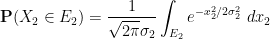
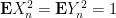
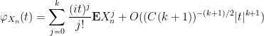
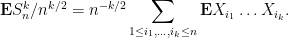
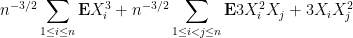
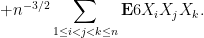
Let 


and

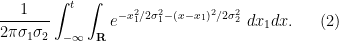
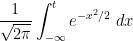
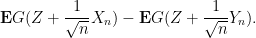
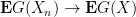
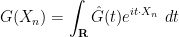
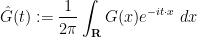
Then, as computed in previous notes, the normalised fluctuation 


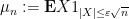
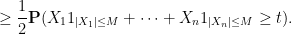
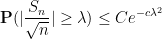
This and Chebyshev’s inequality already indicates that the “typical” size of 


From this and the Paley-Zygmund inequality (Exercise 44 of Notes 1) we also get some lower bound for 
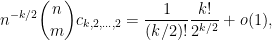
for some absolute constant 


The question remains as to what happens to the ratio
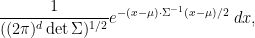
Proposition 1 Let
Proof: Suppose for contradiction that some sequence 


Nevertheless there is an important limit for the ratio
Definition 2 (Vague convergence and convergence in distribution) Let
be a locally compact Hausdorff topological space with the Borel
-algebra. A sequence of finite measures
on
if one has
as
. (Vague convergence is also known as weak convergence, although strictly speaking the terminology weak-* convergence would be more accurate.) A sequence of random variables
taking values in
converge vaguely to the distribution
, or equivalently if
as


One could in principle try to extend this definition beyond the locally compact Hausdorff setting, but certain pathologies can occur when doing so (e.g. failure of the Riesz representation theorem), and we will never need to consider vague convergence in spaces that are not locally compact Hausdorff, so we restrict to this setting for simplicity.
Note that the notion of convergence in distribution depends only on the distribution of the random variables involved. One consequence of this is that convergence in distribution does not produce unique limits: if 

From the dominated convergence theorem (available for both convergence in probability and almost sure convergence) we see that convergence in probability or almost sure convergence implies convergence in distribution. The converse is not true, due to the insensitivity of convergence in distribution to equivalence in distribution; for instance, if
Remark 3 The notion of convergence in distribution is somewhat similar to the notion of convergence in the sense of distributions that arises in distribution theory (discussed for instance in this previous blog post), however strictly speaking the two notions of convergence are distinct and should not be confused with each other, despite the very similar names.
The notion of convergence in distribution simplifies in the case of real scalar random variables:
Proposition 4 Let
- (i)
- (ii)
converges to
for each continuity point
of
(i.e. for all real numbers
at which
is the cumulative distribution function of
Proof: First suppose that 


for every ![{t' \in [t-\delta,t+\delta]}](https://s0.wp.com/latex.php?latex=%7Bt%27+%5Cin+%5Bt-%5Cdelta%2Ct%2B%5Cdelta%5D%7D&bg=ffffff&fg=000000&s=0&c=20201002)


and
Let ![{G: {\bf R} \rightarrow [0,1]}](https://s0.wp.com/latex.php?latex=%7BG%3A+%7B%5Cbf+R%7D+%5Crightarrow+%5B0%2C1%5D%7D&bg=ffffff&fg=000000&s=0&c=20201002)
![{[-2N, t]}](https://s0.wp.com/latex.php?latex=%7B%5B-2N%2C+t%5D%7D&bg=ffffff&fg=000000&s=0&c=20201002)

![{[-N, t-\delta]}](https://s0.wp.com/latex.php?latex=%7B%5B-N%2C+t-%5Cdelta%5D%7D&bg=ffffff&fg=000000&s=0&c=20201002)

and hence

for large enough

A similar argument, replacing 
![{[t,2N]}](https://s0.wp.com/latex.php?latex=%7B%5Bt%2C2N%5D%7D&bg=ffffff&fg=000000&s=0&c=20201002)
![{[t+\delta,N]}](https://s0.wp.com/latex.php?latex=%7B%5Bt%2B%5Cdelta%2CN%5D%7D&bg=ffffff&fg=000000&s=0&c=20201002)

for

for 
Conversely, suppose that 
![{G_\varepsilon(t) = \sum_{i=1}^n c_i 1_{(t_i,t_{i+1}]}}](https://s0.wp.com/latex.php?latex=%7BG_%5Cvarepsilon%28t%29+%3D+%5Csum_%7Bi%3D1%7D%5En+c_i+1_%7B%28t_i%2Ct_%7Bi%2B1%7D%5D%7D%7D&bg=ffffff&fg=000000&s=0&c=20201002)


Similarly for

and on sending
The restriction to continuity points of 


Example 5 For any natural number
, and let
. Then
Example 6 For any natural number
, then
Exercise 7 (Portmanteau theorem) Show that the properties (i) and (ii) in Proposition 4 are also equivalent to the following three statements:
- (iii) One has
for all closed sets
.
- (iv) One has
for all open sets
.
- (v) For any Borel set
whose topological boundary
is such that
, one has
.
(Note: to prove this theorem, you may wish to invoke Urysohn’s lemma. To deduce (iii) from (i), you may wish to start with the case of compact
.)
We can now state the famous central limit theorem:
Theorem 8 (Central limit theorem) Let
and finite non-zero variance
. Let
converges in distribution to a random variable with the standard normal distribution
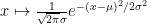
(that is to say, a random variable with probability density function
). Thus, by abuse of notation
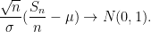
In the normalised case

Using Proposition 4 (and the fact that the cumulative distribution function associated to

as

Informally, one can think of the central limit theorem as asserting that 


The central limit theorem is a basic example of the universality phenomenon in probability – many statistics involving a large system of many independent (or weakly dependent) variables (such as the normalised sums 
We will give several proofs of the central limit theorem in these notes; each of these proofs has their advantages and disadvantages, and can each extend to prove many further results beyond the central limit theorem. We first give Lindeberg’s proof of the central limit theorem, based on exchanging (or swapping) each component 

The following exercise illustrates the power of the central limit theorem, by establishing combinatorial estimates which would otherwise require the use of Stirling’s formula to establish.
Exercise 9 (De Moivre-Laplace theorem) Let
with
, thus
and variance
. Let
.
- (i) Show that
with
. (This is an example of a binomial distribution.)
- (ii) Assume Stirling’s formula
where
is a function of
as
.
The above special case of the central limit theorem was first established by de Moivre and Laplace.


We close this section with some basic facts about convergence of distribution that will be useful in the sequel.
Exercise 10 Let
be sequences of real random variables, and let
be further real random variables.
- (i) If
- (ii) Suppose that
for each
converges in distribution to
if and only if
- (iii) If
such that
for all sufficiently large
- (iv) Show that
and
of
converges almost surely to
- (v) If
is continuous, show that
converges in distribution to
. Generalise this claim to the case when
- (vi) (Slutsky’s theorem) If
converges in distribution to
, and
converges in distribution to
. (Hint: either use (iv), or else use (iii) to control some error terms.) This statement combines particularly well with (i). What happens if
- (vii) (Fatou lemma) If
is continuous, and
.
- (viii) (Bounded convergence) If
.
- (ix) (Dominated convergence) If
almost surely for all
.
For future reference we also mention (but will not prove) Prokhorov’s theorem that gives a partial converse to part (iii) of the above exercise:
Theorem 11 (Prokhorov’s theorem) Let
for all sufficiently large
which converges in distribution to some random variable
The proof of this theorem relies on the Riesz representation theorem, and is beyond the scope of this course; but see for instance Exercise 29 of this previous blog post. (See also the closely related Helly selection theorem, covered in Exercise 30 of the same post.)
— 1. The Lindeberg approach to the central limit theorem —
We now give the Lindeberg argument establishing the central limit theorem. The proof splits into two unrelated components. The first component is to establish the central limit theorem for a single choice of underlying random variable
We begin with the first component of the argument. One could use the Bernoulli distribution from Exercise 9 as the choice of underlying random variable, but a simpler choice of distribution (in the sense that no appeal to Stirling’s formula is required) is the normal distribution
Lemma 12 (Sum of independent Gaussians) Let
be independent real random variables with normal distributions
,
respectively for some
and
. Then
has the normal distribution
.
This is of course consistent with the additivity of mean and variance for independent random variables, given that random variables with the distribution
Proof: By subtracting 


and
for any Borel sets 

for any Borel set 


for any 
We can complete the square using

so on using the identity 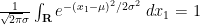


and so 
In the next section we give an alternate proof of the above lemma using the machinery of characteristic functions. A more geometric argument can be given as follows. With the same normalisations as in the above proof, we can write 


From the above lemma we see that if 

Exercise 13 (Probabilistic interpretation of convolution) Let
be measurable functions with
. Define the convolution
of
and
to be
Show that if
are independent real random variables with probability density functions
respectively, then
Now we turn to the general case of the central limit theorem. By subtracting 


as
Let 

as
as
We first establish this claim under the additional simplifying assumption of a finite third moment: 

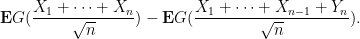
Writing 
To compute this expression we use Taylor expansion. As

where the implied constant depends on

Now for a key point: as the random variable 

The same considerations apply after swapping


But by hypothesis, 

A similar argument (permuting the indices, and replacing some of the 


for all 

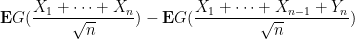
which gives (5). Note how it was important to Taylor expand to at least third order to obtain a total error bound that went to zero, which explains why it is the first two moments 
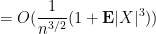
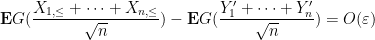
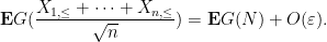
Now we remove the hypothesis of finite third moment. As in the previous set of notes, we use the truncation method, taking advantage of the “room” inherent in the 


Let 


for

and thus
for large enough 


as
Next, we consider the error term
The variable 
As

Taking expectations, and then combining all these estimates, we conclude that

for
The above argument can be generalised to a central limit theorem for certain triangular arrays, known as the Lindeberg central limit theorem:
Exercise 14 (Lindeberg central limit theorem) Let
be a sequence of natural numbers going to infinity in
be jointly independent real random variables of mean zero and finite variance. (We do not require the random variables
to be jointly independent in
be defined by
and assume that
for all
- (i) If one assumes the Lindeberg condition that
as
converge in distribution to a random variable with the normal distribution
- (ii) Show that the Lindeberg condition implies the Feller condition
as

Note that Theorem 8 (after normalising to the mean zero case 


Exercise 15 (Weak Berry-Esséen theorem) Let
- (i) Show that
whenever
notation absolute.
- (ii) Show that
for any


We will strengthen the conclusion of this theorem in Theorem 37 below.
Remark 16 The Lindeberg exchange method explains why the limiting distribution of statistics such as
depend primarily on the first two moments of the component random variables
depend primarily on the first four moments of the matrix components
, if there is a suitable amount of independence between the
We now use the Lindeberg central limit theorem to obtain the converse direction of the Kolmogorov three-series theorem (Exercise 29 of Notes 3).
Exercise 17 (Kolmogorov three-series theorem, converse direction) Let
is almost surely convergent (i.e., the partial sums are almost surely convergent), and let
.
- (i) Show that
is finite. (Hint: argue by contradiction and use the second Borel-Cantelli lemma.)
- (ii) Show that
is finite. (Hint: first use (i) and the Borel-Cantelli lemma to reduce to the case where
almost surely. If
is infinite, use Exercise 14 to show that
converges in distribution to a standard normal distribution, and use this to contradict the almost sure convergence of
- (iii) Show that the series
is convergent. (Hint: reduce as before to the case where
.)
— 2. The Fourier-analytic approach to the central limit theorem —
Let us now give the standard Fourier-analytic proof of the central limit theorem. Given any real random variable 
Equivalently, 

Example 18 The signed Bernoulli distribution, which takes the values
and
with probabilities of
.
Most of the standard random variables in probability have characteristic functions that are quite simple and explicit. For the purposes of proving the central limit theorem, the most important such explicit form of the characteristic function is of the normal distribution:
Exercise 19 Show that the normal distribution
.
We record the explicit characteristic functions of some other standard distributions:
Exercise 20 Let
, and let
, thus
. Show that
for all
Exercise 21 Let
. Show that
for all non-zero
Exercise 22 Let
and
, and let
, which means that
. Show that
for all
The characteristic function is clearly bounded in magnitude by
Exercise 23 (Riemann-Lebesgue lemma) Show that if
as
. (Hint: first show the claim when
norm by such finite linear combinations.) Note from Example 18 that the claim can fail if
Exercise 24 Show that the characteristic function
Let
which thus interprets the characteristic function of a real random variable
Exercise 25 (Taylor expansion of characteristic function) Let
moment for some
. Show that
times continuously differentiable, with
for all
. Conclude in particular the partial Taylor expansion
where
is a quantity that goes to zero as
, times
.

Exercise 26 Let
such that
for all

Note that the characteristic function depends only on the distribution of 

Theorem 27 (Lévy continuity theorem, special case) Let
- (i)
converges pointwise to
- (ii)
Proof: The implication of (i) from (ii) is immediate from (6) and Exercise 10(viii).
Now suppose that (i) holds, and we wish to show that (ii) holds. We need to show that
whenever
where
is Schwartz, and is in particular absolutely integrable (see e.g. these lecture notes of mine). From the Fubini-Tonelli theorem, we thus have

and similarly for
Remark 28 Setting
for all
There is one subtlety with the Lévy continuity theorem: it is possible for a sequence 


Exercise 29 (Lévy’s continuity theorem, full version) Let
. Show that the following are equivalent:
- (i)
- (ii)
- (iii)
- (iv)
Hint: To get from (ii) to the other conclusions, use Theorem 11 and Theorem 27. To get back to (ii) from (i), use (8) for a suitable Schwartz function
Remark 30 Lévy’s continuity theorem is very similar in spirit to Weyl’s criterion in equidistribution theory.
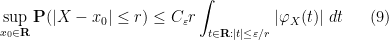
Exercise 31 (Esséen concentration inequality) Let
. Then for any
,
for some constant
depending only on
.
In Fourier analysis, we learn that the Fourier transform is a particularly well-suited tool for studying convolutions. The probability theory analogue of this fact is that characteristic functions are a particularly well-suited tool for studying sums of independent random variables. More precisely, we have
Exercise 32 (Fourier identities) Let
for all
. Also, for any scalar
, one has
and more generally, for any linear transformation
, one has

Remark 33 Note that this identity (10), combined with Exercise 19 and Remark 28, gives a quick alternate proof of Lemma 12.
In particular, we have the simple relationship

that describes the characteristic function of
We now have enough machinery to give a quick proof of the central limit theorem:
Proof: (Fourier proof of Theorem 8) We may normalise
for sufficiently small

for sufficiently small

as 
The above machinery extends without difficulty to vector-valued random variables 


We leave the routine extension of the above results and proofs to the higher dimensional case to the reader. Most interesting is what happens to the central limit theorem:
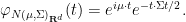
Exercise 34 (Vector-valued central limit theorem) Let
be a random variable taking values in
to be the
matrix
whose
entry is the covariance
.
- Show that the covariance matrix is positive semi-definite real symmetric.
- Conversely, given any positive definite real symmetric
, show that the multivariate normal distribution
, given by the absolutely continuous measure
has mean
How would one define the normal distribution
- If
is the sum of
, show that
converges in distribution to
. (For this exercise, you may assume without proof that the Lévy continuity theorem extends to
Exercise 35 (Complex central limit theorem) Let
, whose real and imaginary parts have variance
and covariance
be iid copies of
converge in distribution to the standard complex gaussian
, defined as the measure
with
for Borel
, where
is Lebesgue measure on
in the usual fashion).

Exercise 36 Use characteristic functions and the truncation argument to give an alternate proof of the Lindeberg central limit theorem (Theorem 14).
A more sophisticated version of the Fourier-analytic method gives a more quantitative form of the central limit theorem, namely the Berry-Esséen theorem.
Theorem 37 (Berry-Esséen theorem) Let
, where
are iid copies of
uniformly for all
, where

Proof: (Optional) Write 
for all 

Let 

![{[-c,c]}](https://s0.wp.com/latex.php?latex=%7B%5B-c%2Cc%5D%7D&bg=ffffff&fg=000000&s=0&c=20201002)

![{[-c/2,c/2]}](https://s0.wp.com/latex.php?latex=%7B%5B-c%2F2%2Cc%2F2%5D%7D&bg=ffffff&fg=000000&s=0&c=20201002)
Let 
![{1_{(-\infty,0]}}](https://s0.wp.com/latex.php?latex=%7B1_%7B%28-%5Cinfty%2C0%5D%7D%7D&bg=ffffff&fg=000000&s=0&c=20201002)
![\displaystyle \psi(x) := \int_{\bf R} 1_{(-\infty,0]}(x - \varepsilon y) \eta(y)\ dy](https://s0.wp.com/latex.php?latex=%5Cdisplaystyle++%5Cpsi%28x%29+%3A%3D+%5Cint_%7B%5Cbf+R%7D+1_%7B%28-%5Cinfty%2C0%5D%7D%28x+-+%5Cvarepsilon+y%29+%5Ceta%28y%29%5C+dy&bg=ffffff&fg=000000&s=0&c=20201002)

Observe that 
![\displaystyle \psi(x) = 1_{(-\infty,0]}(x) + O_\eta( (1+|x|/\varepsilon)^{-100} ) \ \ \ \ \ (14)](https://s0.wp.com/latex.php?latex=%5Cdisplaystyle++%5Cpsi%28x%29+%3D+1_%7B%28-%5Cinfty%2C0%5D%7D%28x%29+%2B+O_%5Ceta%28+%281%2B%7Cx%7C%2F%5Cvarepsilon%29%5E%7B-100%7D+%29+%5C+%5C+%5C+%5C+%5C+%2814%29&bg=ffffff&fg=000000&s=0&c=20201002)
(say) for any 
We claim that it suffices to show that
for every 


for any 

Also, ![{[a,a+\varepsilon]}](https://s0.wp.com/latex.php?latex=%7B%5Ba%2Ca%2B%5Cvarepsilon%5D%7D&bg=ffffff&fg=000000&s=0&c=20201002)
![\displaystyle {\bf E} ( \frac{S_n}{\sqrt{n}} \in [a,a+\varepsilon] ) = O_\eta(\varepsilon) \ \ \ \ \ (16)](https://s0.wp.com/latex.php?latex=%5Cdisplaystyle++%7B%5Cbf+E%7D+%28+%5Cfrac%7BS_n%7D%7B%5Csqrt%7Bn%7D%7D+%5Cin+%5Ba%2Ca%2B%5Cvarepsilon%5D+%29+%3D+O_%5Ceta%28%5Cvarepsilon%29+%5C+%5C+%5C+%5C+%5C+%2816%29&bg=ffffff&fg=000000&s=0&c=20201002)
for all real

as can be seen by covering the real line by intervals ![{[a+j\varepsilon, a+(j+1)\varepsilon)]}](https://s0.wp.com/latex.php?latex=%7B%5Ba%2Bj%5Cvarepsilon%2C+a%2B%28j%2B1%29%5Cvarepsilon%29%5D%7D&bg=ffffff&fg=000000&s=0&c=20201002)
![\displaystyle {\bf E} \psi(\frac{S_n}{\sqrt{n}} - a) = {\bf E} 1{(-\infty,0]}(\frac{S_n}{\sqrt{n}} - a) + O_\eta(\varepsilon).](https://s0.wp.com/latex.php?latex=%5Cdisplaystyle++%7B%5Cbf+E%7D+%5Cpsi%28%5Cfrac%7BS_n%7D%7B%5Csqrt%7Bn%7D%7D+-+a%29+%3D+%7B%5Cbf+E%7D+1%7B%28-%5Cinfty%2C0%5D%7D%28%5Cfrac%7BS_n%7D%7B%5Csqrt%7Bn%7D%7D+-+a%29+%2B+O_%5Ceta%28%5Cvarepsilon%29.&bg=ffffff&fg=000000&s=0&c=20201002)
A similar argument gives
![\displaystyle {\bf E} \psi(N - a) = {\bf E} 1{(-\infty,0]}(N - a) + O_\eta(\varepsilon),](https://s0.wp.com/latex.php?latex=%5Cdisplaystyle++%7B%5Cbf+E%7D+%5Cpsi%28N+-+a%29+%3D+%7B%5Cbf+E%7D+1%7B%28-%5Cinfty%2C0%5D%7D%28N+-+a%29+%2B+O_%5Ceta%28%5Cvarepsilon%29%2C&bg=ffffff&fg=000000&s=0&c=20201002)
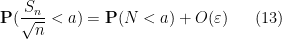
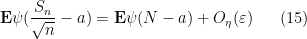
and (13) then follows from (15).
It remains to establish (15). We write

(with the expression in the limit being uniformly bounded) and
to conclude (after applying Fubini’s theorem) that
using the compact support of 

By the fundamental theorem of calculus we have 


and so it suffices to show that
uniformly in 
From Taylor expansion we have

for any

and in particular

if 

if 


(say) if
Exercise 38 Show that the error terms in Theorem 37 are sharp (up to constants) when
with probability
Exercise 39 Let
The following exercise shows that the central limit theorem fails when the variance is infinite.
Exercise 40 Let
- (i) In this part we assume that
have the same distribution. Show that for any
and
,
(Hint: relate both sides of this inequality to the probability of the event that
and
, using the symmetry of the situation.)
- (ii) If
will have arbitrarily large variance as
can be made arbitrarily small by taking
large enough. For a large threshold
) to obtain a contradiction.
- (iii) Generalise (ii) by removing the hypothesis that
, where
is an independent copy of
Exercise 41
- (i) If
and that
(Hint: first establish the Taylor bounds
and
.)
- (ii) Establish the pointwise inequality
whenever
are complex numbers in the disk
.
- (iii) Suppose that for each
are jointly independent real random variables of mean zero and finite variance, obeying the uniform bound
for all
and some
going to zero as
as
. If
, use (i) and (ii) to show that
as
- (iv) Use (iii) and a truncation argument to give an alternate proof of the Lindeberg central limit theorem (Theorem 14). (Note: one has to address the issue that truncating a random variable may alter its mean slightly.)


— 3. The moment method —
The above Fourier-analytic proof of the central limit theorem is one of the quickest (and slickest) proofs available for this theorem, and is accordingly the “standard” proof given in probability textbooks. However, it relies quite heavily on the Fourier-analytic identities in Exercise 32, which in turn are extremely dependent on both the commutative nature of the situation (as it uses the identity 

The most elementary (but still remarkably effective) method available in this regard is the moment method, which we have already used in previous notes. In principle, this method is equivalent to the Fourier method, through the identity (7); but in practice, the moment method proofs tend to look somewhat different than the Fourier-analytic ones, and it is often more apparent how to modify them to non-independent or non-commutative settings.
We first need an analogue of the Lévy continuity theorem. Here we encounter a technical issue: whereas the Fourier phases 

Exercise 42 (Subgaussian random variables) Let
- (i) There exist
such that
for all
.
- (ii) There exist
such that
for all
- (iii) There exist
such that
for all
Furthermore, show that if (i) holds for some
, then (ii) holds for
depending only on
is known as the moment generating function of
Exercise 43 Use the truncation method to show that in order to prove the central limit theorem (Theorem 8), it suffices to do so in the case when the underlying random variable
Once we restrict to the subgaussian case, we have an analogue of the Lévy continuity theorem:
Theorem 44 (Moment continuity theorem) Let
,
converges pointwise to
. Then
Proof: Let 

for some

when
uniformly in

Then letting 


We remark that in place of Stirling’s formula, one can use the cruder lower bound 


Remark 45 One corollary of Theorem 44 is that the distribution of a subgaussian random variable is uniquely determined by its moments (actually, this could already be deduced from Exercise 26 and Remark 28). The situation can fail for distributions with slower tails, for much the same reason that a smooth function is not determined by its derivatives at one point if that function is not analytic.
The Fourier inversion formula provides an easy way to recover the distribution from the characteristic function. Recovering a distribution from its moments is more difficult, and sometimes requires tools such as analytic continuation; this problem is known as the inverse moment problem and will not be discussed here.
Exercise 46 (Converse direction of moment continuity theorem) Let
for all
We now give the moment method proof of the central limit theorem. As discussed above we may assume without loss of generality that

for all 

The moments 

To understand this expression, let us first look at some small values of
- For
, this expression is trivially
- For
, this expression is trivially
- For
, we can split this expression into the diagonal and off-diagonal components:
Each summand in the first sum is
is
- For
, we have a similar expansion
The summands in the latter two sums vanish because of the (joint) independence and mean zero hypotheses. The summands in the first sum need not vanish, but are
, so the first term is
, which is asymptotically negligible, so the third moment
goes to
- For
, the expansion becomes quite complicated:
Again, most terms vanish, except for the first sum, which is
and is asymptotically negligible, and the sum
, which by the independence and unit variance assumptions works out to
. Thus the fourth moment
goes to
(as it should).


Now we tackle the general case. Ordering the indices 


where 

The total number of such terms depends only on 
As we already saw from the small 


On the other hand, the total number of summands in (18) is clearly at most 


and the main term is happily equal to the moment
Exercise 47 (Chernoff bound) Let
- (i) Show that there exist
such that
for all
for all
; for
, use the Taylor approximation
.)
- (ii) Conclude the Chernoff bound
for some
, and all
.
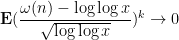
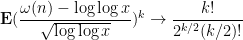
Exercise 48 (Erdös-Kac theorem) For any natural number
, let
, and let
- (i) Show that for any
as
if
as
by
, using Mertens’ theorem and induction on
as being approximately independent and approximately of mean zero.)
- (ii) Establish the Erdös-Kac theorem
as
.
Informally, the Erdös-Kac theorem asserts that
for “random”

72 comments
Comments feed for this article
2 November, 2015 at 7:56 pm
Anonymous
may want to add “275A – probability theory” in the tags
[Added, thanks – T.]
3 November, 2015 at 5:46 am
Anonymous
In theorem 36, the assumption is not really needed (since otherwise (11) holds trivially!)
[Assumption removed, thanks – T.]
3 November, 2015 at 11:07 am
Anonymous
You should use instead of
  and $\cdots$, resp.
3 November, 2015 at 7:21 pm
Anonymous
In exercise 13(ii), “ ” is in fact “
 “, and the expectation should be dependent on the index
  .
.
[Corrected, thanks – T.]
4 November, 2015 at 9:09 am
Anonymous
According to the Wikipedia articles on the CLT and the Berry-Esseen theorem:
1. The term “central limit theorem” (in German) was first used by Polya (in 1920) where the word “central” is due to its central importance in probability theory. The later interpretation of “central” in the sense that the CLT describes the behaviour of the distribution near its center is (according to Le Cam) due to the French school on probability.
2. The best implied constant in the error term in 11, is lower-bounded by (Esseen, 1956) and upper-bounded by
  (Shevtsova, 2011).
4 November, 2015 at 9:46 am
Anonymous
In the proof of Theorem 26 you briefly switch to $R^d$
[Corrected, thanks – T.]
4 November, 2015 at 9:57 am
Anonymous
A useful lemma is that if $X_n$ converge in distribution they can be coupled to converge almost surely. This is also an instructive alternate approach to the second direction in Proposition 4.
[This was the intention of Exercise 10(iv), though I had previously only asked for convergence in probability, and have now strengthened the conclusion. -T.]
4 November, 2015 at 11:18 am
Anonymous
It seems that exercise 10(vi) generalizes Slutsky’s theorem (which deals with a degenerate(!) limit ), but in the Wikipedia article on Slutsky’s theorem (according to the second note) it is claimed that the requirement that
  is degenerate(!) is important (the theorem is not (!) valid in general for a non-degenerate limit
  ) – is this claim true?
[Oops, this was an error – the exercise has now been corrected. -T.]
5 November, 2015 at 6:52 am
Anonymous
Exercise 9, definition of distribution at the beginning has typo.
[Corrected, thanks – T.]
5 November, 2015 at 9:45 am
John Mangual
The Lindberg approach is related to the “renormalization group approach”, as I learned from Yakov Sinai.
However, I couldn’t not reconcile the discussions of RG in hep-th and the discussion in the probability textbook.
5 November, 2015 at 12:21 pm
Joop de Maat
A typo (“equvialence” before Remark 3) and a question: How exactly are the two notions of distributions from Remark 3 similar ? You only indicated in what the where different, not in what they are alike.
5 November, 2015 at 12:54 pm
Terence Tao
Thanks for the correction! The similarity is both notions of convergence require testing against “nice” functions (continuous compactly supported functions in the case of convergence in distribution, and smooth compactly supported functions in the case of convergence in the sense of distributions). In particular, it is true that a sequence of random variables converge in distribution to a random variable
  if and only if the probability measures
  converge in the sense of distributions to
  . (But once one leaves the setting of probability measures, one can have more exotic distributions as the distributional limit, e.g. derivatives of delta functions.)
14 November, 2015 at 11:59 am
Venky
In the Lindberg approach, I was trying to see where the Gaussian nature of the pdf of Y_i is important other than (3). Can one say that an implication of CLT is that the Gaussian pdf is the only pdf that preserves its functional form over countable addition of independent variables? Great notes, thanks.
14 November, 2015 at 12:20 pm
Terence Tao
Yes, the gaussian is the only finite-variance stable law, and the Lindeberg argument explains why there can be at most one such law. (But there are other stable laws in the infinite variance case, which lie outside of the reach of the CLT: for instance, the Cauchy distribution is also stable.)
14 November, 2015 at 4:35 pm
Anonymous
I have a question on the Example 5, we have known that Xn converges to X in distribution, where Xn is uniform distributed on {1/n, 2/n, …, n/n} and X is uniform[0,1]. How can we check that if Xn converges to X in prob?
14 November, 2015 at 6:49 pm
Terence Tao
This is not possible from the information given, because we do not know the joint distribution of , only the individual distributions of
  and
and  ; the joint distribution is irrelevant for the question of whether there is convergence in distribution, but is very relevant for convergence in probability For instance,
  could be
  rounded up to the next multiple of
  , in which case
  converges to
  in probability (and almost surely). Or,
  could be independent of
  , in which case it will not converge in probability or almost surely to
  .
.
18 November, 2015 at 3:42 pm
Terence Tao
There appears to be a strange issue with one of the wordpress LaTeX renderers right now, as some simple expressions such as are not rendering properly while others such as
  are fine. For those in the class following the notes online, a temporary workaround is to hover one’s mouse over the improperly rendered images to see the uncompiled LaTeX. I do not seem to be able to fix the issue on my end, but I’m hoping that the problem will resolve itself shortly (at which point I will remove this comment).
19 November, 2015 at 8:25 am
Terence Tao
OK, the problem seems to be that as of about 24 hours ago, wordpress has become unable to render any latex fragment that it has not previously rendered, presumably due to the machine that does all the new renderings being somehow offline. I’d be interested to see if other wordpress.com sites are having the same issue, in which case it would make sense to report it. In the meantime, I’ve rolled back these notes to an earlier version for now to avoid the rendering errors. [Update: it now appears that the issue is affecting all wordpress.com blogs, and has been reported. -T.]
19 November, 2015 at 11:38 am
ianmarqz
I have the same problem of well rendering : ( sample: https://juanmarqz.wordpress.com/about/sum-of-reciprocals/
19 November, 2015 at 2:51 pm
275A, Notes 5: Variants of the central limit theorem | What's new
[…] the previous set of notes we established the central limit theorem, which we formulate here as […]
23 November, 2015 at 7:44 pm
Dillon
The characteristic function for a uniform distribution on an interval (Exercise 21) is missing an in the denominator. Also some of the preceding exercises still say
  for the characteristic function where
  would be more consistent.
[Corrected, thanks – T.]
24 November, 2015 at 6:48 pm
Anonymous
In exercise 10 (vii), should it be liminf EG(X_n)>= EG(X)?
[Corrected, thanks – T.]
30 November, 2015 at 3:48 am
Anonymous
‘non-engative’ should be ‘non-negative’ (search and replace time)
[Corrected, thanks – T.]
30 November, 2015 at 4:02 am
Anonymous
‘Levi continuity theorem’ should be ‘Lévy continuity theorem’ (search and replace again)
[Corrected, thanks – T.]
2 December, 2015 at 3:24 am
jura05
thank you for these lectures!
 and apply it to X=S_n/sqrt{n}-a, Y=N-a
some typos:
– formula after (14) – missing term O(.)
– before (15): instead of “below by 1/2 on [0,eps]” should be “below by 1/2 on [a,a+eps]”
– proof of (14) goes for the special case a=0; although there is no difference.. maybe it is convenient to write a general bound
[Corrected, thanks – T.]
30 May, 2016 at 12:56 am
Anonymous
Thanks for the great notes. Small typos:
1. inequality (2) and the following equation are missing a square in the $(x-x_1)^2$ term.
2. Closed bracket missing in Ex 17 (ii)
3. Ex 17 (iii), the indicator function doesn’t appear correctly.
[Corrected, thanks – T.]
30 May, 2016 at 7:56 am
Anonymous
What is known about the convergence rate in Erdos-Kac theorem?
30 May, 2016 at 10:49 am
Terence Tao
I think this paper by Harper represents the current state of the art: http://www.ams.org/mathscinet-getitem?mr=2507311
2 October, 2016 at 6:53 am
Anonymous
In Exercise 14, for each ,
,  are jointly independent. What do you mean by “We do not require the random variables
  to be jointly independent in
  “? Would you illustrate by giving an example that what could be dependent here?
[For instance, we do not require the tuple to be independent of
  . -T.]
4 October, 2016 at 5:55 am
Anonymous
In Exercise 25, can one avoid calculating the -th derivative of
  by just directly integrating the Taylor expansion of
  ?
?
[This should work also, as long as one is careful with estimating error terms – T.]
4 October, 2016 at 6:17 am
Anonymous
For Exercise 19, all the textbooks I have seen use the contour integrals. Can one do it with other methods than the one in complex analysis?
[One such method begins by observing that the pdf of the normal distribution obeys an ODE which then translates to an ODE for the characteristic function (cf. Stein’s method). -T]
4 October, 2016 at 6:23 am
Anonymous
In the Fourier proof of Theorem 8, would you elaborate the “equivalently” part? Is the parenthesis a typo there?
[We are using the Taylor approximation for small
  (specifically,
  ). -T.]
4 October, 2016 at 7:09 pm
Anonymous
By direct substitution, I got

For fixed $t$, when taking the limit, how do you get rid of the little o term?
4 October, 2016 at 9:26 pm
Terence Tao
The asymptotic notation here is with respect to the limit
  , rather than
  ,so the
  term goes to zero in the limit when
  is fixed and
  goes to infinity. (By the way, I corrected a typo in my previous answer, in which I had omitted a factor of
  in the choice of
  .)
.)
5 October, 2016 at 1:00 pm
Anonymous
In Exercise 14, what is the intuition of the Lindeberg condition?

Why would one expect such a condition implies the desired result?
6 October, 2016 at 11:40 am
Terence Tao
The central limit theorem can fail if there is a significant probability that one of the summands is so large that it is comparable to the total standard deviation
  . The Lindeberg condition is basically an assertion that these sort of outlier events are vanishingly rare (and their contribution to the sum has vanishingly small variance) in the limit
  .
.
6 October, 2016 at 6:03 pm
Anonymous
I saw Billingsley in his Probability and Measure proves Remark 28 by proving the inversion formula:
If the probability measure has characteristic function
  and $\mu\{a\}=\mu\{b\}=0$, then
![\displaystyle \mu(a,b]=\lim_{T\to\infty}\frac{1}{2\pi}\int_{-T}^T\frac{e^{-ita}-e^{-itb}}{it}\ dt.](https://s0.wp.com/latex.php?latex=%5Cdisplaystyle+%5Cmu%28a%2Cb%5D%3D%5Clim_%7BT%5Cto%5Cinfty%7D%5Cfrac%7B1%7D%7B2%5Cpi%7D%5Cint_%7B-T%7D%5ET%5Cfrac%7Be%5E%7B-ita%7D-e%5E%7B-itb%7D%7D%7Bit%7D%5C+dt.+&bg=ffffff&fg=545454&s=0&c=20201002)
This approach looks rather different from the one in the proof of Theorem 27, which uses the Schwartz functions and is much shorter. What makes the Schwartz function-approach faster and is it hinted somewhere that these two approaches are essentially the same?
8 October, 2016 at 4:58 am
Anonymous
Ah, the inversion formula should be
![\displaystyle \mu(a,b]=\lim_{T\to\infty}\frac{1}{2\pi}\int_{-T}^T\frac{e^{-ita}-e^{-itb}}{it}\varphi(t) dt.](https://s0.wp.com/latex.php?latex=%5Cdisplaystyle+%5Cmu%28a%2Cb%5D%3D%5Clim_%7BT%5Cto%5Cinfty%7D%5Cfrac%7B1%7D%7B2%5Cpi%7D%5Cint_%7B-T%7D%5ET%5Cfrac%7Be%5E%7B-ita%7D-e%5E%7B-itb%7D%7D%7Bit%7D%5Cvarphi%28t%29+dt.+&bg=ffffff&fg=545454&s=0&c=20201002)
Actually, the proof of the inversion formula is not that long. The key step is just exchanging the integral using Fubini and taking the limit. Still it looks rather different from the Schwartz-function-approach.
8 October, 2016 at 8:40 am
Terence Tao
Basically the difference lies in the use of the smoothing sums technique: replacing a rough cutoff such as![1_{[a,b]}](https://s0.wp.com/latex.php?latex=1_%7B%5Ba%2Cb%5D%7D&bg=ffffff&fg=545454&s=0&c=20201002) with a smoother cutoff in order to enjoy better decay of the Fourier transform. The price one pays for this is that the formulae become a little less explicit, possibly leading to worse quantitative bounds in some cases, but in many applications this sort of loss is acceptable.
with a smoother cutoff in order to enjoy better decay of the Fourier transform. The price one pays for this is that the formulae become a little less explicit, possibly leading to worse quantitative bounds in some cases, but in many applications this sort of loss is acceptable.
12 October, 2016 at 5:57 pm
Anonymous
In theorem 11, can we replace random variables with random vectors?
[Yes; see for instance the linked exercise. -T.]
13 October, 2016 at 6:55 pm
Anonymous
Also for Proposition 4 and Exercise 7 one can have random vectors instead? I’m wondering if i missed reading some of the notes about the random vector part or it is just trivial generalization.
14 October, 2016 at 6:37 pm
Terence Tao
If one deletes (ii) then the remaining claims are equivalent in the vector-valued case. But it is not clear to me whether there is an analogue for (ii) in the vector-valued case (one has to define the cumulative distribution function properly, and specify exactly what a “point of continuity” would mean for that function); the proof given is restricted to the scalar case.
14 October, 2016 at 6:57 pm
Anonymous
https://en.wikipedia.org/wiki/Cumulative_distribution_function#Multivariate_case
13 October, 2016 at 6:26 pm
Anonymous
In Exercise 7, do you have a hint for (v) —>(i)? I don’t have any idea why the boundary of would have anything to do with continuity of a function.
[Consider sets of the form
 ![E = (-\infty,t]](https://s0.wp.com/latex.php?latex=E+%3D+%28-%5Cinfty%2Ct%5D&bg=ffffff&fg=545454&s=0&c=20201002) . -T.]
. -T.]
13 October, 2016 at 6:52 pm
Anonymous
In the proof of Proposition 4, is a typo? Likewise for several others?
[Corrected, thanks – T.]
22 May, 2017 at 5:55 pm
Quantitative continuity estimates | What's new
[…] starting point for the Lindeberg exchange method in probability theory, discussed for instance in this previous post. The identity in (ii) can also be used in the Lindeberg exchange method; the terms in the […]
25 June, 2017 at 4:51 pm
Discotech
In exercise 35, should the exponent have a $\pi$? I think maybe it should not. Unless I’m misunderstanding the meaning of the Lebesgue integral over the complex plane, the measure defined isn’t normalized to 1.
In the hint on exercise 40, do you mean to refer to the probability $P( X_1 1_{|X_1|>M} + \dots + X_n 1_{|X_d|>M} \geq 0)$ (greater than signs instead of less than signs)?
[Corrected, thanks – T.]
26 October, 2018 at 4:05 am
Anonymous
In Slutsky’s theorem, can one relax the condition regarding the convergence of to be convergence in distribution?
27 October, 2018 at 9:03 am
Terence Tao
When the limit is deterministic, convergence in distribution is the same as convergence in probability.
20 February, 2019 at 2:46 pm
haonanz
Hello Prof. Tao, I have a question regard Exercise 7 prove ii) => v). I am thinking if I could use sigma algebra like proof. I believe the difficulty comes from the fact we have only convergence at continuity point. If we assume it’s true for all t, then I think I can show that the set of E satisfy this property is closed under countable union and countable closure), then use the fact Borel sets are the smallest sigma algebra generated by the half-intervals to complete the proof. I wonder the fact we know those discontinuity is at most countably many points can somehow be used to show this generated sigma algebra still contains the half-intervals thus the borel set.
21 February, 2019 at 8:48 am
Terence Tao
I’m not sure a sigma algebra approach will be easy to execute, because the set of Borel sets with
with  of measure zero is not closed under countable union or countable intersection. (The strategy I had in mind instead is to approximate
  by its interior and its exterior and use (iii), (iv).)
23 February, 2019 at 7:06 am
haonanz
A follow up question regard proving i)=>iii), I can prove the claim for the compact case using upper approximation of a CTS and compact supported function. Do you mind providing hint on how can I extend this to the closed case? Thanks again!
23 February, 2019 at 8:12 am
Terence Tao
Show that for large , the probability
  is close to 1, then show that the probability
  is close to 1 for large
  , thus the probability
  is small.
6 November, 2019 at 3:54 am
anonymous
There should be a $k_n$ instead of $n$ in point (ii) of exercise 14.
[Corrected, thanks – T]
18 April, 2020 at 2:07 pm
Anonymous
Let be iid Bernoulli(
 ) random variables, that is,
  and
and  .
.
Let
where .
.
Show that and determine
  .
.
How can we prove this by using some elementary tools?
24 December, 2020 at 3:43 am
Aditya Guha Roy
You may try to solve it using the central limit theorem and Slutsky’s theorem. I have not done this very exercise, but it seems that this can be done by using these tools. Try it and let us know here.
1 January, 2021 at 8:37 pm
N is a number
Yes that would work. I just checked it.
23 December, 2020 at 4:59 am
Aditya Guha Roy
On line number 22 of these notes, you have written about applying Paley Zygmund inequality to get the mentioned lower bound.
I think there is a typo in labelling it as Exercise 42 of Notes 1 ; it should be Exercise 44 of Notes 1.
[Corrected, thanks – T.]
1 January, 2021 at 6:01 am
N is a number
In Exercise 19, we see that from the definition of characteristic function it suffices to show that the result holds when and
and  Now that calls for showing
 ![\mathbf{E} [ e^{i tX} ] = e^{-t^2 / 2}](https://s0.wp.com/latex.php?latex=%5Cmathbf%7BE%7D+%5B+e%5E%7Bi+tX%7D+%5D+%3D+e%5E%7B-t%5E2+%2F+2%7D&bg=ffffff&fg=545454&s=0&c=20201002) for all complex numbers
for all complex numbers  Now rewriting the LHS as an integral one has a holomorphic function on the LHS and the RHS is also a holomorphic function. Now, one can prove this identity for the case when
  is purely imaginary so that
  is purely real by a direct evaluation of the integral which appears on the LHS.
Now, using the fact that non-trivial holomorphic maps have isolated zeroes, and identifying that the holomorphic map LHS – RHS is zero identically on the imaginary axis, one concludes that the identity holds for all complex numbers
Is that correct ?
[Sure, this works. One can also compute the integral for arbitrary by completing the square and contour shifting instead of relying on analytic continuation. -T]
1 January, 2021 at 9:01 pm
Aditya Guha Roy
I think to show that![\mathbf{E} [ e^{it X} ]](https://s0.wp.com/latex.php?latex=%5Cmathbf%7BE%7D+%5B+e%5E%7Bit+X%7D+%5D&bg=ffffff&fg=545454&s=0&c=20201002) is holomorphic over
is holomorphic over  , an easy way is to notice that it is the derivative of the holomorphic map
 ![t \mapsto \mathbf{E} [ X e^{itX}]](https://s0.wp.com/latex.php?latex=t+%5Cmapsto+%5Cmathbf%7BE%7D+%5B+X+e%5E%7BitX%7D%5D&bg=ffffff&fg=545454&s=0&c=20201002) and hence the former must also be holomorphic.
and hence the former must also be holomorphic.
1 January, 2021 at 9:04 pm
Aditya Guha Roy
Filling a gap in my previous comment: we need to notice that we can interchange the derivative and expectation, thanks to Lebesgue’s dominated convergence theorem.
1 January, 2021 at 8:34 pm
N is a number
Prof. Tao in lines 4-5 of the proof of Proposition 1 you have cited Theorem 24 from Notes 1. I think you wanted to cite Theorem 25 from Notes 1 (since here we have the premises satisfied for ).
).
[Corrected, thanks – T.]
17 March, 2021 at 2:46 pm
Orestis Plevrakis
I tried to prove Levy’s continuity theorem without using Prokhorov’s theorem, but I failed. However, I cannot see why one must pass through such an argument to get Levy’s theorem. Can you give some intuition?
27 July, 2021 at 7:23 am
Anonymous
In the proof of the moment method (after exercise 46) there are two mentions of exercise 36 in Notes 1, but it should be exercise 37.
Further, a question about theorem 44: in the final equation, the RHS seems to be tending to for fixed
  . How can we argue that
  point-wise for
  ?
?
[Corrected, thanks. There was a negative sign that was omitted by mistake in the exponent of the RHS that has now been restored – T.]
26 March, 2022 at 9:54 am
Aditya Guha Roy
In Exercise 15 (Weak Berry-Esseen bounds) part (i) is it the right way to do as follows:
We would do everything verbatim as in Lindeberg’s proof except now we expand the Taylor series till the third derivative, and in the first step instead of specializing to finite third moment we consider the special case of finite fourth moment; then for the general case we use the same truncation method.
26 March, 2022 at 9:55 am
Aditya Guha Roy
More precisely: is finite, then notice that we can just imitate the construction
  as done in Lindeberg’s proof of the central limit theorem, with the only difference being that now we are expanding the Taylor series of
  upto third order derivatives to get
 ;
;
![\mathbf{E} [ G ( \frac{X_1 + ..... + X_n}{\sqrt{n}} ) ] - \frac{E} [ G ( N ) ] = c \cdot \sup_{x} |G ''' (x)| \mathbf{E} [ |X|^3 ] n^{-1/2} + o ( n^{-1/2} )](https://s0.wp.com/latex.php?latex=%5Cmathbf%7BE%7D+%5B+G+%28+%5Cfrac%7BX_1+%2B+.....+%2B+X_n%7D%7B%5Csqrt%7Bn%7D%7D+%29+%5D+-+%5Cfrac%7BE%7D+%5B+G+%28+N+%29+%5D+%3D+c+%5Ccdot+%5Csup_%7Bx%7D+%7CG+%27%27%27+%28x%29%7C+%5Cmathbf%7BE%7D+%5B+%7CX%7C%5E3+%5D+n%5E%7B-1%2F2%7D+%2B+o+%28+n%5E%7B-1%2F2%7D+%29&bg=ffffff&fg=545454&s=0&c=20201002)
 is an absolute constant (the role of
  got nullified by taking the supremum).
first of all we consider the case when the fourth moment of
now we just imitate all the other steps of Lindeberg’s proof (for the case of finite third moments) the only distinction being that now we keep carrying the third derivative term throughout,
thus we would obtain at the final step
where
Now we relax the condition of finite fourth moment in the exact same manner by constructing a truncation and then bounding the remaining portion of the original series to show that![\mathbf{E} [ \frac{|X_{1 , > } + .... + X_{n , >} | }{\sqrt{n} } ] \to 0](https://s0.wp.com/latex.php?latex=%5Cmathbf%7BE%7D+%5B+%5Cfrac%7B%7CX_%7B1+%2C+%3E+%7D+%2B+....+%2B+X_%7Bn+%2C+%3E%7D+%7C+%7D%7B%5Csqrt%7Bn%7D+%7D+%5D+%5Cto+0&bg=ffffff&fg=545454&s=0&c=20201002) as
as  and then using the Lipschitz property of
  which is guaranteed as
  is three times differentiable and hence at least continuously differentiable, and also compactly supported (thanks to the mean value theorem).
Now about the truncated portion in a similar way we show that it satisfies the conclusions we had for the finite fourth moment case (the same arguments as in Lindeberg’s proof would go through).
Finally putting all these together would give us the weak Berry-Esseen bounds.
26 March, 2022 at 9:57 am
Aditya Guha Roy
I see some typos: that should be and
and ![\mathbf{E} [ G ( N ) ]](https://s0.wp.com/latex.php?latex=%5Cmathbf%7BE%7D+%5B+G+%28+N+%29+%5D&bg=ffffff&fg=545454&s=0&c=20201002) respectively in the 13th line of display containing the
respectively in the 13th line of display containing the  term.
term.
26 March, 2022 at 1:34 pm
Terence Tao
This will not work because the implied constant in the error term depends on bounds on the fourth derivative of G, which will diverge in the limit. A Taylor expansion to third order will suffice here, with no truncation required.
26 March, 2022 at 8:08 pm
Aditya Guha Roy
Yes sir, I realize this now. Thank you for pointing it out to me.
26 March, 2022 at 9:59 am
Aditya Guha Roy
Sir, towards the end of Lindeberg’s proof you have said that this proves (3). s as (3) instead of the one with
  s.
s.
I think you meant to label the equation in the 5th line of display after Exercise 13 involving
[Corrected, thanks – T.]
31 March, 2022 at 3:49 am
Aditya Guha Roy
Prof Tao in the statement of Berry Esseen theorem (Theorem 37) I think you may like to add the condition that needs to have a finite third moment.
(Though technically speaking what you have written is still quite correct.)
3 December, 2023 at 5:04 pm
Convergence of mean from almost sure convergence in a super-linear bounded mean setting | Aditya Guha Roy's weblog
[…] (together with Kolmogorov’s 0-1 law) is demonstrated in the proof of the opening proposition here. In a later blogpost I shall discuss consequences of Proposition 1 which are of a similar […]