
Previous set of notes: Notes 1. Next set of notes: Notes 3.
Having discussed differentiation of complex mappings in the preceding notes, we now turn to the integration of complex maps. We first briefly review the situation of integration of (suitably regular) real functions ![{f: [a,b] \rightarrow {\bf R}}](https://s0.wp.com/latex.php?latex=%7Bf%3A+%5Ba%2Cb%5D+%5Crightarrow+%7B%5Cbf+R%7D%7D&bg=ffffff&fg=000000&s=0&c=20201002)
- (i) The signed definite integral
, which is usually interpreted as the Riemann integral (or equivalently, the Darboux integral), which can be defined as the limit (if it exists) of the Riemann sums
whereis some partition of
,
is an element of the interval
, and the limit is taken as the maximum mesh size
goes to zero (this can be formalised using the concept of a net). It is convenient to adopt the convention that
for
; alternatively one can interpret
as the limit of the Riemann sums (1), where now the (reversed) partition
goes leftwards from
to
, rather than rightwards from
- (ii) The unsigned definite integral
, usually interpreted as the Lebesgue integral. The precise definition of this integral is a little complicated (see e.g. this previous post), but roughly speaking the idea is to approximate
by simple functions
for some coefficients
and sets
, and then approximate the integral
, where
is the Lebesgue measure of
. In contrast to the signed definite integral, no orientation is imposed or used on the underlying domain of integration, which is viewed as an “undirected” set
- (iii) The indefinite integral or antiderivative
, defined as any function
whose derivative
exists and is equal to
, thus for instance
.
There are some other variants of the above integrals (e.g. the Henstock-Kurzweil integral, discussed for instance in this previous post), which can handle slightly different classes of functions and have slightly different properties than the standard integrals listed here, but we will not need to discuss such alternative integrals in this course (with the exception of some improper and principal value integrals, which we will encounter in later notes).
The above three notions of integration are closely related to each other. For instance, if
![\displaystyle \int_a^b f(x)\ dx = \int_{[a,b]} f(x)\ dx](https://s0.wp.com/latex.php?latex=%5Cdisplaystyle++%5Cint_a%5Eb+f%28x%29%5C+dx+%3D+%5Cint_%7B%5Ba%2Cb%5D%7D+f%28x%29%5C+dx&bg=ffffff&fg=000000&s=0&c=20201002)
and
![\displaystyle \int_b^a f(x)\ dx = -\int_{[a,b]} f(x)\ dx](https://s0.wp.com/latex.php?latex=%5Cdisplaystyle++%5Cint_b%5Ea+f%28x%29%5C+dx+%3D+-%5Cint_%7B%5Ba%2Cb%5D%7D+f%28x%29%5C+dx&bg=ffffff&fg=000000&s=0&c=20201002)
If 
for any ![{c,d \in [a,b]}](https://s0.wp.com/latex.php?latex=%7Bc%2Cd+%5Cin+%5Ba%2Cb%5D%7D&bg=ffffff&fg=000000&s=0&c=20201002)


All three of the above integration concepts have analogues in complex analysis. By far the most important notion will be the complex analogue of the signed definite integral, namely the contour integral 


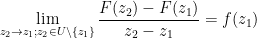
As it turns out, the fundamental theorem of calculus continues to hold in the complex plane: under suitable regularity assumptions on a complex function 
whenever 


— 1. Integration along a contour —
The notion of a curve is a very intuitive one. However, the precise mathematical definition of what a curve actually is depends a little bit on what type of mathematics one wishes to do. If one is mostly interested in topology, then a good notion is that of a continuous (parameterised) curve. If one wants to do analysis in somewhat irregular domains, it is convenient to restrict the notion of curve somewhat, to the rectifiable curves. If one is doing analysis in “nice” domains (such as the complex plane 
We begin by defining the notion of a continuous curve.
Definition 1 (Continuous curves) A continuous parameterised curve, or curve for short, is a continuous map
from a compact interval
to the complex plane
, and non-trivial otherwise. We refer to the complex numbers
as the initial point and terminal point (or final point) of the curve respectively, and refer to these two points collectively as the endpoints of the curve. We say that the curve is closed if
. We say that the curve is simple if one has
for any distinct
, with the possible exception of the endpoint cases
or
(thus we allow closed curves to be simple). We refer to the subset
of the complex plane as the image of the curve.
We caution that the term “closed” here does not refer to the topological notion of closure: for any curve ![{\gamma([a,b])}](https://s0.wp.com/latex.php?latex=%7B%5Cgamma%28%5Ba%2Cb%5D%29%7D&bg=ffffff&fg=000000&s=0&c=20201002)
A basic example of a curve is the directed line segment ![{\gamma_{z_1 \rightarrow z_2}: [0,1] \rightarrow {\bf C}}](https://s0.wp.com/latex.php?latex=%7B%5Cgamma_%7Bz_1+%5Crightarrow+z_2%7D%3A+%5B0%2C1%5D+%5Crightarrow+%7B%5Cbf+C%7D%7D&bg=ffffff&fg=000000&s=0&c=20201002)


for 


![{\gamma_{z_0,r,\circlearrowleft}: [0,2\pi] \rightarrow {\bf C}}](https://s0.wp.com/latex.php?latex=%7B%5Cgamma_%7Bz_0%2Cr%2C%5Ccirclearrowleft%7D%3A+%5B0%2C2%5Cpi%5D+%5Crightarrow+%7B%5Cbf+C%7D%7D&bg=ffffff&fg=000000&s=0&c=20201002)


This is a simple closed non-trivial curve. If we extended the domain here from ![{[0,2\pi]}](https://s0.wp.com/latex.php?latex=%7B%5B0%2C2%5Cpi%5D%7D&bg=ffffff&fg=000000&s=0&c=20201002)
![{[0,4\pi]}](https://s0.wp.com/latex.php?latex=%7B%5B0%2C4%5Cpi%5D%7D&bg=ffffff&fg=000000&s=0&c=20201002)
Note that it is technically possible for two distinct curves to have the same image. For instance, the anti-clockwise circle ![{\tilde \gamma_{z_0,r,\circlearrowleft}: [0,1] \rightarrow {\bf C}}](https://s0.wp.com/latex.php?latex=%7B%5Ctilde+%5Cgamma_%7Bz_0%2Cr%2C%5Ccirclearrowleft%7D%3A+%5B0%2C1%5D+%5Crightarrow+%7B%5Cbf+C%7D%7D&bg=ffffff&fg=000000&s=0&c=20201002)

traverses the same image as the previous curve (2), but is considered a distinct curve from 
![{\gamma_2: [a_2,b_2] \rightarrow {\bf C}}](https://s0.wp.com/latex.php?latex=%7B%5Cgamma_2%3A+%5Ba_2%2Cb_2%5D+%5Crightarrow+%7B%5Cbf+C%7D%7D&bg=ffffff&fg=000000&s=0&c=20201002)
![{\gamma_1: [a_1, b_1] \rightarrow {\bf C}}](https://s0.wp.com/latex.php?latex=%7B%5Cgamma_1%3A+%5Ba_1%2C+b_1%5D+%5Crightarrow+%7B%5Cbf+C%7D%7D&bg=ffffff&fg=000000&s=0&c=20201002)
![{\phi: [a_1,b_1] \rightarrow [a_2,b_2]}](https://s0.wp.com/latex.php?latex=%7B%5Cphi%3A+%5Ba_1%2Cb_1%5D+%5Crightarrow+%5Ba_2%2Cb_2%5D%7D&bg=ffffff&fg=000000&s=0&c=20201002)
![{\phi^{-1}: [a_2,b_2] \rightarrow [a_1,b_1]}](https://s0.wp.com/latex.php?latex=%7B%5Cphi%5E%7B-1%7D%3A+%5Ba_2%2Cb_2%5D+%5Crightarrow+%5Ba_1%2Cb_1%5D%7D&bg=ffffff&fg=000000&s=0&c=20201002)


![{t \in [a_1,b_1]}](https://s0.wp.com/latex.php?latex=%7Bt+%5Cin+%5Ba_1%2Cb_1%5D%7D&bg=ffffff&fg=000000&s=0&c=20201002)


Exercise 2 Let
- (i) Show that
is a homeomorphism. (Hint: use the fact that a continuous image of a compact set is compact, and that a subset of an interval is topologically closed if and only if it is compact.)
- (ii) If
and that
- (iii) Conversely, if
is a continuous monotone increasing map with
and
, show that
is a homeomorphism.
It will be important for us that we do not allow reparameterisations to reverse the endpoints. For instance, if 


![{[0,1]}](https://s0.wp.com/latex.php?latex=%7B%5B0%2C1%5D%7D&bg=ffffff&fg=000000&s=0&c=20201002)
![{-\gamma: [-b,-a] \rightarrow {\bf C}}](https://s0.wp.com/latex.php?latex=%7B-%5Cgamma%3A+%5B-b%2C-a%5D+%5Crightarrow+%7B%5Cbf+C%7D%7D&bg=ffffff&fg=000000&s=0&c=20201002)

Another basic operation on curves is that of concatenation. Suppose we have two curves ![{\gamma_1: [a_1,b_1] \rightarrow {\bf C}}](https://s0.wp.com/latex.php?latex=%7B%5Cgamma_1%3A+%5Ba_1%2Cb_1%5D+%5Crightarrow+%7B%5Cbf+C%7D%7D&bg=ffffff&fg=000000&s=0&c=20201002)


![{\tilde \gamma_2: [b_1, b_2+b_1-a_2] \rightarrow {\bf C}}](https://s0.wp.com/latex.php?latex=%7B%5Ctilde+%5Cgamma_2%3A+%5Bb_1%2C+b_2%2Bb_1-a_2%5D+%5Crightarrow+%7B%5Cbf+C%7D%7D&bg=ffffff&fg=000000&s=0&c=20201002)
![{\gamma_1 + \gamma_2: [a_1, b_2+b_1-a_2] \rightarrow {\bf C}}](https://s0.wp.com/latex.php?latex=%7B%5Cgamma_1+%2B+%5Cgamma_2%3A+%5Ba_1%2C+b_2%2Bb_1-a_2%5D+%5Crightarrow+%7B%5Cbf+C%7D%7D&bg=ffffff&fg=000000&s=0&c=20201002)

for 
for 


Concatenation is well behaved with respect to equivalence and reversal:
Exercise 3 Let
be continuous curves. Suppose that the terminal point of
.
- (i) (Concatenation and reversal well defined up to equivalence) If
and
, show that
and
.
- (ii) (Concatenation associative) Show that
. In particular, we certainly have

- (iii) (Concatenation and reversal) Show that
.
- (iv) (Non-commutativity) Give an example in which
are both well-defined, but not equivalent to each other.
- (v) (Identity) If
is the trivial curve
defined for any
, show that
and
.
- (vi) (Non-invertibility) Give an example in which
is not equivalent to a trivial curve. (It will however be homologous to a trivial curve, as we will discuss in later notes.)
Remark 4 The above exercise allows one to view the space of curves up to equivalence as a category, with the points in the complex plane being the objects of the category, and each equivalence class of curves being a single morphism from the initial point to the terminal point (and with the equivalence class of trivial curves being the identity morphisms). This point of view can be useful in topology, particularly when relating to concepts such as the fundamental group (and fundamental groupoid), monodromy, and holonomy. However, we will not need to use any advanced category-theoretic concepts in this course.
Exercise 5 Let
, let
denote the curve
(thus for instance
).
- (i) Show that for any integer
.
- (ii) Show that for any non-negative integers
, we have
. What happens for other values of
- (ii) If
.

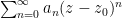
Given a sequence of complex numbers 


This is well-defined thanks to Exercise 3(ii) (actually all we really need in applications is being well-defined up to equivalence). Thus for instance 

In order to do analysis, we need to restrict our attention to those curves which are rectifiable:
Definition 6 Let
of the curve is defined to be the supremum of the quantities
where
ranges over the natural numbers and
ranges over the partitions of

The concept is best understood visually: a curve is rectifiable if there is some finite bound on the length of polygonal paths one can form while traversing the curve in order. From Exercise 2 we see that equivalent curves have the same arclength, so the concepts of arclength and rectifiability are well defined for curves that are only given up to continuous reparameterisation.
Exercise 7 Let
be curves, with the terminal point of
In particular,
are both individually rectifiable.

It is not immediately obvious that any reasonable curve (e.g. the line segments
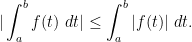
Lemma 8 (Triangle inequality) Let
be a continuous function. Then
Here we interpret
as the Riemann integral (or equivalently,
).
Proof: We first attempt to prove this inequality by considering the real and imaginary parts separately. From the real-valued triangle inequality (and basic properties of the Riemann integral) we have


and similarly

but these two bounds only yield the weaker estimate
To eliminate this 

But we have 


Exercise 9 Let
be real numbers. Show that the interval
is a non-empty set that is both open and closed in
such that
.)
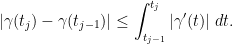
Next, we say that a non-trivial curve
![\displaystyle \gamma'(t) := \lim_{t' \rightarrow t: t' \in [a,b] \backslash \{t\}} \frac{\gamma(t') - \gamma(t)}{t'-t}](https://s0.wp.com/latex.php?latex=%5Cdisplaystyle++%5Cgamma%27%28t%29+%3A%3D+%5Clim_%7Bt%27+%5Crightarrow+t%3A+t%27+%5Cin+%5Ba%2Cb%5D+%5Cbackslash+%5C%7Bt%5C%7D%7D+%5Cfrac%7B%5Cgamma%28t%27%29+-+%5Cgamma%28t%29%7D%7Bt%27-t%7D&bg=ffffff&fg=000000&s=0&c=20201002)
exists and is continuous for all ![{t \in [a,b]}](https://s0.wp.com/latex.php?latex=%7Bt+%5Cin+%5Ba%2Cb%5D%7D&bg=ffffff&fg=000000&s=0&c=20201002)


Proposition 10 (Arclength formula) If

Proof: We first prove the upper bound
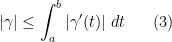
which in particular implies the rectifiability of 

for any 
Summing in 

and taking suprema over all partitions we obtain (3).
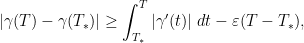
Now we need to show the matching lower bound. Let 

![{\gamma_{[a,T]}: [a,T] \rightarrow {\bf C}}](https://s0.wp.com/latex.php?latex=%7B%5Cgamma_%7B%5Ba%2CT%5D%7D%3A+%5Ba%2CT%5D+%5Crightarrow+%7B%5Cbf+C%7D%7D&bg=ffffff&fg=000000&s=0&c=20201002)
![{[a,T]}](https://s0.wp.com/latex.php?latex=%7B%5Ba%2CT%5D%7D&bg=ffffff&fg=000000&s=0&c=20201002)
![\displaystyle |\gamma_{[a,T]}| \geq \int_a^T |\gamma'(t)|\ dt - \varepsilon (T-a) \ \ \ \ \ (4)](https://s0.wp.com/latex.php?latex=%5Cdisplaystyle++%7C%5Cgamma_%7B%5Ba%2CT%5D%7D%7C+%5Cgeq+%5Cint_a%5ET+%7C%5Cgamma%27%28t%29%7C%5C+dt+-+%5Cvarepsilon+%28T-a%29+%5C+%5C+%5C+%5C+%5C+%284%29&bg=ffffff&fg=000000&s=0&c=20201002)
for all 

It remains to prove (4) for a given choice of 
Let ![{\Omega_\varepsilon \subset [a,b]}](https://s0.wp.com/latex.php?latex=%7B%5COmega_%5Cvarepsilon+%5Csubset+%5Ba%2Cb%5D%7D&bg=ffffff&fg=000000&s=0&c=20201002)

![{|\gamma_{[a,T]}|}](https://s0.wp.com/latex.php?latex=%7B%7C%5Cgamma_%7B%5Ba%2CT%5D%7D%7C%7D&bg=ffffff&fg=000000&s=0&c=20201002)


![{[T_*, T_*+\delta] \subset [a,b]}](https://s0.wp.com/latex.php?latex=%7B%5BT_%2A%2C+T_%2A%2B%5Cdelta%5D+%5Csubset+%5Ba%2Cb%5D%7D&bg=ffffff&fg=000000&s=0&c=20201002)

for all ![{T \in [T_*, T_*+\delta]}](https://s0.wp.com/latex.php?latex=%7BT+%5Cin+%5BT_%2A%2C+T_%2A%2B%5Cdelta%5D%7D&bg=ffffff&fg=000000&s=0&c=20201002)

Also, from the continuity of 

for all 
and hence
![\displaystyle |\gamma_{[T_*,T]}| \geq \int_{T_*}^T |\gamma'(t)|\ dt - \varepsilon (T-T_*)](https://s0.wp.com/latex.php?latex=%5Cdisplaystyle++%7C%5Cgamma_%7B%5BT_%2A%2CT%5D%7D%7C+%5Cgeq+%5Cint_%7BT_%2A%7D%5ET+%7C%5Cgamma%27%28t%29%7C%5C+dt+-+%5Cvarepsilon+%28T-T_%2A%29&bg=ffffff&fg=000000&s=0&c=20201002)
where ![{\gamma_{[T_*,T]}: [T_*,T] \rightarrow {\bf C}}](https://s0.wp.com/latex.php?latex=%7B%5Cgamma_%7B%5BT_%2A%2CT%5D%7D%3A+%5BT_%2A%2CT%5D+%5Crightarrow+%7B%5Cbf+C%7D%7D&bg=ffffff&fg=000000&s=0&c=20201002)
![{[T_*,T]}](https://s0.wp.com/latex.php?latex=%7B%5BT_%2A%2CT%5D%7D&bg=ffffff&fg=000000&s=0&c=20201002)

![{T \in [T_*,T_*+\delta]}](https://s0.wp.com/latex.php?latex=%7BT+%5Cin+%5BT_%2A%2CT_%2A%2B%5Cdelta%5D%7D&bg=ffffff&fg=000000&s=0&c=20201002)
![{\Omega_\varepsilon = [a,b]}](https://s0.wp.com/latex.php?latex=%7B%5COmega_%5Cvarepsilon+%3D+%5Ba%2Cb%5D%7D&bg=ffffff&fg=000000&s=0&c=20201002)
It is now easy to verify that the line segment 


Exercise 11 Show that the curve
defined by setting
for
and
is continuous but not rectifiable. (Hint: it is not necessary to compute the arclength precisely; a lower bound that goes to infinity will suffice. Graph the curve to discover some convenient partitions with which to generate such lower bounds. Alternatively, one can apply the arclength formula to some subcurves of
Exercise 12 (This exercise presumes familiarity with Lebesgue measure.) Show that the image of a rectifiable curve is necessarily of measure zero in the complex plane. (In particular, space-filling curves such as the Peano curve or the Hilbert curve cannot be rectifiable.)
Remark 13 As the above exercise suggests, many fractal curves will fail to be rectifiable; for instance the Koch snowflake is a famous example of an unrectifiable curve. (The situation is clarified once one develops the theory of Hausdorff dimension, as is done for instance in this previous post: any curve of Hausdorff dimension strictly greater than one will be unrectifiable.)
Exercise 14 (Arclength parameterisation) Let
- (i) Show that the arclength of the restriction of
for
varies continuously in
. (Hint: you may find it convenient to first establish the preliminary bound
for any
and
, and similarly
for any
.)
- (ii) Assume furthermore that
with the property that for each
, the restriction of
to
has arclength exactly
Much as continuous functions ![{f: \gamma([a,b]) \rightarrow {\bf C}}](https://s0.wp.com/latex.php?latex=%7Bf%3A+%5Cgamma%28%5Ba%2Cb%5D%29+%5Crightarrow+%7B%5Cbf+C%7D%7D&bg=ffffff&fg=000000&s=0&c=20201002)
Proposition 15 (Integration in rectifiable curves) Let
where
is an element of
, converge as the maximum mesh size
goes to zero to some complex limit, which we will denote as
such that
whenever
.


Proof: In real analysis courses, one often uses the order properties of the real line to replace the rather complicated looking Riemann sums with the simpler Darboux sums, en route to proving the real-variable analogue of the above proposition. However, in our complex setting the ordering of the real line is not available, so we will tackle the Riemann sums directly rather than try to compare them with Darboux sums.
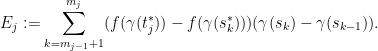
It suffices to prove that the “Riemann sums” (5) are a Cauchy sequence (or more precisely a Cauchy net), in the sense that the difference

between two sums of the form (5) is smaller than any specified 


where
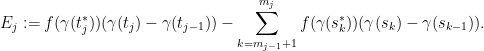
By telescoping series, we may rearrange 
As
for all 

and hence on summing in
Since
One cannot simply omit the rectifiability hypothesis from the above proposition:
Exercise 16 Give an example of a curve
fail to converge to a limit as the maximum mesh size goes to zero, so the integral
does not exist in the sense of convergent Riemann sums even though the integrand
near the origin. Come up with a variant of this curve which oscillates more. Nevertheless, it is still possible to assign a meaning to integrals such as
By abuse of notation, we will refer to the quantity
Exercise 17 Let
- (i) (Independence of parameterisation) If
is another curve equivalent to
.
- (ii) (Reversal) Show that
.
- (iii) (Concatenation) If
for some curves
- (iv) (Change of variables) If
- (v) (Upper bound) If there is a pointwise bound of the form
for all
and some
, show that
- (vi) (Linearity) If
is a complex number and
is a continuous function, show that
and
- (vii) (Integrating a constant) If
- (viii) (Uniform convergence) If
,
is a sequence of continuous functions converging uniformly to
, show that
converges to
- (ix) (Change of variables, II) Let
be an open neighbourhood of
be a holomorphic function, and let
be a continuous function. Show that
is rectifiable, and
(For this question, you may assume without proof that holomorphic functions are continuously differentiable; this fact will be proven (without reliance on this part of the exercise) in the next set of notes.)


Exercise 18 (This exercise assumes familiarity with the Riemann-Stieltjes integral.) Let
denote the monotone non-decreasing function
for
where the right-hand side is a Riemann-Stieltjes integral. Establish the triangle inequality
for any continuous
and obtain an alternate proof of Exercise 17(v).
![\displaystyle g(T) := |\gamma_{[a,T]}|](https://s0.wp.com/latex.php?latex=%5Cdisplaystyle++g%28T%29+%3A%3D+%7C%5Cgamma_%7B%5Ba%2CT%5D%7D%7C&bg=ffffff&fg=000000&s=0&c=20201002)

The change of variables formula (iv) lets one compute many contour integrals using the familiar Riemann integral. For instance, if 
and on reversal we also have

Similarly, if 

Remark 19 We caution that if
may introduce some non-trivial imaginary part, as is the case for instance in (6). For similar reasons, we have
and
in general. If one wishes to mix line integrals with real and imaginary parts, it is recommended to replace the contour integrals above with the line integrals
which are defined as in Proposition 15 but where the expression
appearing in (5) is replaced by
The contour integral corresponds to the special case
(or more informally,
). Line integrals are in turn special cases of the more general concept of integration of differential forms, discussed for instance in this article of mine, and which are used extensively in differential geometry and geometric topology. However we will not use these more general line integrals or differential form integrals much in this course.


In later notes it will be convenient to restrict to a more regular class of curves than the rectifiable curves. We thus give the definitions here:
Definition 20 (Smooth curves and contours) A smooth curve is a curve
for all
Example 21 The line segments
are smooth curves and hence contours. Polygonal paths are usually not smooth, but they are contours. Any sum of finitely many contours is again a contour, and the reversal of a contour is also a contour.
Note here that the term “smooth” differs somewhat here from the real-variable notion of smoothness, which is defined to be “infinitely differentiable”. Smooth curves are still only assumed to just be continuously differentiable; we do not assume that the second derivative of
The following examples and exercises may help explain why the non-vanishing condition
Example 22 (Cuspidal curve) Consider the curve
defined by
. Clearly
vanishes at the origin. Indeed, the image of the curve is
, which looks visibly non-smooth at the origin if one plots it, due to the presence of a cusp.
Example 23 (Absolute value function) Consider the curve
. This curve is certainly continuously differentiable, and in fact is four times continuously differentiable, but is not smooth because
vanishes at the origin. The image of this curve is
, which looks visibly non-smooth at the origin (in particular, there is no unique tangent line to this curve here).
Example 24 (Spiral) Consider the curve
for
, and
; but it is not a smooth curve because
vanishes. The image of
Exercise 25 (Local behaviour of smooth curves) Let
be an interior point of
. Let
be a phase of
, thus
for some
of the image of
looks like a rotated graph, in the sense that
for some interval
containing the origin, and some continuously differentiable function
with
. Furthermore, show that
as
as
and
. The real-variable inverse function theorem will also be helpful.)
![\displaystyle \gamma([a,b]) \cap D(\gamma(t_0),\varepsilon) = \{ \gamma(t_0) + e^{i\theta} ( s + i f(s) ): s \in I_\varepsilon \}](https://s0.wp.com/latex.php?latex=%5Cdisplaystyle++%5Cgamma%28%5Ba%2Cb%5D%29+%5Ccap+D%28%5Cgamma%28t_0%29%2C%5Cvarepsilon%29+%3D+%5C%7B+%5Cgamma%28t_0%29+%2B+e%5E%7Bi%5Ctheta%7D+%28+s+%2B+i+f%28s%29+%29%3A+s+%5Cin+I_%5Cvarepsilon+%5C%7D&bg=ffffff&fg=000000&s=0&c=20201002)
Exercise 26 Show that a curve
Exercise 27 Show that the cuspidal curve and absolute value curves in Examples 22, 23 are contours, but the curve in Exercise 24 is not.
— 2. The fundamental theorem of calculus —
Now we establish the complex analogues of the fundamental theorem of calculus. As in the real-variable case, there are two useful formulations of this theorem. Here is the first:
Theorem 28 (First fundamental theorem of calculus) Let
be a continuous function, and suppose that
, that is to say a holomorphic function with
for all
. Let

Proof: If
We again use the continuity method. Let
![\displaystyle |\int_{\gamma_{[a,T]}} f(z)\ dz - (F(\gamma(T)) - F(\gamma(a)))| \leq \varepsilon |\gamma_{[a,T]}| \ \ \ \ \ (7)](https://s0.wp.com/latex.php?latex=%5Cdisplaystyle++%7C%5Cint_%7B%5Cgamma_%7B%5Ba%2CT%5D%7D%7D+f%28z%29%5C+dz+-+%28F%28%5Cgamma%28T%29%29+-+F%28%5Cgamma%28a%29%29%29%7C+%5Cleq+%5Cvarepsilon+%7C%5Cgamma_%7B%5Ba%2CT%5D%7D%7C+%5C+%5C+%5C+%5C+%5C+%287%29&bg=ffffff&fg=000000&s=0&c=20201002)
for all
Let 

![{[T_*,T_*+\delta] \subset [a,b]}](https://s0.wp.com/latex.php?latex=%7B%5BT_%2A%2CT_%2A%2B%5Cdelta%5D+%5Csubset+%5Ba%2Cb%5D%7D&bg=ffffff&fg=000000&s=0&c=20201002)

 , and hence
 ![\displaystyle |F(\gamma(T)) - F(\gamma(T_*)) - f(\gamma(T_*)) (\gamma(T)-\gamma(T_*))| \leq \varepsilon/2 |\gamma_{[T_*,T]}| \ \ \ \ \ (8)](https://s0.wp.com/latex.php?latex=%5Cdisplaystyle++%7CF%28%5Cgamma%28T%29%29+-+F%28%5Cgamma%28T_%2A%29%29+-+f%28%5Cgamma%28T_%2A%29%29+%28%5Cgamma%28T%29-%5Cgamma%28T_%2A%29%29%7C+%5Cleq+%5Cvarepsilon%2F2+%7C%5Cgamma_%7B%5BT_%2A%2CT%5D%7D%7C+%5C+%5C+%5C+%5C+%5C+%288%29&bg=ffffff&fg=000000&s=0&c=20201002)
for any

for all ![{t \in [T_*, T_*+\delta]}](https://s0.wp.com/latex.php?latex=%7Bt+%5Cin+%5BT_%2A%2C+T_%2A%2B%5Cdelta%5D%7D&bg=ffffff&fg=000000&s=0&c=20201002)
![\displaystyle |\int_{\gamma_{[T_*,T]}} (f(z) - f(\gamma(T_*)))\ dz| \leq \frac{\varepsilon}{2} |\gamma_{[T_*, T]}|](https://s0.wp.com/latex.php?latex=%5Cdisplaystyle++%7C%5Cint_%7B%5Cgamma_%7B%5BT_%2A%2CT%5D%7D%7D+%28f%28z%29+-+f%28%5Cgamma%28T_%2A%29%29%29%5C+dz%7C+%5Cleq+%5Cfrac%7B%5Cvarepsilon%7D%7B2%7D+%7C%5Cgamma_%7B%5BT_%2A%2C+T%5D%7D%7C&bg=ffffff&fg=000000&s=0&c=20201002)
where
![\displaystyle |\int_{\gamma_{[T_*,T]}} f(z)\ dz - f(\gamma(T_*)) (\gamma(T)-\gamma(T_*))| \leq \frac{\varepsilon}{2} |\gamma_{[T_*, T]}|.](https://s0.wp.com/latex.php?latex=%5Cdisplaystyle++%7C%5Cint_%7B%5Cgamma_%7B%5BT_%2A%2CT%5D%7D%7D+f%28z%29%5C+dz+-+f%28%5Cgamma%28T_%2A%29%29+%28%5Cgamma%28T%29-%5Cgamma%28T_%2A%29%29%7C+%5Cleq+%5Cfrac%7B%5Cvarepsilon%7D%7B2%7D+%7C%5Cgamma_%7B%5BT_%2A%2C+T%5D%7D%7C.&bg=ffffff&fg=000000&s=0&c=20201002)
Combining this with (8) and the triangle inequality, we conclude that
![\displaystyle |\int_{\gamma_{[T_*,T]}} f(z)\ dz - (F(\gamma(T)) - F(\gamma(T_*)))| \leq \varepsilon |\gamma_{[T_*,T]}|](https://s0.wp.com/latex.php?latex=%5Cdisplaystyle++%7C%5Cint_%7B%5Cgamma_%7B%5BT_%2A%2CT%5D%7D%7D+f%28z%29%5C+dz+-+%28F%28%5Cgamma%28T%29%29+-+F%28%5Cgamma%28T_%2A%29%29%29%7C+%5Cleq+%5Cvarepsilon+%7C%5Cgamma_%7B%5BT_%2A%2CT%5D%7D%7C&bg=ffffff&fg=000000&s=0&c=20201002)
and on adding this to the
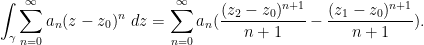
One can use this theorem to quickly evaluate many integrals by using an antiderivative for the integrand as in the real-variable case. For instance, for any rectifiable curve


and so forth. If the curve

since 


For the second fundamental theorem of calculus, we need a topological preliminary result.
Exercise 29 Let
- (i)
- (ii)
there exists a curve
- (iii)
(Hint: to show that (i) implies (iii), pick a base point
We remark that the relationship between path connectedness and connectedness is more delicate when one does not assume that the space
Remark 30 There is some debate as to whether to view the empty set
as connected, disconnected, or neither. I view this as analogous to the debate as to whether the natural number
In real analysis, the second fundamental theorem of calculus asserts that if a function 
Theorem 31 (Second fundamental theorem of calculus) Let
be a non-empty open connected subset of the complex numbers. Let
whenever
, and define the function
for all
, where
is any polygonal path from
follows from Exercise 17 and the conservative hypothesis (9)). Then
for all


Proof: We mimic the proof of the real-variable second fundamental theorem of calculus. Let 

and

and hence by Exercise 17

(The reader is strongly advised to draw a picture depicting the situation here.) Let 

for
for any
The notion of a non-empty open connected subset
The requirement that
Exercise 32 Let
- (i)
- (ii)
- (iii)
- (iv)
- (v)
(Hint: to show that (iii) implies (ii), induct on the number of edges in the closed polygonal path, and find a way to decompose non-simple closed polygonal paths into paths with fewer edges. One should avoid non-rigorous “hand-waving” arguments, and make sure that one actually has covered all possible cases, e.g. paths that include some backtracking.) Furthermore, show that if
, then there exists a constant
such that
.
Exercise 33 Show that the function
does not have an antiderivative on
.) In later notes we will see that
Exercise 34 If
Exercise 35 Let
- (i) Show that there is a unique collection
of non-empty subsets of
. (The elements of
- (ii) Show that the number of connected components of
- (iii) If
- (iv) If
).
Exercise 36 (Integration by parts) Let
be holomorphic functions on an open set

Note: the exercise below will be moved to a more logical location after the conclusion of the course.
Exercise 37 Let
be a curve. Show that the arclength
, where
is a partition of
whenever
there exists
whenever


103 comments
Comments feed for this article
21 October, 2020 at 1:30 pm
Anonymous
1.
One can identify what is going on here by rewriting the RHS:
2.
By the definition of , (4) follows. Recall that in order to prove the proposition, we want to prove (3) and (4).
25 October, 2020 at 8:02 am
Anonymous
Can a simple curve be equivalent to a non-simple curve up to continuous reparameterisation?
On the one hand, it seems yes by considering (2) with the domains![[0,2\pi]](https://s0.wp.com/latex.php?latex=%5B0%2C2%5Cpi%5D&bg=ffffff&fg=545454&s=0&c=20201002) and
and ![[0,4\pi]](https://s0.wp.com/latex.php?latex=%5B0%2C4%5Cpi%5D&bg=ffffff&fg=545454&s=0&c=20201002) , and the homomorphism
, and the homomorphism  between these two closed intervals. On the other hand, we don’t want (do we?) these two curves to be equivalent since they have different winding numbers. Am I missing something?
25 October, 2020 at 4:23 pm
Terence Tao
The reparameterisation of (2) using the change of variables is
is  ,
,  , which continues to wind around the origin exactly once.
25 October, 2020 at 4:38 pm
Anonymous
(Sorry for messing up the LaTeX code.)
I meant to ask that if the curve
![\displaystyle \gamma_1(\theta)=re^{i\theta},\quad \theta\in[0,2\pi]](https://s0.wp.com/latex.php?latex=%5Cdisplaystyle++%5Cgamma_1%28%5Ctheta%29%3Dre%5E%7Bi%5Ctheta%7D%2C%5Cquad+%5Ctheta%5Cin%5B0%2C2%5Cpi%5D++&bg=ffffff&fg=545454&s=0&c=20201002)
![\displaystyle \gamma_2(\theta)=re^{i\theta},\quad \theta\in[0,4\pi]](https://s0.wp.com/latex.php?latex=%5Cdisplaystyle++%5Cgamma_2%28%5Ctheta%29%3Dre%5E%7Bi%5Ctheta%7D%2C%5Cquad+%5Ctheta%5Cin%5B0%2C4%5Cpi%5D++&bg=ffffff&fg=545454&s=0&c=20201002)
and the curve
are equivalent up to continuous reparameterisation or not.
So the second one wind around the origin twice.
Is a reparameterisation of
  ?
?
[No. For instance, the arclengths are different. – T.]
25 October, 2020 at 5:25 pm
Anonymous
Ah, thanks. I confused myself with the definition. The homomorphism![\phi:[0,2\pi]\to[0,4\pi]](https://s0.wp.com/latex.php?latex=%5Cphi%3A%5B0%2C2%5Cpi%5D%5Cto%5B0%2C4%5Cpi%5D&bg=ffffff&fg=545454&s=0&c=20201002) with
with  would not work since
  .
.
25 October, 2020 at 2:12 pm
Anonymous
In the proof of Proposition 10,
… Adding this to the
I think “(7)” should be “Exercise 7”. Typo?
[Corrected, thanks – T.]
27 October, 2020 at 9:17 am
Wan-Teh Chang
Hi Prof. Tao,
I’d like to report some typos and suggest some minor edits in Notes 2.
In the sentence “We will explore this theorem and several of its consequences the next set of notes”, I suggest adding the word “in” before “the next set of notes”.
In Exercise 3 (i), “Concatenation well defined up to equivalence”, I suggest adding “and reversal” after “Concatenation”.
In Exercise 5 (i), “Show that for any integer “, remove “,
  “.
“.
In Definition 6, the subscripts in the summand are off by one. The subscripts in the summand should be and
and  , not
, not  and
and  .
.
At the end of the proof of Lemma 8 (Triangle inequality), “so taking the supremum of both sides in “, it suffices to take the supremum of the left-hand side because the right-hand side (a constant) is an upper bound of the left-hand side, and the supremum is
  any upper bound. Note: It also suffices to pick a particular value of
  to make the left-hand side a nonnegative real number.
In the proof of Proposition 10 (Arclength formula), “for any “, change
  to
to  .
.
In the proof of Proposition 10 (Arclength formula), in the inequality after “Summing in we obtain”, the indexes in the summand on the left-hand side should be
  and
and  , not
, not  and
and  .
.
In Proposition 14 (Integration in rectifiable curves), the last sentence “In other words, for every there exists a
  such that”, I suggest adding “
 ” after “
 .
.
In Exercise 26, “but the curve in Exercise 23 is not”, change “Exercise” to “Example”.
Optional: In the proof of Theorem 27 (First fundamental theorem of calculus), the variable is generally used to denote a number in the closed interval
 ![[T_{*}, T_{*} + \delta]](https://s0.wp.com/latex.php?latex=%5BT_%7B%2A%7D%2C+T_%7B%2A%7D+%2B+%5Cdelta%5D&bg=ffffff&fg=545454&s=0&c=20201002) . However, in the sentence “On the other hand, if
. However, in the sentence “On the other hand, if  is small enough, we have that …”, the variable
  is used instead (two occurrences). It would be good to use the variable
  consistently.
In the second-to-last sentence before Exercise 28, “…, and is a curve in
  with initial point
  and terminal point
  “, should we add “rectifiable” before “curve”?
In the hypothesis of Exercise 31, “Let be a non-empty connected subset of
  “, does
  ” need to be open?
In Exercise 34 (i), there is an uncommon symbol that looks like the set union operator with a sign inside. Is that a typo?
Thank you!
[Thanks for the corrections. I use in the proof of Theorem 27 to distinguish it from
  in the next line which will refer to a distinct time variable.
  is the symbol for disjoint union. -T]
23 November, 2020 at 2:47 pm
Anonymous
I recall that you called the “continuity method” some sort of induction.
One version of the continuous induction says the following:
If and
and
(1)
 then there exists
  such that
 then
then  .
.
(2) if
(3) if
Then .
.
Is the “continuity method” linked in this note the same as the notion of “continuous induction”?
26 November, 2020 at 11:33 am
Terence Tao
This is one instance of the continuity method (using the fact that the half-line is connected with respect to the right half-open topology). More generally, the continuity method can be applied to arbitrary connected topological spaces (not just the half-line); in particular in this course we frequently apply it to open connected subsets of the complex plane.
12 December, 2020 at 8:26 am
Anonymous
Is the continuity method related to (and can it be phrased as) transfinite induction?
12 December, 2020 at 11:22 am
Terence Tao
When one applies the continuity method to a totally ordered connected domain such as an interval, one can usually use transfinite induction (or Zorn’s lemma) as a substitute for the method. However the continuity method can also be applied to other connected domains (e.g., open connected subsets of the complex plane), for which it is less evident how to apply transfinite induction (though in many cases one could take advantage of path connectedness and apply transfinite induction along each path separately).
28 November, 2020 at 3:33 pm
Anonymous
If one considers continuous curves but only differentiable reparametrisations, would one loose anything?
28 November, 2020 at 4:38 pm
Anonymous
If![\gamma_1:[a_1,b_1]\to{\bf C}](https://s0.wp.com/latex.php?latex=%5Cgamma_1%3A%5Ba_1%2Cb_1%5D%5Cto%7B%5Cbf+C%7D&bg=ffffff&fg=545454&s=0&c=20201002) is equivalent to
is equivalent to ![\gamma_2:[a_2,b_2]\to{\bf C}](https://s0.wp.com/latex.php?latex=%5Cgamma_2%3A%5Ba_2%2Cb_2%5D%5Cto%7B%5Cbf+C%7D&bg=ffffff&fg=545454&s=0&c=20201002) up to continuous reparametrisation, i.e.,
up to continuous reparametrisation, i.e.,  for some endpoint preserving
  , is such
  unique? If not, can one always find a
  that is differentiable?
29 November, 2020 at 1:54 pm
Anonymous
It is not unique. One can always find one that is differentiable.
30 November, 2020 at 1:55 pm
Anonymous
Would it be circular somewhere if one uses Theorem 27 to prove Exercise 16(vii)?
[Probably, and in any event Theorem 27 is only applicable to holomorphic functions whereas Exercise 16 only requires continuity of the integrand. -T]
27 September, 2021 at 9:00 am
246A, Notes 1: complex differentiation | What's new
[…] Previous set of notes: Notes 0. Next set of notes: Notes 2. […]
8 April, 2022 at 7:44 am
J
… The contour integral can be viewed as the special case of the more general *line integral*
The linked Wikipedia article to “line integral” seems a bit confusing. In that article, “complex line integral” refers to the notion of “contour integrals” in this set of notes. On the other hand, they only define the line integral when
when  and
and  are both real-valued; that’s what they call the line integral for (real) vector fields. Any other references?
According to your PCM article on differential forms linked in this note, the Euclidean structure (dot product) is not needed in the integrals of differential forms, particularly the line integrals. Since the contour integral can be viewed as a special line integral, is it also “independent” of the metric structure of paths in the complex plane? But this would seem to contradict the discussion of rectifiable curves where a metric is needed.
10 April, 2022 at 8:53 pm
Terence Tao
One can define line integrals for complex simply by computing the real and imaginary parts of the integral separately, much as one can compute the Riemann integral of a complex function in terms of the Riemann integral of the real and imaginary parts.
Rectificability only needs the metric structure up to Lipschitz equivalence; the Euclidean metric can be replaced by any other Lipschitz equivalent metric and one still has the same notion of rectifiability. Because all norms on a finite dimensional vector space are equivalent, the notion of rectifiability thus does not require any specific metric structure on this space.
9 April, 2022 at 8:16 pm
Anonymous
[Corrected, thanks – T.]
24 April, 2022 at 5:01 am
N is a number
Professor Tao, you have mentioned the terms “signed definite integral” and “unsigned integral” quite a few times in different contexts, and here too you started by stating these while reviewing the notions of integration one has for a real-valued function![f: [ a,b] \to \mathbf{R}](https://s0.wp.com/latex.php?latex=f%3A+%5B+a%2Cb%5D+%5Cto+%5Cmathbf%7BR%7D&bg=ffffff&fg=545454&s=0&c=20201002) of one real variable.
of one real variable.
Could you please motivate these terms? What does it mean to call one of them as signed and the other as unsigned?
24 April, 2022 at 7:04 am
N is a number
OK, I realize that the terms are adopted to distinguish between the cases of assigning or not assigning an orientation to the region or domain of integration.
Is this the only reason?
25 April, 2022 at 11:46 am
Terence Tao
The unsigned integral![\int_{[a,b]} f(x)\ dx](https://s0.wp.com/latex.php?latex=%5Cint_%7B%5Ba%2Cb%5D%7D+f%28x%29%5C+dx&bg=ffffff&fg=545454&s=0&c=20201002) of an unsigned function
of an unsigned function  is still unsigned, but the signed integral
  of an unsigned function can be negative if
  .
.
29 May, 2022 at 12:32 am
Aditya Guha Roy
Exercise 12 can be solved by noticing that finite arc length implies inite 1-dimensional Hausdorff measure, which yields zero 2-dimensional Hausdorff measure.
Is there a more elementary proof without considering Hausdorff measures?
29 May, 2022 at 3:52 am
Aditya Guha Roy
(Minor correction) In Line number 10 in the proof of Proposition 10 (Arc-length formula) there is a mismatch of and
and  when you write
  while indexing the summands by
  .
.
[Corrected, thanks – T.]
29 May, 2022 at 4:09 am
Aditya Guha Roy
Also none of the tricki links are in working condition anymore. It says that the “site is offline”.
7 June, 2022 at 4:28 am
Cheng Yui To
For exercise 14, the reparametrization will not be continuous if the curve is constant on some interval right?
[Oops, this hypothesis needs to be added, thanks – T.]