Math 246A, Notes 3: Cauchy’s theorem and its consequences

2 October, 2016 in 246A - complex analysis, math.AT, math.CV | Tags: Cauchy's theorem, contour integration, Jordan's theorem, simply connected | by Terence Tao

Previous set of notes: Notes 2. Next set of notes: Notes 4.

We now come to perhaps the most central theorem in complex analysis (save possibly for the fundamental theorem of calculus), namely Cauchy’s theorem, which allows one to compute a large number of contour integrals ${\int_\gamma f(z)\ dz}$ even without knowing any explicit antiderivative of ${f}$ . There are many forms and variants of Cconauchy’s theorem. To give one such version, we need the basic topological notion of a homotopy:

Definition 1 (Homotopy) Let ${U}$ be an open subset of ${{\bf C}}$ , and let ${\gamma_0: [a,b] \rightarrow U}$ , ${\gamma_1: [a,b] \rightarrow U}$ be two curves in ${U}$ .

(i) If ${\gamma_0, \gamma_1}$ have the same initial point ${z_0}$ and terminal point ${z_1}$ , we say that ${\gamma_0}$ and ${\gamma_1}$ are homotopic with fixed endpoints in ${U}$ if there exists a continuous map ${\gamma: [0,1] \times [a,b] \rightarrow U}$ such that ${\gamma(0,t) = \gamma_0(t)}$ and ${\gamma(1,t) = \gamma_1(t)}$ for all ${t \in [a,b]}$ , and such that ${\gamma(s,a) = z_0}$ and ${\gamma(s,b) = z_1}$ for all ${s \in [0,1]}$ .

(ii) If ${\gamma_0, \gamma_1}$ are closed (but possibly with different initial points), we say that ${\gamma_0}$ and ${\gamma_1}$ are homotopic as closed curves in ${U}$ if there exists a continuous map ${\gamma: [0,1] \times [a,b] \rightarrow U}$ such that ${\gamma(0,t) = \gamma_0(t)}$ and ${\gamma(1,t) = \gamma_1(t)}$ for all ${t \in [a,b]}$ , and such that ${\gamma(s,a) = \gamma(s,b)}$ for all ${s \in [0,1]}$ .

(iii) If ${\gamma_2: [c,d] \rightarrow U}$ and ${\gamma_3: [e,f] \rightarrow U}$ are curves with the same initial point and same terminal point, we say that ${\gamma_2}$ and ${\gamma_3}$ are homotopic with fixed endpoints up to reparameterisation in ${U}$ if there is a reparameterisation ${\tilde \gamma_2: [a,b] \rightarrow U}$ of ${\gamma_2}$ which is homotopic with fixed endpoints in ${U}$ to a reparameterisation ${\tilde \gamma_3: [a,b] \rightarrow U}$ of ${\gamma_3}$ .

(iv) If ${\gamma_2: [c,d] \rightarrow U}$ and ${\gamma_3: [e,f] \rightarrow U}$ are closed curves, we say that ${\gamma_2}$ and ${\gamma_3}$ are homotopic as closed curves up to reparameterisation in ${U}$ if there is a reparameterisation ${\tilde \gamma_2: [a,b] \rightarrow U}$ of ${\gamma_2}$ which is homotopic as closed curves in ${U}$ to a reparameterisation ${\tilde \gamma_3: [a,b] \rightarrow U}$ of ${\gamma_3}$ .

In the first two cases, the map ${\gamma}$ will be referred to as a homotopy from ${\gamma_0}$ to ${\gamma_1}$ , and we will also say that ${\gamma_0}$ can be continously deformed to ${\gamma_1}$ (either with fixed endpoints, or as closed curves).

Example 2 If ${U}$ is a convex set, that is to say that ${(1-s) z_0 + s z_1 \in U}$ whenever ${z_0,z_1 \in U}$ and ${0 \leq s \leq 1}$ , then any two curves ${\gamma_0, \gamma_1: [0,1] \rightarrow U}$ from one point ${z_0}$ to another ${z_1}$ are homotopic, by using the homotopy

$\displaystyle \gamma(s,t) := (1-s) \gamma_0(t) + s \gamma_1(t).$

For a similar reason, in a convex open set ${U}$ , any two closed curves will be homotopic to each other as closed curves.

Exercise 3 Let ${U}$ be an open subset of ${{\bf C}}$ .

(i) Prove that the property of being homotopic with fixed endpoints in ${U}$ is an equivalence relation.

(ii) Prove that the property of being homotopic as closed curves in ${U}$ is an equivalence relation.

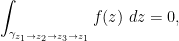
(iii) If ${\gamma_0: [a,b] \rightarrow U}$ , ${\gamma_1: [c,d] \rightarrow U}$ are closed curves with the same initial point, show that ${\gamma_0}$ is homotopic to ${\gamma_1}$ as closed curves up to reparameterisation if and only if ${\gamma_0}$ is homotopic to ${\gamma_2 + \gamma_1 + (-\gamma_2)}$ with fixed endpoints for some closed curve ${\gamma_2}$ with the same initial point as ${\gamma_0}$ or ${\gamma_1}$ up to reparameterisation. (Hint: it may be conceptually easier to think about the case when ${\gamma_0, \gamma_1}$ do not necessarily have the same initial point, in which case the same claim is true, except that ${\gamma_2}$ is now not a closed curve, but rather a curve that starts at the initial point of ${\gamma_0}$ and ends at the initial point of ${\gamma_1}$ .) For an additional challenge: propose a counterexample that explains why the curve ${\gamma_2}$ is necessary (in the initial context where ${\gamma_0}$ , ${\gamma_1}$ have the same initial point).

(iv) Define a point in ${U}$ to be a curve ${\gamma_1: [a,b] \rightarrow U}$ of the form ${\gamma_1(t) = z_0}$ for some ${z_0 \in U}$ and all ${t \in [a,b]}$ . Let ${\gamma_0: [a,b] \rightarrow U}$ be a closed curve in ${U}$ . Show that ${\gamma_0}$ is homotopic with fixed endpoints to a point in ${U}$ if and only if ${\gamma_0}$ is homotopic as a closed curve to a point in ${U}$ . (In either case, we will call ${\gamma_0}$ homotopic to a point, null-homotopic, or contractible to a point in ${U}$ .)

(v) If ${\gamma_0, \gamma_1: [a,b] \rightarrow U}$ are curves with the same initial point and the same terminal point, show that ${\gamma_0}$ is homotopic to ${\gamma_1}$ with fixed endpoints in ${U}$ if and only if ${\gamma_0 + (-\gamma_1)}$ is homotopic to a point in ${U}$ .

(vi) If ${U}$ is connected, and ${\gamma_0, \gamma_1: [a,b] \rightarrow U}$ are any two curves in ${U}$ , show that there exists a continuous map ${\gamma: [0,1] \times [a,b] \rightarrow U}$ such that ${\gamma(0,t) = \gamma_0(t)}$ and ${\gamma(1,t) = \gamma_1(t)}$ for all ${t \in [a,b]}$ . Thus the notion of homotopy becomes rather trivial if one does not fix the endpoints or require the curve to be closed.

(vii) Show that if ${\gamma_1: [a,b] \rightarrow U}$ is a reparameterisation of ${\gamma_0: [a,b] \rightarrow U}$ , then ${\gamma_0}$ and ${\gamma_1}$ are homotopic with fixed endpoints in U.

(viii) Prove that the property of being homotopic with fixed endpoints in ${U}$ up to reparameterisation is an equivalence relation.

(ix) Prove that the property of being homotopic as closed curves in ${U}$ up to reparameterisation is an equivalence relation.

We can then phrase Cauchy’s theorem as an assertion that contour integration on holomorphic functions is a homotopy invariant. More precisely:

Theorem 4 (Cauchy’s theorem) Let ${U}$ be an open subset of ${{\bf C}}$ , and let ${f: U \rightarrow {\bf C}}$ be holomorphic.

(i) If ${\gamma_0: [a,b] \rightarrow U}$ and ${\gamma_1: [c,d] \rightarrow U}$ are rectifiable curves that are homotopic in ${U}$ with fixed endpoints up to reparameterisation, then
$\displaystyle \int_{\gamma_0} f(z)\ dz = \int_{\gamma_1} f(z)\ dz.$

(ii) If ${\gamma_0: [a,b] \rightarrow U}$ and ${\gamma_1: [c,d] \rightarrow U}$ are closed rectifiable curves that are homotopic in ${U}$ as closed curves up to reparameterisation, then
$\displaystyle \int_{\gamma_0} f(z)\ dz = \int_{\gamma_1} f(z)\ dz.$

This version of Cauchy’s theorem is particularly useful for applications, as it explicitly brings into play the powerful technique of contour shifting, which allows one to compute a contour integral by replacing the contour with a homotopic contour on which the integral is easier to either compute or integrate. This formulation of Cauchy’s theorem also highlights the close relationship between contour integrals and the algebraic topology of the complex plane (and open subsets ${U}$ thereof). Setting ${\gamma_1}$ to be a point, we obtain an important special case of Cauchy’s theorem (which is in fact equivalent to the full theorem):

Corollary 5 (Cauchy’s theorem, again) Let ${U}$ be an open subset of ${{\bf C}}$ , and let ${f: U \rightarrow {\bf C}}$ be holomorphic. Then for any closed rectifiable curve ${\gamma}$ in ${U}$ that is contractible in ${U}$ to a point, one has ${\int_\gamma f(z)\ dz = 0}$ .

Exercise 6 Show that Theorem 4 and Corollary 5 are logically equivalent.

An important feature to note about Cauchy’s theorem is the global nature of its hypothesis on ${f}$ . The conclusion of Cauchy’s theorem only involves the values of a function ${f}$ on the images of the two curves ${\gamma_0, \gamma_1}$ . However, in order for the hypotheses of Cauchy’s theorem to apply, the function ${f}$ must be holomorphic not only on the images on ${\gamma_0, \gamma_1}$ , but on an open set ${U}$ that is large enough (and sufficiently free of “holes”) to support a homotopy between the two curves. This point can be emphasised through the following fundamental near-counterexample to Cauchy’s theorem:

Example 7 (Key example) Let ${U := {\bf C} \backslash \{0\}}$ , and let ${f: U \rightarrow {\bf C}}$ be the holomorphic function ${f(z) := \frac{1}{z}}$ . Let ${\gamma_{0,1,\circlearrowleft}: [0,2\pi] \rightarrow {\bf C}}$ be the closed unit circle contour ${\gamma_{0,1,\circlearrowleft}(t) := e^{it}}$ . Direct calculation shows that

$\displaystyle \int_{\gamma_{0,1,\circlearrowleft}} f(z)\ dz = 2\pi i \neq 0.$

As a consequence of this and Cauchy’s theorem, we conclude that the contour ${\gamma_{0,1,\circlearrowleft}}$ is not contractible to a point in ${U}$ ; note that this does not contradict Example 2 because ${U}$ is not convex. Thus we see that the lack of holomorphicity (or singularity) of ${f}$ at the origin can be “blamed” for the non-vanishing of the integral of ${f}$ on the closed contour ${\gamma_{0,1,\circlearrowleft}}$ , even though this contour does not come anywhere near the origin. Thus we see that the global behaviour of ${f}$ , not just the behaviour in the local neighbourhood of ${\gamma_{0,1,\circlearrowleft}}$ , has an impact on the contour integral.
One can of course rewrite this example to involve non-closed contours instead of closed ones. For instance, if we let ${\gamma_0, \gamma_1: [0,\pi] \rightarrow U}$ denote the half-circle contours ${\gamma_0(t) := e^{it}}$ and ${\gamma_1(t) := e^{-it}}$ , then ${\gamma_0,\gamma_1}$ are both contours in ${U}$ from ${+1}$ to ${-1}$ , but one has

$\displaystyle \int_{\gamma_0} f(z)\ dz = +\pi i$

whereas

$\displaystyle \int_{\gamma_1} f(z)\ dz = -\pi i.$

In order for this to be consistent with Cauchy’s theorem, we conclude that ${\gamma_0}$ and ${\gamma_1}$ are not homotopic in ${U}$ (even after reparameterisation).

In the specific case of functions of the form ${\frac{1}{z}}$ , or more generally ${\frac{f(z)}{z-z_0}}$ for some point ${z_0}$ and some ${f}$ that is holomorphic in some neighbourhood of ${z_0}$ , we can quantify the precise failure of Cauchy’s theorem through the Cauchy integral formula, and through the concept of a winding number. These turn out to be extremely powerful tools for understanding both the nature of holomorphic functions and the topology of open subsets of the complex plane, as we shall see in this and later notes.

— 1. Proof of Cauchy’s theorem —

The underlying reason for the truth of Cauchy’s theorem can be explained in one sentence: complex differentiable functions behave locally like complex linear functions, which are conservative thanks to the fundamental theorem of calculus. More precisely, if ${f(z) = a + bz}$ is any complex linear function of ${z}$ , then ${f}$ has an antiderivative ${az + \frac{1}{2} bz^2}$ , and hence

$\displaystyle \int_\gamma (a+bz)\ dz = 0 \ \ \ \ \ (1)$

for any rectifiable closed curve ${\gamma}$ in the complex plane.
Perhaps the slickest way to make this intuition rigorous is through the following special case of Cauchy’s theorem.

Theorem 8 (Goursat’s theorem) Let ${U}$ be an open subset of ${{\bf C}}$ , and ${z_1,z_2,z_3}$ be complex numbers such that the solid (and closed) triangle spanned by ${z_1,z_2,z_3}$ (or more precisely, the convex hull of ${\{z_1,z_2,z_3\}}$ ) is contained in ${U}$ . (We allow the triangle to degenerate in that we allow the ${z_1,z_2,z_3}$ to be collinear, or even coincident.) Then for any holomorphic function ${f: U \rightarrow {\bf C}}$ , one has

$\displaystyle \int_{\gamma_{z_1 \rightarrow z_2 \rightarrow z_3 \rightarrow z_1}} f(z)\ dz = 0,$

where ${\gamma_{z_1 \rightarrow z_2 \rightarrow z_3 \rightarrow z_1}}$ is the closed polygonal path that traverses the vertices ${z_1, z_2, z_3}$ of the solid triangle in order.

Proof: Let us denote the triangular contour ${\gamma_{z_1 \rightarrow z_2 \rightarrow z_3 \rightarrow z_1}}$ as ${T_0}$ . It is convenient (though odd-looking at first sight) to prove this theorem by contradiction. That is to say, suppose for contradiction that we had

$\displaystyle |\int_{T_0} f(z)\ dz| \geq \varepsilon \ \ \ \ \ (2)$

for some ${\varepsilon > 0}$ . We now run the following “divide and conquer” strategy. We let ${z_{12} := \frac{z_1+z_2}{2}}$ , ${z_{23} := \frac{z_2+z_3}{2}}$ , ${z_{31} := \frac{z_3 + z_1}{2}}$ be the midpoints of ${z_1, z_2, z_3}$ . Then from the basic properties of contour integration (see Exercise 17 of Notes 2) we can split the triangular integral ${\int_{T_1} f(z)\ dz}$ as the sum of four integrals on smaller triangles, namely

$\displaystyle \int_{\gamma_{z_1 \rightarrow z_{12} \rightarrow z_{31} \rightarrow z_1}} f(z)\ dz$

$\displaystyle \int_{\gamma_{z_{12} \rightarrow z_2 \rightarrow z_{23} \rightarrow z_{12}}} f(z)\ dz$

$\displaystyle \int_{\gamma_{z_{23} \rightarrow z_3 \rightarrow z_{31} \rightarrow z_{23}}} f(z)\ dz$

$\displaystyle \int_{\gamma_{z_{12} \rightarrow z_{23} \rightarrow z_{31} \rightarrow z_{12}}} f(z)\ dz.$

(The reader is encouraged to draw a picture to visualise this decomposition.) By (2) and the triangle inequality (or, if one prefers, the pigeonhole principle), we must therefore have

$\displaystyle |\int_{T_1} f(z)\ dz| \geq \frac{\varepsilon}{4}$

where ${T_1}$ is one of the four triangular contours ${\gamma_{z_1 \rightarrow z_{12} \rightarrow z_{31} \rightarrow z_1}}$ , ${\gamma_{z_{12} \rightarrow z_2 \rightarrow z_{23} \rightarrow z_{12}}}$ , ${\gamma_{z_{23} \rightarrow z_3 \rightarrow z_{31} \rightarrow z_{23}}}$ , or ${\gamma_{z_{12} \rightarrow z_{23} \rightarrow z_{31} \rightarrow z_{12}}}$ . Regardless of which of the four contours ${T_1}$ is, observe that the triangular region enclosed by ${T_1}$ is contained in that of ${T_0}$ . Furthermore, the diameter of ${T_1}$ is precisely half that of ${T_0}$ , where the diameter ${\mathrm{diam}(\gamma)}$ of a curve ${\gamma: [a,b] \rightarrow {\bf C}}$ is defined by the formula

$\displaystyle \mathrm{diam}(\gamma) := \sup_{t, t' \in [a,b]} |\gamma(t) - \gamma(t')|;$

similarly, the perimeter ${|T_1|}$ of ${T_1}$ is precisely half that of ${T_0}$ . If we iterate the above process, we can find a nested sequence ${T_0, T_1, T_2, \dots}$ of triangular contours, each of which is contained in the previous one with half the diameter and perimeter, such that

$\displaystyle |\int_{T_n} f(z)\ dz| \geq \frac{\varepsilon}{4^n} \ \ \ \ \ (3)$

for all ${n=0,1,2,\dots}$ . If we let ${z_n}$ be any point enclosed by ${T_n}$ , then from the decreasing diameters it is clear that the ${z_n}$ are a Cauchy sequence and thus converge to some limit ${z_*}$ , which is then contained in all of the closed triangles enclosed by any of the ${T_n}$ .
In particular, ${z_*}$ lies in ${U}$ and so ${f}$ is differentiable at ${z_*}$ . This implies, for any ${\varepsilon'>0}$ , that there exists a ${\delta > 0}$ such that

$\displaystyle |\frac{f(z) - f(z_*)}{z-z_*} - f'(z_*)| \leq \varepsilon'$

whenever ${z \in D(z_*,\delta) \backslash \{z_*\}}$ . We can rearrange this as

$\displaystyle |f(z) - (f(z_*) + (z-z_*) f'(z_*))| \leq \varepsilon' |z-z_*|$

on ${D(z_*,\delta)}$ . In particular, for ${n}$ large enough, this bound holds on the image on ${T_n}$ . In this case we can bound ${|z-z_*|}$ by ${\mathrm{diam}(T_n)}$ , and hence by Exercise 17(v) of Notes 2,

$\displaystyle |\int_{T_n} f(z)\ dz - \int_{T_n} (f(z_*) + (z-z_*) f'(z_*))\ dz| \leq \varepsilon' \hbox{diam}(T_n) |T_n|.$

From (1), the second integral vanishes. As each ${T_n}$ has half the diameter and perimeter of the previous, we thus have

$\displaystyle |\int_{T_n} f(z)\ dz| \leq \frac{\varepsilon' \hbox{diam}(T_0) |T_0|}{4^n}.$

But if one chooses ${\varepsilon'}$ small enough depending on ${\varepsilon}$ and ${T_0}$ , we contradict (3). $\Box$

Remark 9 This is a rare example of an argument in which a hypothesis of differentiability, rather than continuous differentiability, is used, because one can localise any failure of the conclusion all the way down to a single point. Another instance of such an argument is the standard proof of Rolle’s theorem.

Exercise 10 Find a proof of Goursat’s theorem that avoids explicit use of proof by contradiction. (Hint: use the fact that a solid triangle is compact, in the sense that every open cover has a finite subcover. For the purposes of this question, ignore the possibility that the proof of this latter fact might also use proof by contradiction.)

Goursat’s theorem only directly handles triangular contours, but as long as one works “locally”, or more precisely in a convex domain, we can quickly generalise:

Corollary 11 (Local Cauchy’s theorem for polygonal paths) Let ${U}$ be a convex open subset of ${{\bf C}}$ , and let ${f: U \rightarrow {\bf C}}$ be a holomorphic function. Then for any closed polygonal path ${\gamma = \gamma_{z_1 \rightarrow \dots \rightarrow z_n \rightarrow z_1}}$ in ${U}$ , we have ${\int_\gamma f(z)\ dz = 0}$ .

Proof: We induct on the number of vertices ${n}$ . The cases ${n=1,2}$ are trivial, and the ${n=3}$ case follows directly from Goursat’s theorem (using the convexity of ${U}$ to ensure that the interior of the polygon lies in ${U}$ ). If ${n > 3}$ , we can split

$\displaystyle \int_{\gamma_{z_1 \rightarrow \dots \rightarrow z_n \rightarrow z_1}} f(z)\ dz = \int_{\gamma_{z_1 \rightarrow \dots \rightarrow z_{n-1} \rightarrow z_1}} f(z)\ dz + \int_{z_{n-1} \rightarrow z_n \rightarrow z_1 \rightarrow z_{n-1}} f(z)\ dz.$

The second integral on the right-hand side vanishes by Goursat’s theorem. The claim then follows from induction. $\Box$

Exercise 12 By using the (real-variable) fundamental theorem of calculus and Fubini’s theorem in place of Goursat’s theorem, give an alternate proof of Corollary 11 in the case that ${\gamma}$ is a rectangle ${\gamma = \gamma_{a+bi \rightarrow c+bi \rightarrow c+di \rightarrow a+di \rightarrow a+bi}}$ and the derivative ${f'}$ of ${f}$ is continuous. (One can also use Stokes’ theorem in place of the fundamental theorem of calculus and Fubini’s theorem.)

We can amplify Corollary 11 using the fundamental theorem of calculus again:

Corollary 13 (Local Cauchy’s theorem) Let ${U}$ be a convex open subset of ${{\bf C}}$ , and let ${f: U \rightarrow {\bf C}}$ be a holomorphic function. Then ${f}$ has an antiderivative ${F: U \rightarrow {\bf C}}$ . Also, ${\int_\gamma f(z)\ dz = 0}$ for any closed rectifiable curve ${\gamma}$ in ${U}$ , and ${\int_{\gamma_1} f(z)\ dz = \int_{\gamma_2} f(z)\ dz}$ whenever ${\gamma_1, \gamma_2}$ are two rectifiable curves in ${U}$ with the same initial point and same terminal point. In other words, ${f}$ is conservative on ${U}$ .

Proof: The first claim follows from Corollary 11 and the second fundamental theorem of calculus (Theorem 31 from Notes 2). The remaining claims then follow from the first fundamental theorem of calculus (Theorem 28 from Notes 2). $\Box$

We can now prove Cauchy’s theorem in the form of Theorem 4.

Proof: We will just prove part (i), as part (ii) is similar (and in any event it follows from part (i)). Since reparameterisation does not affect the integral, we may assume without loss of generality that ${\gamma_0: [a,b] \rightarrow U}$ and ${\gamma_1: [a,b] \rightarrow U}$ are homotopic with fixed endpoints, and not merely homotopic with fixed endpoints up to reparameterisation.

Let ${\gamma: [0,1] \times [a,b] \rightarrow U}$ be a homotopy from ${\gamma_0}$ to ${\gamma_1}$ . Note that for any ${s \in [0,1]}$ and ${t \in [a,b]}$ , ${\gamma(s,t)}$ lies in the open set ${U}$ . From compactness, there must exist a radius ${r>0}$ such that ${D(\gamma(s,t),r) \subset U}$ for all ${s \in [0,1]}$ and ${t \in [a,b]}$ . Next, as ${\gamma}$ is continuous on a compact set, it is uniformly continuous. In particular, there exists ${\delta > 0}$ such that

$\displaystyle |\gamma(s',t') - \gamma(s,t)| \leq \frac{r}{4}$

whenever ${s,s' \in [0,1]}$ and ${t,t' \in [a,b]}$ are such that ${|s-s'| \leq \delta}$ and ${|t-t'| \leq \delta}$ .
Now partition ${[0,1]}$ and ${[a,b]}$ as ${0 = s_0 < \dots < s_n = 1}$ and ${a = t_0 < \dots < t_m = b}$ in such a way that ${|s_i - s_{i-1}| \leq \delta}$ and ${|t_j-t_{j-1}| \leq \delta}$ for all ${1 \leq i \leq n}$ and ${1 \leq j \leq m}$ . For each such ${i}$ and ${j}$ , let ${C_{i,j}}$ denote the closed polygonal contour

$\displaystyle C_{i,j} := \gamma_{\gamma(s_i,t_{j-1}) \rightarrow \gamma(s_i,t_j) \rightarrow \gamma(s_{i-1},t_j) \rightarrow \gamma(s_{i-1},t_{j-1}) \rightarrow \gamma(s_i,t_{j-1})}.$

(the reader is encouraged here to draw a picture of the situation; we are using polygonal contours here rather than the homotopy ${\gamma}$ because we did not require any rectifiability properties on the homotopy). By construction, the diameter of this contour is at most ${\frac{r}{4}+\frac{r}{4}+\frac{r}{4}+\frac{r}{4} = r}$ , so the contour is contained entirely in the disk ${D( \gamma(s_i,t_i), r)}$ . This disk is convex and contained in ${U}$ . Applying Corollary 11 or Corollary 13, we conclude that

$\displaystyle \int_{C_{i,j}} f(z)\ dz = 0$

for all ${1 \leq i \leq n}$ and ${1 \leq j \leq m}$ . If we sum this over all ${i}$ and ${j}$ , and noting that the homotopy fixes the endpoints, we conclude after a lot of cancelling that

$\displaystyle \int_{\gamma_{\gamma(0,t_0) \rightarrow \gamma(0, t_1) \rightarrow \dots \rightarrow \gamma(0, t_n)}} f(z)\ dz = \int_{\gamma_{\gamma(1,t_0) \rightarrow \gamma(1, t_1) \rightarrow \dots \rightarrow \gamma(1, t_n)}} f(z)\ dz$

(again, the reader is encouraged to draw a picture to see this cancellation). However, from a further application of Corollary 13 we have

$\displaystyle \int_{\gamma_{\gamma(0,t_{i-1}) \rightarrow \gamma(0,t_i)}} f(z)\ dz = \int_{\gamma_{0,[t_{i-1},t_i]}} f(z)\ dz$

for ${i=1,\dots,n}$ , where ${\gamma_{0,[t_{i-1},t_i]}: [t_{i-1},t_i] \rightarrow U}$ is the restriction of ${\gamma_0: [a,b] \rightarrow U}$ to ${[t_{i-1},t_i]}$ , and similarly for ${\gamma_1}$ . Putting all this together we conclude that

$\displaystyle \int_{\gamma_0} f(z)\ dz = \int_{\gamma_1} f(z)\ dz$

as required. $\Box$
One nice feature of Cauchy’s theorem is that it allows one to integrate holomorphic functions on curves that are not necessarily rectifiable. Indeed, if ${\gamma: [a,b] \rightarrow U}$ is a curve in ${U}$ , then for a sufficiently fine partition ${a = t_0 < t_1 < \dots < t_n = b}$ , the polygonal (and hence rectifiable) path ${\gamma_{t_0 \rightarrow t_1 \rightarrow \dots \rightarrow t_n}}$ will be contained in ${U}$ , and furthermore be homotopic to ${\gamma}$ with fixed endpoints. One can then define ${\int_\gamma f(z)\ dz}$ when ${f}$ is holomorphic in ${U}$ and ${\gamma}$ is non-rectifiable by declaring

$\displaystyle \int_\gamma f(z)\ dz := \int_{\tilde \gamma} f(z)\ dz$

where ${\tilde \gamma}$ is any rectifiable curve that is homotopic (with fixed endpoints) to ${\gamma}$ . This is a well defined definition thanks to the above discussion as well as Cauchy’s theorem; also observe that the exact open set ${U}$ in which the homotopy lives is not relevant, since given any two open sets ${U,U'}$ containing the image of ${\gamma}$ one can find a rectifiable curve ${\tilde \gamma}$ which is homotopic to ${\gamma}$ with fixed endpoints in ${U \cap U'}$ , and hence in ${U}$ and ${U'}$ separately. With this extended notion of the contour integral, one can then remove the hypothesis of rectifiability from many theorems involving integration of holomorphic functions. In particular, Cauchy’s theorem itself now holds for non-rectifiable curves. This reflects some duality in the integration concept ${\int_\gamma f(z)\ dz}$ ; if one assumes more regularity on the function ${f}$ , one can get away with worse regularity on the curve ${\gamma}$ , and vice versa.
A special case of Cauchy’s theorem is worth recording explicitly. We say that an open set ${U}$ in the complex plane is simply connected if it is non-empty, connected, and if every closed curve in ${U}$ is contractible in ${U}$ to a point. For instance, from Example 2 we see that any convex non-empty open set is simply connected. From Theorem 4 we then have

Theorem 14 (Cauchy’s theorem, simply connected case) Let ${U}$ be a simply connected subset of ${{\bf C}}$ , and let ${f: U \rightarrow {\bf C}}$ be holomorphic. Then ${\int_\gamma f(z)\ dz = 0}$ for any closed curve in ${U}$ . In particular (by Exercise 32 of Notes 2), ${f}$ is conservative and has an antiderivative.

One can interpret Cauchy’s theorem through the lens of algebraic topology, and particularly through the machinery of homology and cohomology. We will not develop this perspective in depth in these notes, but the following exercise will give a brief glimpse of the connections to homology and cohomology.

Exercise 15 Let ${U}$ be an open subset of ${{\bf C}}$ . Define a ${0}$ -chain in ${U}$ to be a formal linear combination

$\displaystyle \sum_{i=1}^n m_i [z_i]$

of points ${z_i \in U}$ (which we enclose in brackets to avoid confusion with the arithmetic operations on ${{\bf C}}$ , in particular ${[z]+[w]}$ is not identified with ${[z+w]}$ ), where ${n}$ is a natural number and the ${m_i}$ are integers; these form an additive abelian group in the usual fashion. Similarly, define a ${1}$ -chain in ${U}$ to be a formal linear combination

$\displaystyle \sum_{i=1}^n m_i [\gamma_i]$

of curves ${\gamma_i: [0,1] \rightarrow U}$ in ${U}$ , which (for very minor notational reasons) we will fix to have domain in the unit interval ${[0,1]}$ . Finally, define a ${2}$ -chain in ${U}$ to be a formal linear combination

$\displaystyle \sum_{i=1}^n m_i [T_i]$

of ${2}$ -simplices ${T_i: \Delta_2 \rightarrow U}$ , defined as continuous maps from the solid triangle ${\Delta_2 := \{ (x,y) \in {\bf R}^2: x,y \geq 0; x+y \leq 1 \}}$ .
Given a ${1}$ -chain ${c = \sum_{i=1}^n m_i [\gamma_i]}$ in ${U}$ , we define its boundary ${\partial c}$ to be the ${0}$ -chain

$\displaystyle \partial c := \sum_{i=1}^n m_i ( [\gamma_i(1)] - [\gamma_i(0)] )$

and call ${c}$ a ${1}$ -cycle if ${\partial c = 0}$ . Similarly, given a ${2}$ -chain ${c = \sum_{i=1}^2 m_i [T_i]}$ , we define its boundary ${\partial c}$ to be the ${1}$ -chain

$\displaystyle \partial c := \sum_{i=1}^n m_i ( [t \mapsto T_i(0,t)] + [t \mapsto T_i(t,1-t)]$

$\displaystyle + [t \mapsto T_i(1-t,0)] )$

where ${t \mapsto T_i(0,t)}$ is the curve on ${[0,1]}$ that maps ${t}$ to ${T_i(0,t)}$ , and similarly for ${t \mapsto T_i(t,1-t)}$ and ${t \mapsto T_i(1-t,0)}$ . If ${c := \sum_{i=1}^n m_i [\gamma_i]}$ is a ${1}$ -cycle, and ${f: U \rightarrow {\bf C}}$ is holomorphic, define the integral ${\int_c f}$ by

$\displaystyle \int_c f := \sum_{i=1}^n m_i \int_{\gamma_i} f(z)\ dz.$

If ${z_0}$ lies outside of a ${1}$ -cycle ${c}$ , define the winding number

$\displaystyle W_c(z_0) := \frac{1}{2\pi i} \int_c \frac{1}{z-z_0}.$

(i) Show that if ${c}$ is a ${2}$ -chain in ${U}$ , then ${\partial \partial c = 0}$ .

(ii) Show that if ${c}$ is a ${2}$ -chain in ${U}$ and ${f: U \rightarrow {\bf C}}$ is holomorphic, then ${\int_{\partial c} f = 0}$ .

(iii) If ${c}$ is a ${1}$ -cycle in ${U}$ , and ${W_c(z) = 0}$ for all ${z \in {\bf C} \backslash U}$ , show that ${\int_c f = 0}$ . (Hint: first perturb ${c}$ to be the union of line segments coming from a grid of some small sidelength ${\varepsilon}$ . Observe that the winding number ${W_c(z)}$ is constant whenever ${z}$ ranges in the interior of one of the squares in this grid. Then find another ${1}$ -cycle ${c'}$ coming from summing boundaries of such squares such that ${W_c(z) = W_{c'}(z)}$ for all ${z}$ in the interior of grid squares. Then show that ${\int_{c-c'} f = 0}$ and ${\int_{c'} f = 0}$ .)

(iv) If ${c}$ is a ${1}$ -cycle, and ${f: U \rightarrow {\bf C}}$ has an antiderivative, show that ${\int_c f = 0}$ .

(v) If ${c = \sum_{i=1}^n m_i [\gamma_i]}$ is a ${1}$ -cycle, ${W_c(z) = 0}$ for all ${z \in {\bf C} \backslash U}$ , ${f: U \rightarrow {\bf C}}$ is holomorphic, and ${z_0}$ is a point lying outside of any of the ${\gamma_i}$ , show that
$\displaystyle \frac{1}{2\pi i} \int_c \frac{f(z)}{z-z_0} = W_c( z_0) f(z_0).$

Exercise 16 Let ${U}$ be a subset of the complex plane which is star-shaped, which means that there exists ${z_0 \in U}$ such that for any ${z \in U}$ , the line segment ${\{ (1-t) z_0 + tz: t \in [0,1]\}}$ is also contained in ${U}$ . Show that every star-shaped set is simply connected.

— 2. Consequences of Cauchy’s theorem —

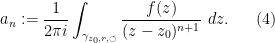
Now that we have Cauchy’s theorem, we use it to quickly give a large number of striking consequences. We begin with a special case of the Cauchy integral formula.

Theorem 17 (Cauchy integral formula, special case) Let ${U}$ be an open subset of ${{\bf C}}$ , let ${f: U \rightarrow {\bf C}}$ be holomorphic, and let ${z_0}$ be a point in ${U}$ . Let ${r>0}$ be such that the closed disk ${\overline{D(z_0,r)} := \{ z \in {\bf C}: |z-z_0| \leq r \}}$ is contained in ${U}$ . Let ${\gamma}$ be a closed curve in ${U \backslash \{z_0\}}$ that is homotopic (as a closed curve, and up to reparameterisation) in ${U \backslash \{z_0\}}$ to ${\gamma_{z_0,r,\circlearrowleft}}$ in ${U}$ . Then

$\displaystyle f(z_0) = \frac{1}{2\pi i} \int_\gamma \frac{f(z)}{z-z_0}\ dz.$

Here we are already taking advantage of the ability to integrate holomorphic functions (such as ${\frac{f(z)}{z-z_0}}$ , which is holomorphic on ${U \backslash \{z_0\}}$ ) on curves ${\gamma}$ that are not necessarily rectifiable.

Note the remarkable feature here that the value of ${f}$ at some point other than that on ${\gamma}$ is completely determined by the value of ${f}$ on the curve ${\gamma}$ , which is a strong manifestation of the “rigid” or “global” nature of holomorphic functions. Such a formula is certainly not available in the real case (Cauchy’s theorem is technically true on the real line, but there is no analogue of the circular contours ${\gamma_{z_0,r,\circlearrowleft}}$ available in that setting).

Proof: Observe that for any ${0 < \varepsilon < r}$ , the circles ${\gamma_{z_0,r,\circlearrowleft}}$ and ${\gamma_{z_0,\varepsilon,\circlearrowleft}}$ are homotopic (as closed curves) in ${\overline{D(z_0,r)}}$ , and hence in ${U}$ . Since the function ${z \mapsto \frac{f(z)}{z-z_0}}$ is holomorphic on ${U \backslash \{z_0\}}$ , we conclude from Cauchy’s theorem that

$\displaystyle \int_\gamma \frac{f(z)}{z-z_0}\ dz = \int_{\gamma_{z_0,\varepsilon,\circlearrowleft}} \frac{f(z)}{z-z_0}\ dz$

As ${f}$ is complex differentiable at ${z_0}$ , there exists a finite ${M}$ such that

$\displaystyle |\frac{f(z)-f(z_0)}{z-z_0}| \leq M$

for all ${z}$ in ${\gamma_{z_0,\varepsilon,\circlearrowleft}}$ , and all sufficiently small ${\varepsilon}$ . The length of this circle is of course ${2\pi \varepsilon}$ . Applying Exercise 17(v) of Notes 2 we have

$\displaystyle | \int_{\gamma_{z_0,\varepsilon,\circlearrowleft}} \frac{f(z)-f(z_0)}{z-z_0}\ dz| \leq 2 \pi \varepsilon M.$

On the other hand, from explicit computation (cf. Example 7) we have

$\displaystyle \int_{\gamma_{z_0,\varepsilon,\circlearrowleft}} \frac{1}{z-z_0}\ dz = 2\pi i;$

putting all this together, we see that

$\displaystyle |\frac{1}{2\pi i} \int_\gamma \frac{f(z)}{z-z_0}\ dz - f(z_0)| \leq \varepsilon M.$

Sending ${\varepsilon}$ to zero, we obtain the claim. $\Box$
Note the same argument would give

$\displaystyle m f(z_0) = \frac{1}{2\pi i} \int_\gamma \frac{f(z)}{z-z_0}\ dz$

if ${\gamma}$ were homotopic to the curve ${t \mapsto z_0 + r e^{i m t}}$ : ${0 \leq t \leq 2\pi}$ rather than ${\gamma_{z_0,r,\circlearrowleft}}$ , for some integer ${m}$ . In particular, if ${\gamma}$ were homotopic to a point in ${U \backslash \{z_0\}}$ , then the right-hand side would vanish.

Remark 18 For various explicit examples of closed contours ${\gamma}$ , it is also possible to prove the Cauchy integral formula by applying Cauchy’s theorem to various “keyhole contours”. We will not pursue this approach here, but see for instance Chapter 2 of Stein-Shakarchi.

Exercise 19 (Mean value property and Poisson kernel) Let ${U}$ be an open subset of ${{\bf C}}$ , and let ${\overline{D(z_0,r)}}$ be a closed disk contained in ${U}$ .

(i) If ${f: U \rightarrow {\bf C}}$ is holomorphic, show that
$\displaystyle f(z_0) = \frac{1}{2\pi} \int_0^{2\pi} f(z_0 + re^{i\theta})\ d\theta.$

Use this to give an alternate proof of Exercise 26 from Notes 1.

(ii) If ${u: U \rightarrow {\bf R}}$ is harmonic, show that
$\displaystyle u(z_0) = \frac{1}{2\pi} \int_0^{2\pi} u(z_0 + re^{i\theta})\ d\theta.$

Use this to give an alternate proof of Theorem 25 from Notes 1.

(iii) If ${u: U \rightarrow {\bf R}}$ is harmonic, show that
$\displaystyle u(z) = \frac{1}{2\pi} \int_0^{2\pi} P( \frac{z - z_0}{re^{i\theta}} ) u(z_0 + re^{i\theta})\ d\theta$

for any ${z \in D(z_0,r)}$ , where the Poisson kernel ${P: D(0,1) \rightarrow {\bf R}}$ is defined by the formula

$\displaystyle P(z) := \mathrm{Re} \frac{1 + z}{1-z}.$

(Hint: it simplifies the calculations somewhat if one reduces to the case ${z_0=0}$ , ${r=1}$ , and ${z = s}$ for some ${0 < s < 1}$ . Then compute the integral ${\frac{1}{2\pi i} \int_{\gamma_{0,1,\circlearrowleft}} f(w) \frac{1}{2} (\frac{1+s/w}{1-s/w} + \frac{1+sw}{1-sw})\ \frac{dw}{w}}$ in two different ways, where ${f=u+iv}$ is holomorphic with real part ${u}$ .)

The first important consequence of the Cauchy integral formula is the analyticity of holomorphic functions:

Corollary 20 (Holomorphic functions are analytic) Let ${U}$ be an open subset of ${{\bf C}}$ , let ${f: U \rightarrow {\bf C}}$ be holomorphic, and let ${z_0}$ be a point in ${U}$ . Let ${r>0}$ be such that the closed disk ${\overline{D(z_0,r)} := \{ z \in {\bf C}: |z-z_0| \leq r \}}$ is contained in ${U}$ . For each natural number ${n}$ , let ${a_n}$ denote the complex number

$\displaystyle a_n := \frac{1}{2\pi i} \int_{\gamma_{z_0,r,\circlearrowleft}} \frac{f(z)}{(z-z_0)^{n+1}}\ dz. \ \ \ \ \ (4)$

Then the power series ${\sum_{n=0}^\infty a_n (z-z_0)^n}$ has radius of convergence at least ${r}$ , and converges to ${f(z)}$ inside the disk.

Proof: By continuity, there exists a finite ${M}$ such that ${|f(z)| \leq M}$ for all ${z}$ on the circle ${\gamma_{z_0,r,\circlearrowleft}}$ , which of course has length ${2\pi r}$ . From Exercise 17(v) of Notes 2 we conclude that

$\displaystyle |a_n| \leq \frac{1}{2\pi} 2\pi r \frac{M}{r^{n+1}}.$

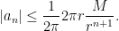
From this and Proposition 7 of Notes 1, we see that the radius of convergence of ${a_n}$ is indeed at least ${r}$ .
Next, for any ${w \in D(z_0,r)}$ , the circle ${\gamma_{z_0,r,\circlearrowleft}}$ is homotopic (as a closed curve) in ${\overline{D(z_0,r)} \backslash \{w\}}$ (and hence in ${U \backslash \{w\})}$ to ${\gamma_{w,\varepsilon,\circlearrowleft}}$ to ${\varepsilon}$ small enough that ${D(w,\varepsilon)}$ lies in ${D(z_0,r)}$ . Applying the Cauchy integral formula, we conclude that

$\displaystyle f(w) = \frac{1}{2\pi i} \int_{\gamma_{z_0,r,\circlearrowleft}} \frac{f(z)}{z-w}\ dz.$

On the other hand, from the geometric series formula (Exercise 12 of Notes 1) one has

$\displaystyle \frac{1}{z-w} = \sum_{n=0}^\infty \frac{1}{(z-z_0)^{n+1}} (w-z_0)^n$

for all ${w \in D(z_0,r)}$ , and thus

$\displaystyle f(w) = \frac{1}{2\pi i} \int_{\gamma_{z_0,r,\circlearrowleft}} (\sum_{n=0}^\infty \frac{f(z)}{(z-z_0)^{n+1}} (w-z_0)^n)\ dz.$

If we could interchange the sum and integral, we would conclude from (4) that

$\displaystyle f(w) = \sum_{n=0}^\infty a_n (w-z_0)^n$

which would give the claim. To justify the interchange, we will use the Weierstrass ${M}$ -test (the dominated convergence theorem would also work here). We have the pointwise bound

$\displaystyle |\frac{f(z)}{(z-z_0)^{n+1}} (w-z_0)^n| \leq \frac{M}{r^{n+1}} |w-z_0|^n;$

by the geometric series formula and the hypothesis 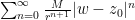${w \in D(z_0,r)}$ , the sum ${\sum_{n=0}^\infty \frac{M}{r^{n+1}} |w-z_0|^n}$ is finite, and so the ${M}$ -test applies and we are done. $\Box$

Remark 21 A function ${f: U \rightarrow {\bf C}}$ on an open set ${U \subset {\bf C}}$ is said to be complex analytic on ${U}$ if, for every ${z_0 \in U}$ , there is a power series ${\sum_{n=0}^\infty a_n(z-z_0)^n}$ with a positive radius of convergence that converges to ${f}$ on some neighbourhood of ${z_0}$ . Combining the above corollary with Theorem 15 of Notes 1, we see that ${f}$ is holomorphic on ${U}$ if and only if ${f}$ is complex analytic on ${U}$ ; thus the terms “complex differentiable”, “holomorphic”, and “complex analytic” may be used interchangeably. This can be contrasted with real variable case: there is a completely parallel notion of a real analytic function ${f: (a,b) \rightarrow {\bf R}}$ (i.e., a function such that, for every point ${x_0}$ in the domain, can be expanded as a convergent power series around that point in some neighbourhood of that point), and real analytic functions are automatically smooth and differentiable, but the converse is quite false.

Recalling (see Remark 21 of Notes 1) that power series are infinitely differentiable (in both the real and complex senses) inside their disk of convergence, and working locally in various small disks in ${U}$ , we conclude

Corollary 22 Let ${U}$ be an open subset of ${{\bf C}}$ , and let ${f: U \rightarrow {\bf C}}$ be a holomorphic function. Then ${f': U \rightarrow {\bf C}}$ is also holomorphic, and ${f}$ is smooth (i.e. infinitely differentiable in the real sense).

In view of this corollary, we may now drop hypotheses of continuous first or second differentiability from several of the theorems in Notes 1, such as Exercise 26 from that set of notes.

Combining Corollary 22 with Proposition 28 of Notes 1 (with ${{\bf C}}$ replaced by various rectangles in ${U}$ ), we obtain a form of elliptic regularity:

Corollary 23 (Elliptic regularity) Let ${U}$ be an open subset of ${{\bf C}}$ , and let ${u: U \rightarrow {\bf R}}$ be a harmonic function. Then ${u}$ is smooth.

In fact one can even omit the hypothesis of continuous twice differentiability in the definition of harmonicity if one works with the notion of weak harmonicity, but this is a topic for a PDE or distribution theory course and will not be pursued further here.

Another immediate consequence of Corollary 20 is a version of the factor theorem:

Corollary 24 (Factor theorem for analytic functions) Let ${U}$ be an open subset of ${{\bf C}}$ , and let ${z_0}$ be a point in ${{\bf C}}$ . Let ${f: U \rightarrow {\bf C}}$ be a complex analytic function that vanishes at ${z_0}$ . Then there exists a unique complex analytic function ${g: U \rightarrow {\bf C}}$ such that ${f(z) = g(z) (z-z_0)}$ for all ${z \in U}$ .

Proof: For ${z \neq z_0}$ , we can simply define ${g(z) := f(z)/(z-z_0)}$ , and this is clearly the unique choice here. For ${z}$ equal to or near ${z_0}$ , we can expand ${f}$ as a Taylor series ${f(z) = \sum_{n=1}^\infty a_n (z-z_0)^n}$ (noting that the constant term vanishes since ${f(z_0)=0}$ ) and then set ${g(z) := \sum_{n=0}^\infty a_{n+1} (z-z_0)^n}$ . One can check that these two definitions of ${g}$ agree on their common domain; on gluing the two definitions together, one obtains a function ${g}$ is complex differentiable (and hence analytic) on all of ${U}$ with the desired factorisation. Uniqueness at ${z_0}$ then follows from uniqueness at ${z \neq z_0}$ and continuity. $\Box$

Yet another consequence is the important property of analytic continuation:

Corollary 25 (Analytic continuation) Let ${U}$ be a connected non-empty open subset of ${{\bf C}}$ , and let ${f: U \rightarrow {\bf C}}$ , ${g: U \rightarrow {\bf C}}$ be complex analytic functions. If ${f}$ and ${g}$ agree on some non-empty open subset of ${U}$ , then they in fact agree on all of ${U}$ .

Proof: Let ${V}$ denote the set of all points ${z_0}$ in ${U}$ where ${f}$ and ${g}$ agree to all orders, that is to say that

$\displaystyle f^{(n)}(z_0) = g^{(n)}(z_0)$

for all ${n=0,1,\dots}$ . By hypothesis, ${V}$ is non-empty; by the continuity of the ${f^{(n)}}$ , ${V}$ is closed; and from analyticity and Taylor expansion (Exercise 17 of Notes 1) ${V}$ is open. As ${U}$ is connected, ${V}$ must therefore be all of ${U}$ , and the claim follows. (This is an example of the continuity method in action.) $\Box$
There is also a variant of the above corollary:

Corollary 26 (Non-trivial analytic functions have isolated zeroes) Let ${U}$ be a connected non-empty open subset of ${{\bf C}}$ , and let ${f: U \rightarrow {\bf C}}$ be a holomorphic function which vanishes at some point ${z_0 \in {\bf C}}$ but is not identically zero. Then there exists a disk ${D(z_0,r)}$ in ${U}$ on which ${f}$ does not vanish except at ${z_0}$ ; in other words, all the zeroes of ${f}$ are isolated points.

Proof: If all the derivatives ${f^{(n)}(z_0)}$ of ${f}$ at ${z_0}$ vanish, then by Taylor expansion ${f}$ vanishes in some open neighbourhood of ${z_0}$ , and then by Corollary 25 ${f}$ vanishes everywhere, a contradiction. Thus at least one of the ${f^{(n)}(z_0)}$ is non-zero. If ${n_0}$ is the first natural number for which ${f^{(n_0)}(z_0) \neq 0}$ , then by iterating the factor theorem (Corollary 24) we see that ${f(z) = (z-z_0)^{n_0} g(z)}$ for some analytic function ${g:U \rightarrow {\bf C}}$ which is non-vanishing at ${z_0}$ . By continuity, ${g}$ is also non-vanishing in some disk ${D(z_0,r)}$ in ${U}$ , and the claim follows. $\Box$

One particular consequence of the above corollary is that if two entire functions ${f,g}$ agree on the real line (or even on an infinite bounded subset of the complex plane), then they must agree everywhere, since otherwise ${f-g}$ would have a non-isolated zero, contradicting Corollary 26. This strengthens Corollary 25, and helps explain why real-variable identities such as ${\sin^2(x)+\cos^2(x)=1}$ automatically extend to their complex counterparts ${\sin^2(z) + \cos^2(z) = 1}$ . Another consequence is that if an entire function ${f: {\bf C} \rightarrow {\bf C}}$ is real-valued on the real axis, then one has the identity

$\displaystyle f(z) = \overline{f(\overline{z})}$

for all complex ${z}$ , because this identity already holds on the real line, and both sides are complex analytic. Thus for instance

$\displaystyle \sin(z) = \overline{\sin(\overline{z})}.$

Next, if we combine Corollary 20 with Exercise 17 of Notes 1, as well as Cauchy’s theorem, we obtain

Theorem 27 (Higher order Cauchy integral formula, special case) Let ${U}$ be an open subset of ${{\bf C}}$ , let ${f: U \rightarrow {\bf C}}$ be holomorphic, and let ${z_0}$ be a point in ${U}$ . Let ${r>0}$ be such that the closed disk ${\overline{D(z_0,r)} := \{ z \in {\bf C}: |z-z_0| \leq r \}}$ is contained in ${U}$ . Let ${\gamma}$ be a closed curve in ${U \backslash \{z_0\}}$ that is homotopic (as a closed curve, up to reparameterisation) in ${U \backslash \{z_0\}}$ to ${\gamma_{z_0,r,\circlearrowleft}}$ in ${U}$ . Then for any natural number ${n}$ , the ${n^{\mathrm{th}}}$ derivative ${f^{(n)}(z_0)}$ of ${f}$ at ${z_0}$ is given by the formula

$\displaystyle f^{(n)}(z_0) = \frac{n!}{2\pi i} \int_\gamma \frac{f(z)}{(z-z_0)^{n+1}}\ dz.$

Exercise 28 Give an alternate proof of Theorem 27 by rigorously differentiating the Cauchy integral formula with respect to the ${z_0}$ parameter.

Combining Theorem 27 with Exercise 17(v) of Notes 2, we obtain a more quantitative form of Corollary 22, which asserts not only that the higher derivatives of a holomorphic function exist, but also places a bound on them:

Corollary 29 (Cauchy inequalities) Let ${U}$ be an open subset of ${{\bf C}}$ , let ${f: U \rightarrow {\bf C}}$ be holomorphic, and let ${z_0}$ be a point in ${U}$ . Let ${r>0}$ be such that the closed disk ${\overline{D(z_0,r)} := \{ z \in {\bf C}: |z-z_0| \leq r \}}$ is contained in ${U}$ . Suppose that there is an ${M}$ such that ${|f(z)| \leq M}$ on the circle ${\{ z \in {\bf C}: |z-z_0| = r\}}$ . Then for any natural number ${n}$ , we have

$\displaystyle |f^{(n)}(z_0)| \leq \frac{n!}{r^n} M. \ \ \ \ \ (5)$

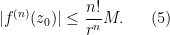
Note that the ${n=0}$ case of this corollary is compatible with the maximum principle (Exercise 26 of Notes 1).

The right-hand side of (5) has a denominator ${r^n}$ that improves when ${r}$ gets large. In particular we have the remarkable theorem of Liouville:

Theorem 30 (Liouville’s theorem) Let ${f: {\bf C} \rightarrow {\bf C}}$ be an entire function that is bounded. Then ${f}$ is constant.

Proof: By hypothesis, there is a finite ${M}$ such that ${|f(z)| \leq M}$ for all ${M}$ . Applying the Cauchy inequalities with ${n=1}$ and any disk ${D(z_0,r)}$ , we conclude that

$\displaystyle |f'(z_0)| \leq \frac{M}{r}$

for any ${z_0 \in {\bf C}}$ and ${r>0}$ . Sending ${r}$ to infinity, we conclude that ${f'}$ vanishes identically. The claim then follows from the fundamental theorem of calculus. $\Box$
This theorem displays a strong “rigidity” property for entire functions; if such a function is even vaguely close to being constant (by being bounded), then it almost magically “snaps into place” and actually is forced to be a constant! This is in stark contrast to the real case, in which there are functions such as ${\sin(x)}$ that are differentiable (and even smooth and analytic) on the real line and bounded, but definitely not constant. Note that the complex analogue ${\sin(z)}$ of the sine function is not a counterexample to Liouville’s theorem, since ${\sin(z)}$ becomes quite unbounded away from the real axis (Exercise 16 of Notes 0). This also fits well with the intuition of harmonic functions (and hence also holomorphic functions) being “balanced” in that any convexity in one direction has to be balanced by concavity in the orthogonal direction, and vice versa (as discussed before Theorem 25 of Notes 1): any attempt to create an entire function that is bounded and oscillating in one direction will naturally force that function to become unbounded in the orthogonal direction.

Exercise 31 Let ${f: {\bf C} \rightarrow {\bf C}}$ be an entire function which is of polynomial growth in the sense that there exists a finite quantity ${M>0}$ and some exponent ${A \geq 0}$ such that ${|f(z)| \leq M (1+|z|)^A}$ for all ${z \in {\bf C}}$ . Show that ${f}$ is, in fact, a polynomial.

Now we can prove the fundamental theorem of algebra discussed back in Notes 0.

Theorem 32 (Fundamental theorem of algebra) Let

$\displaystyle P(z) = a_n z^n + \dots + a_0$

be a polynomial of degree ${n \geq 0}$ for some ${a_0,\dots,a_n \in {\bf C}}$ with ${a_n}$ non-zero. Then there exist complex numbers ${z_1,\dots,z_n}$ such that

$\displaystyle P(z) = a_n (z-z_1) \dots (z-z_n).$

Proof: This is trivial for ${n=0,1}$ , so suppose inductively that ${n \geq 2}$ and the claim has already been proven for ${n-1}$ . Suppose first that the equation ${P(z)=0}$ has no roots in the complex plane, then the function ${1/P(z)}$ is entire. Also, this function goes to zero as ${|z| \rightarrow \infty}$ , and so is bounded on the exterior of any sufficiently large disk; as it is also continuous, it is bounded on any disk and is thus bounded everywhere. By Liouville’s theorem, ${1/P(z)}$ is constant, which implies that ${P(z)}$ is constant, which is absurd (for instance, the ${n^{\mathrm{th}}}$ derivative of ${P}$ is the non-zero function ${n! a_n}$ ). Hence ${P(z)}$ has at least one root ${z_n}$ . By the factor theorem (which works in any field, including the complex numbers) we can then write ${P(z) = Q(z) (z-z_n)}$ for some polynomial ${Q(z)}$ , which by the long division algorithm (or by comparing coefficients) must take the form

$\displaystyle Q(z) = a_n z^{n-1} + b_{n-2} z^{n-2} + \dots + b_0$

for some complex numbers ${b_0,\dots,b_{n-2}}$ . The claim then follows from the induction hypothesis. $\Box$
The following exercises show that ${{\bf C}}$ can be alternatively defined as an algebraic closure of the reals ${{\bf R}}$ (together with a designated square root ${i}$ of ${-1}$ ), and that extending ${{\bf R}}$ using a different irreducible polynomial than ${x^2+1}$ would still give a field isomorphic to the complex numbers, thus supporting the notion that the complex numbers are not an arbitrary extension of the reals, but rather a quite natural and canonical one.

Exercise 33 Let ${k}$ be a field containing ${{\bf R}}$ which is a finite extension of ${{\bf R}}$ , in the sense that ${k}$ is a finite-dimensional vector space over ${{\bf R}}$ . Show that ${k}$ is isomorphic (as a field) to either ${{\bf R}}$ or ${{\bf C}}$ . (Hint: if ${\alpha}$ is some element of ${k}$ not in ${{\bf R}}$ , show that ${P(\alpha)=0}$ for some irreducible polynomial ${P}$ with real coefficients but no real roots. Use this to set up an isomorphism between the field ${\tilde k}$ generated by ${{\bf R}}$ and ${\alpha}$ with ${{\bf C}}$ . If there is an element ${\beta}$ of ${k}$ not in this field ${\tilde k}$ , show that there ${Q(\beta)=0}$ for some irreducible polynomial ${Q}$ with coefficients in ${\tilde k}$ and no roots in ${\tilde k}$ , and contradict the fundamental theorem of algebra.)

Exercise 34 A field ${k}$ is said to be algebraically closed if the conclusion of Theorem 32 with ${{\bf C}}$ replaced by ${k}$ . Show that any algebraically closed field ${k}$ containing ${{\bf R}}$ , contains a subfield that is isomorphic to ${{\bf C}}$ (and which contains ${{\bf R}}$ as a subfield, isomorphic to the copy of ${{\bf R}}$ inside ${{\bf C}}$ ). Thus, up to isomorphism, ${{\bf C}}$ is the unique algebraic closure of ${{\bf R}}$ , that is to say a minimal algebraically closed field containing ${{\bf R}}$ .

Another nice consequence of the Cauchy integral formula is a converse to Cauchy’s theorem known as Morera’s theorem.

Theorem 35 (Morera’s theorem) Let ${U}$ be an open subset of ${{\bf C}}$ , and let ${f: U \rightarrow {\bf C}}$ be a continuous function. Suppose that ${f}$ is conservative in the sense that ${\int_\gamma f(z)\ dz = 0}$ for any closed polygonal path in ${U}$ . Then ${f}$ is holomorphic on ${U}$ .

Proof: By working locally with small disks in ${U}$ we may assume that ${U}$ is a disk (and in particular connected). By Exercise 32 of Notes 2, ${f}$ has an antiderivative ${F: U \rightarrow {\bf R}}$ . By definition, ${F}$ is complex differentiable at every point of ${U}$ (with derivative ${f}$ ), so by Corollary 22, ${F}$ is smooth, which implies in particular that ${F' = f}$ is holomorphic on ${U}$ as claimed. $\Box$

The power of Morera’s theorem comes from the fact that there are no differentiability requirements in the hypotheses on ${f}$ , and yet the conclusion is that ${f}$ is differentiable (and hence smooth, by Corollary 22); it can be viewed as another manifestation of “elliptic regularity”. Here is one basic application of Morera’s theorem:

Theorem 36 (Uniform limit of holomorphic functions is holomorphic) Let ${U}$ be an open subset of ${{\bf C}}$ , and let ${f_n: U \rightarrow {\bf C}}$ be a sequence of holomorphic functions that converge uniformly on compact sets to a limit ${f: U \rightarrow {\bf C}}$ . Then ${f}$ is also holomorphic. Furthermore, for any natural number ${k}$ , the derivatives ${f_n^{(k)}: U \rightarrow {\bf C}}$ also converge uniformly on compact sets to ${f^{(k)}: U \rightarrow {\bf C}}$ . (In particular, ${f_n^{(k)}}$ converges pointwise to ${f^{(k)}}$ on ${U}$ .)

Proof: Again we may work locally and assume that ${U}$ is a disk (and in partiular is convex and simply connected). The ${f_n}$ are continuous, hence their locally uniform limit ${f}$ is also continuous. From Corollary 11 (or Corollary 14), we have ${\int_\gamma f_n(z)\ dz = 0}$ on any closed polygonal path in ${U}$ , hence on taking locally uniform limits we also have ${\int_\gamma f(z)\ dz = 0}$ for such paths. The holomorphicity of ${f}$ then follows from Morera’s theorem. The uniform convergence of ${f_n^{(k)}}$ to ${f^{(k)}}$ on compact sets ${K}$ follows from applying Theorem 27 to circular contours ${\gamma_{z_0,\varepsilon,\circlearrowleft}}$ for ${z_0 \in K}$ and ${\varepsilon>0}$ small enough that these contours lie in ${U}$ (note from compactness that one can take ${\varepsilon}$ independent of ${z_0}$ ). $\Box$

Actually, one can weaken the uniform nature of the convergence in Theorem 36 substantially; even the weak limit of holomorphic functions in the space of locally integrable functions on ${U}$ will remain harmonic. However, we will not need these weaker versions of this theorem here.

Exercise 37 (Riemann’s theorem on removable singularities) Let ${U}$ be an open subset of ${{\bf C}}$ , let ${z_0}$ be a point in ${U}$ , and let ${f: U \backslash \{z_0\} \rightarrow {\bf C}}$ be a holomorphic function on ${U \backslash \{z_0\}}$ which is bounded near ${z_0}$ , in the sense that it is bounded on some punctured disk ${D(z_0,r) \backslash \{z_0\}}$ contained in ${U}$ . Show that ${f}$ has a removable singularity at ${z_0}$ , in the sense that ${f}$ is the restriction to ${U \backslash \{z_0\}}$ of a holomorphic function ${\tilde f: U \rightarrow {\bf C}}$ on ${U}$ . (Hint: show that ${f}$ is conservative near ${z_0}$ , find an antiderivative, extend it to ${U}$ , and use Morera’s theorem to show that this extension is holomorphic. Alternatively, one can also proceed by some version of the Cauchy integral formula.)

Exercise 38 (Integrals of holomorphic functions) Let ${U}$ be an open subset of ${{\bf C}}$ , and let ${f: [0,1] \times U \rightarrow {\bf C}}$ be a continuous function such that, for each ${t \in [0,1]}$ , the function ${z \mapsto f(t,z)}$ is holomorphic on ${U}$ . Show that the function ${z \mapsto \int_0^1 f(t,z)\ dt}$ is also holomorphic on ${U}$ . (Hint: work locally and use Cauchy’s theorem, Morera’s theorem, and Fubini’s theorem.)

Exercise 39 (Schwarz reflection principle) Let ${U}$ be an open subset of ${{\bf C}}$ that is symmetric around the real axis, that is to say ${\overline{z} \in U}$ whenever ${z \in U}$ . Let ${f_+: \overline{U_+} \rightarrow {\bf C}}$ be a continuous function on the set ${\overline{U_+} := \{ z \in U: \mathrm{Im}(z) \geq 0\}}$ that is holomorphic in the open subset ${U_+ := \{ z \in U: \mathrm{Im}(z) > 0 \}}$ .

(i) Suppose that ${f_-: \overline{U_-} \rightarrow {\bf C}}$ be continuous on ${\overline{U_-} := \{ z \in U: \mathrm{Im}(z) \leq 0\}}$ that is holomorphic in the open subset ${U_- := \{ z \in U: \mathrm{Im}(z) < 0 \}}$ . Suppose further that ${f_+}$ and ${f_-}$ agree on ${U \cap {\bf R}}$ . Show that ${f_+}$ and ${f_-}$ are both restrictions of a single holomorphic function ${f: U \rightarrow {\bf C}}$ .

(ii) Suppose instead that ${f_+}$ is real-valued on ${U \cap {\bf R}}$ (i.e., ${f_+(x) \in {\bf R}}$ whenever ${x \in U \cap {\bf R}}$ . Show that ${f_+}$ is the restriction of a holomorphic function ${f: U \rightarrow {\bf C}}$ , which obeys the additional property ${f(\overline{z}) = \overline{f(z)}}$ for all ${z \in U}$ .

Informally, part (ii) of this theorem asserts that one can always reflect the domain of holomorphicity of a function across a line segment on the boundary of that domain, so long as the function is continuous up to that boundary and becomes real-valued in the limit. This is the most common form of the Schwarz reflection principle.

The following two Venn diagrams (or more precisely, Euler diagrams) summarise the relationships between different types of regularity amongst continuous functions over both the reals and the complexes. The first diagram

realreg

describes the class of continuous functions on some interval ${(a,b)}$ in the real line; such functions are automatically conservative, but not necessarily differentiable, while differentiable functions are not necessarily smooth, and smooth functions are not necessarily analytic. On the other hand, when considering the class of continuous functions on an open subset ${U}$ of ${{\bf C}}$ , the picture is different:

complexreg

Now, very few continuous functions are conservative, and only slightly more functions are complex differentiable (and for simply connected domains ${U}$ , these two classes in fact coincide). Whereas in the real case, differentiable functions were considerably less regular than analytic functions, in the complex case the two classes in fact coincide.

— 3. Winding number —

One defect of the current formulation of the Cauchy integral formula (see Theorem 17 and the ensuing discussion) is that the curve ${\gamma}$ involved has to be homotopic (as a closed curve, up to reparameterisation) to a circular arc ${\gamma_{z_0,r,\circlearrowleft}}$ , or at least to a curve of the form ${t \mapsto z_0 + re^{imt}}$ , ${t \in [0,2\pi]}$ for some integer ${m}$ . We now investigate what happens when this hypothesis is removed. A key notion is that of a winding number.

Definition 40 (Winding number) Let ${\gamma}$ be a closed curve, and let ${z_0}$ be a complex number that is not in the image of ${\gamma}$ . The winding number ${W_\gamma(z_0)}$ of ${\gamma}$ around ${z_0}$ is defined by the integral

$\displaystyle W_\gamma(z_0) := \frac{1}{2\pi i} \int_\gamma \frac{dz}{z-z_0}. \ \ \ \ \ (6)$

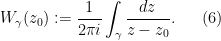
Here we again take advantage of the ability to integrate holomorphic functions on curves that are not necessarily rectifiable. Clearly the winding number is unchanged if we replace ${\gamma}$ by any equivalent curve, and if one replaces the curve ${\gamma}$ with its reversal ${-\gamma}$ , then the winding number is similarly negated. In some texts, the winding number is also referred to as the index or degree.

From the Cauchy integral formula we see that

$\displaystyle W_{\gamma}(z_0) = 1$

when ${\gamma}$ is homotopic in ${{\bf C} \backslash \{z_0\}}$ (as a closed curve, up to reparameterisation) to a circle ${\gamma_{z_0,r,\circlearrowleft}}$ , and more generally that

$\displaystyle W_{\gamma}(z_0) = m$

if ${\gamma}$ is homotopic in ${{\bf C} \backslash \{z_0\}}$ (as a closed curve, up to reparameterisation) to a curve of the form ${t \mapsto z_0 + r e^{imt}}$ , ${t \in [0,2\pi]}$ . Thus we see, intuitively at least, that ${W_\gamma(z_0)}$ measures the number of times ${\gamma}$ winds counterclockwise about ${z_0}$ , which explains the term “winding number”.
We can now state a more general form of the Cauchy integral formula:

Theorem 41 (General Cauchy integral formula) Let ${U}$ be a simply connected subset of ${{\bf C}}$ , let ${\gamma}$ be a closed curve in ${U}$ , and let ${f: U \rightarrow {\bf C}}$ be holomorphic. Then for any ${z_0}$ that lies in ${U}$ but not in the image of ${\gamma}$ , we have

$\displaystyle \frac{1}{2\pi i} \int_\gamma \frac{f(z)}{z-z_0}\ dz = W_\gamma(z_0) f(z_0).$

Proof: By Corollary 24 (or Exercise 37), we have ${f(z) - f(z_0) = (z-z_0) g(z)}$ for some holomorphic function ${g: U \rightarrow {\bf C}}$ . Hence by Theorem 14 we have

$\displaystyle \int_\gamma \frac{f(z)-f(z_0)}{z-z_0}\ dz = \int_\gamma g(z)\ dz = 0.$

The claim then follows from (6). $\Box$

Exercise 42 (Higher order general Cauchy integral formula) With ${U, \gamma, f, z_0}$ as in the above theorem, show that

$\displaystyle W_\gamma(z_0) f^{(n)}(z_0) = \frac{n!}{2\pi i} \int_\gamma \frac{f(z)}{(z-z_0)^{n+1}}\ dz$

for every natural number ${n}$ . (Hint: instead of approximating ${f(z)}$ by ${f(z_0)}$ , use a partial Taylor expansion of ${f}$ . Many of the terms that arise can be handled using the fundamental theorem of calculus. Alternatively, one can use differentiation under the integral sign and Lemma 46 below.)

To use Theorem 41, it becomes of interest to obtain more properties on the winding number. From Cauchy’s theorem we have

Lemma 43 (Homotopy invariance) Let ${z_0 \in {\bf C}}$ , and let ${\gamma_0, \gamma_1}$ be two closed curves in ${{\bf C} \backslash \{z_0\}}$ that are homotopic as closed curves up to reparameterisation in ${{\bf C} \backslash \{z_0\}}$ . Then ${W_{\gamma_0}(z_0) = W_{\gamma_1}(z_0)}$ .

The following specific corollary of this lemma will be useful for us.

Corollary 44 (Rouche’s theorem for winding number) Let ${\gamma_0: [a,b] \rightarrow {\bf C}}$ be a closed curve, and let ${z_0}$ lie outside of the image of ${\gamma_0}$ . Let ${\gamma_1: [a,b] \rightarrow {\bf C}}$ be a closed curve such that

$\displaystyle |\gamma_1(t) -\gamma_0(t)| < |\gamma_0(t) - z_0| \ \ \ \ \ (7)$

for all ${t \in [a,b]}$ . Then ${W_{\gamma_0}(z_0) = W_{\gamma}(z_0)}$ .

Proof: The map ${\gamma: [0,1] \times [a,b] \rightarrow {\bf C}}$ defined by ${\gamma(s,t) := (1-s) \gamma_0(t) + s \gamma_1(t)}$ is a homotopy from ${\gamma_0}$ to ${\gamma_1}$ ; by (7) and the triangle inequality, it avoids ${z_0}$ . The claim then follows from Lemma 43. $\Box$

Corollary 44 can be used to compute the winding number near infinity as follows. Given a curve ${\gamma: [a,b] \rightarrow {\bf C}}$ and a point ${z_0}$ , define the distance

$\displaystyle \mathrm{dist}(z_0,\gamma) := \inf_{t \in [a,b]} |z_0-\gamma(t)|$

and the diameter

$\displaystyle \mathrm{diam}(\gamma) := \sup |\gamma(t) - \gamma(t')|.$

Corollary 45 (Vanishing near infinity) Let ${\gamma}$ be a closed curve. Then ${W_\gamma(z_0) = 0}$ whenever ${z_0 \in {\bf C}}$ is such that ${\mathrm{dist}(z_0,\gamma) > \mathrm{diam}(\gamma)}$ .

Proof: Apply Corollary 44 with ${\gamma_0}$ equal to ${\gamma}$ and ${\gamma_1}$ equal to any point in the image of ${\gamma_0}$ . $\Box$

Corollary 44 also gives local constancy of the winding number:

Lemma 46 (Local constancy in ${z_0}$ ) Let ${\gamma}$ be a closed curve. Then ${W_\gamma}$ is locally constant. That is to say, if ${z_0}$ does not lie in the image of ${\gamma}$ , then there exists a disk ${D(z_0,r)}$ outside of the image of ${\gamma}$ such that ${W_\gamma(z) = W_\gamma(z_0)}$ for all ${z \in D(z_0,r)}$ .

Proof: From Corollary 44, we see that if ${r}$ is small enough and ${h \in D(0,r)}$ , then

$\displaystyle W_{\gamma-h}(z_0) = W_\gamma(z_0),$

where ${\gamma-h: t \mapsto \gamma(t)-h}$ is the translation of ${\gamma}$ by ${h}$ . But by a translation change of variables we see that

$\displaystyle W_{\gamma-h}(z_0) = W_\gamma(z_0+h)$

and the claim follows. $\Box$

Exercise 47 Give an alternate proof of Lemma 46 based on differentiation under the integral sign and using the fact that ${\frac{1}{(z-z_0)^2}}$ has an antiderivative away from ${z_0}$ .

As confirmation of the interpretation of ${W_\gamma(z_0)}$ as a winding number, we can now establish integrality:

Lemma 48 (Integrality) Let ${\gamma}$ be a closed curve, and let ${z_0}$ lie outside of the image of ${\gamma}$ . Then ${W_\gamma(z_0)}$ is an integer.

Proof: By Corollary 44 we may assume without loss of generality that ${\gamma}$ is a closed polygonal path. By partitioning a polygon into triangles (and using Lemma 46 to move ${z_0}$ slightly out of the way of any new edges formed by this partition) it suffices to verify this for triangular ${\gamma}$ . But this follows from the Cauchy integral formula (if ${z_0}$ is in the interior of the triangle) or Cauchy’s theorem (if ${z_0}$ is in the exterior). $\Box$

Exercise 49 Give another proof of Lemma 48 by restricting again to closed polygonal paths ${\gamma: [a,b] \rightarrow {\bf C}}$ , and showing that the function ${t \mapsto \exp( \int_a^t \frac{\gamma'(s)}{\gamma(s)-z_0}\ ds ) / (\gamma(t) - z_0)}$ is constant on ${[a,b]}$ by establishing that it is continuous and has vanishing derivative at all but finitely many points. (Note that ${\gamma'(s)}$ exists for all but finitely many ${s}$ , so the integral here can be well defined.)

We now come to a fundamental and well known theorem about simple closed curves, namely the Jordan curve theorem.

Theorem 50 (Jordan curve theorem) Let ${\gamma: [a,b] \rightarrow {\bf C}}$ be a non-trivial simple closed curve. Then there is an orientation ${\sigma \in \{-1,+1\}}$ such that the complex plane ${{\bf C}}$ is partitioned into the boundary region ${\gamma([a,b])}$ , the exterior region

$\displaystyle \{ z_0 \not \in \gamma([a,b]): W_\gamma(z_0) = 0 \}, \ \ \ \ \ (8)$

and the interior region

$\displaystyle \{ z_0 \not \in \gamma([a,b]): W_\gamma(z_0) = \sigma \}. \ \ \ \ \ (9)$

Furthermore:

(i) The exterior region is connected and unbounded.

(ii) The interior region is connected, non-empty and bounded.

(iii) If ${U}$ is any open set that contains ${\gamma}$ and its interior, then ${\gamma}$ is contractible to a point in ${U}$ .

(iv) The boundary of both the interior region and the exterior region is equal to the image of ${\gamma}$ .

This theorem is relatively easy to prove for “nice” curves, such as polygons, but is surprisingly delicate to prove in general. Some idea of the subtlety involved can be seen by considering pathological examples such as the lakes of Wada, which are three disjoint open connected subsets of ${{\bf C}}$ which all happen to have exactly the same boundary! This does not contradict the Jordan curve theorem, because the boundary set in this example is not given by a simple closed curve. However it does indicate that one has to carefully use the hypothesis of being a simple closed curve in order to prove Theorem 50. Another indication of the difficulty of the theorem is its global nature; the claim does not hold if one replaces the complex plane ${{\bf C}}$ by other surfaces such as the torus, the projective plane, or the Klein bottle, so the global topological structure of the complex plane must come into play at some point. For the sake of completeness, we give a proof of this theorem in an appendix to these notes.

If the quantity ${\sigma}$ in the above theorem is equal to ${+1}$ , we say that the simple closed curve ${\gamma}$ has an anticlockwise orientation; if instead ${\sigma=-1}$ we say that ${\gamma}$ has a clockwise orientation. Thus for instance, ${\gamma_{z_0,r,\circlearrowleft}}$ has an anticlockwise orientation, while its reversal ${-\gamma_{z_0,r,\circlearrowleft}}$ has the clockwise orientation.

Exercise 51 Let ${\gamma_1}$ , ${\gamma_2}$ be non-trivial simple closed curves.

(i) If ${\gamma_1,\gamma_2}$ have disjoint image, show that ${\gamma_2}$ either lies entirely in the interior of ${\gamma_1}$ , or in the exterior.

(ii) If ${\gamma_2}$ avoids the exterior of ${\gamma_1}$ , show that the interior of ${\gamma_2}$ is contained in the interior of ${\gamma_1}$ , and the exterior of ${\gamma_2}$ contains the exterior of ${\gamma_1}$ .

(iii) If ${\gamma_2}$ avoids the interior of ${\gamma_1}$ , and ${\gamma_1}$ avoids the interior of ${\gamma_2}$ , and the two curves have disjoint images, show that the interior of ${\gamma_2}$ is contained in the exterior of ${\gamma_1}$ , and the exterior of ${\gamma_2}$ contains the interior of ${\gamma_1}$ .

(This is all visually “obvious” as soon as one draws a picture, but the challenge is to provide a rigorous proof. One should of course use the Jordan curve theorem extensively to do so.)

Exercise 52 Let ${\gamma}$ be a non-trivial simple closed curve. Show that the interior of ${\gamma}$ is simply connected. (Hint: first show that any simple closed polygonal path in ${\gamma}$ is contractible to a point in the interior; then extend this to closed polygonal paths that are not necessarily simple by an induction on the number of edges in the path; then handle general closed curves.)

Remark 53 There is a refinement of the Jordan curve theorem known as the Jordan-Schoenflies theorem, that asserts that for non-trivial simple closed curve ${\gamma}$ there is a homeomorphism ${\phi: {\bf C} \rightarrow {\bf C}}$ that maps ${\gamma}$ to the unit circle ${S^1}$ , the interior of ${\gamma}$ to the unit disk ${D(0,1)}$ , and the exterior to the exterior region ${\{ z \in {\bf C}: |z| > 1 \}}$ . The proof of this improved version of the Jordan curve theorem will have to wait until we have the Riemann mapping theorem (as well as a refinement of this theorem due to Carathéodory). The Jordan-Schoenflies theorem may seem self-evident, but it is worth pointing out that the analogous result in three dimensions fails without additional regularity assumptions on the boundary surface, thanks to the counterexample of the Alexander horned sphere.

From the Jordan curve theorem we have yet another form of the Cauchy theorem and Cauchy integral formula:

Theorem 54 (Cauchy’s theorem and Cauchy integral formula for simple curves) Let ${\gamma}$ be a simple closed curve, and let ${U}$ be an open set containing ${\gamma}$ and its interior. Let ${f: U \rightarrow {\bf C}}$ be a holomorphic function.

(i) (Cauchy’s theorem) One has ${\int_\gamma f(z)\ dz = 0}$ .

(ii) (Cauchy integral formula) If ${z_0 \in U}$ lies outside of the image of ${\gamma}$ , then the expression ${\frac{1}{2\pi i} \int_\gamma \frac{f(z)}{z-z_0}\ dz}$ vanishes if ${z_0}$ lies in the exterior of ${\gamma}$ , equals ${f(z_0)}$ if ${z_0}$ lies in the interior of ${\gamma}$ and ${\gamma}$ is oriented anti-clockwise, and equals ${-f(z_0)}$ if ${z_0}$ lies in the interior of ${\gamma}$ and ${\gamma}$ is oriented clockwise.

Exercise 55 Let ${P(z) = a_n z^n + \dots + a_0}$ be a polynomial with complex coefficients ${a_0,\dots,a_n}$ and ${a_n \neq 0}$ . For any ${R>0}$ , let ${\gamma_R: [0,2\pi] \rightarrow {\bf C}}$ denote the closed contour ${\gamma_R(t) := P(R e^{it})}$ .

(i) Show that if ${R}$ is sufficiently large, then ${W_{\gamma_R}(0) = n}$ .

(ii) Show that if ${P}$ does not vanish on the closed disk ${\overline{D(0,R)}}$ , then ${W_{\gamma_R}(0)=0}$ .

(iii) Use these facts to give an alternate proof of the fundamental theorem of algebra that does not invoke Liouville’s theorem.

In the case when the closed curve ${\gamma}$ is a contour (which includes of course the case of closed polygonal paths), one can describe the interior and exterior regions, as well as the winding number, more explicitly.

Exercise 56 (Local structure of interior and exterior) Let ${\gamma = \gamma_1 + \dots + \gamma_n: [a,b] \rightarrow {\bf C}}$ be a simple closed contour formed by concatenating smooth curves ${\gamma_1,\dots,\gamma_n}$ together. Let ${z_0}$ be an interior point of one of these curves ${\gamma_i: [a_i,b_i] \rightarrow {\bf C}}$ , thus ${z_0 = \gamma_i(t_i)}$ for some ${a_i < t_i < b_i}$ . Set ${\gamma'(t_i) = re^{i\theta}}$ for some ${r>0}$ and ${\theta \in {\bf R}}$ . Recall from Exercise 25 of Notes 2 that for sufficiently small ${\varepsilon}$ , the set ${\gamma([a,b]) \cap D(z_0,\varepsilon)}$ can be expressed as a graph of the form

$\displaystyle \gamma([a,b]) \cap D(z_0,\varepsilon) = \{ z_0 + e^{i\theta} (s + i f(s)): s \in I_\varepsilon \}$

for some interval ${I_\varepsilon}$ and some continuously differentiable function ${f: I_\varepsilon \rightarrow {\bf R}}$ with ${f(0) =f'(0) = \varepsilon}$ . Show that if ${\gamma}$ is oriented anticlockwise, and ${\varepsilon}$ is sufficiently small then the interior of ${\gamma}$ contains all points in ${D(z_0,\varepsilon)}$ of the form ${z_0 + e^{i\theta} (s + i (f(s)+u))}$ for some ${s \in I_\varepsilon}$ and ${u>0}$ , and the exterior of ${\gamma}$ contains all points in ${D(z_0,\varepsilon)}$ of the form ${z_0 + e^{i\theta} (s + i (f(s)+u))}$ for some ${s \in I_\varepsilon}$ and ${u<0}$ . Similarly if ${\gamma}$ oriented clockwise, with the conditions ${u>0}$ and ${u<0}$ swapped.

Exercise 57 (Alexander numbering rule) Let ${\gamma = \gamma_1 + \dots + \gamma_n: [a,b] \rightarrow {\bf C}}$ be a closed contour formed by concatenating smooth curves ${\gamma_1,\dots,\gamma_n}$ together. Let ${\sigma = \sigma_1 + \dots + \sigma_m: [c,d] \rightarrow {\bf C}}$ be a contour formed by concatenating smooth curves ${\sigma_1,\dots,\sigma_m}$ , with initial point ${z_0}$ and terminal point ${z_1}$ . Assume that there are only finitely many points ${w_1,\dots,w_k}$ where the images of ${\gamma}$ and of ${\sigma}$ intersect. Furthermore, assume at each of the points ${w_l}$ , ${l=1,\dots,k}$ , that one has a “smooth simple transverse intersection” in the sense that the following axioms are obeyed:

(i) ${w_l}$ lies in the interior of one of the smooth curves ${\gamma_i: [a_i,b_i] \rightarrow {\bf C}}$ that make up ${\gamma}$ , thus ${w_l = \gamma_i(t_i)}$ for some ${a_i < t_i < b_i}$ .

(ii) ${w_l}$ lies in the interior of one of the smooth curves ${\sigma_j: [c_j,d_j] \rightarrow {\bf C}}$ that make up ${\sigma}$ , thus ${w_l = \sigma_j(s_j)}$ for some ${c_j < t_j < b_j}$ .

(iii) ${w_l}$ is only traversed once by ${\sigma}$ , thus there do not exist ${t \neq t'}$ in ${[c,d]}$ such that ${\sigma(t)=\sigma(t')=w_l}$ . Similarly, ${w_l}$ is only traversed once by ${\gamma}$ .

(iv) The derivatives ${\gamma'_i(t_i)}$ and ${\gamma'_j(s_j)}$ are linearly independent over ${{\bf R}}$ . In other words, we either have a crossing from the right in which ${\gamma'_j(s_j) = \lambda e^{i\theta} \gamma'_i(t_i)}$ for some ${\lambda > 0}$ and ${0 < \theta < \pi}$ , or else we have a crossing from the left in which ${\gamma'_j(s_j) = \lambda e^{i\theta} \gamma'_i(t_i)}$ for some ${\lambda > 0}$ and ${-\pi < \theta < 0}$ .

Show that ${W_\gamma(z_0) - W_\gamma(z_1)}$ is equal to the total number of crossings from the left, minus the total number of crossings from the right.

Exercise 58 Let ${U}$ be a non-empty connected open subset of ${{\bf C}}$ . Show that ${U}$ is simply connected if and only if every holomorphic function on ${U}$ is conservative.

Exercise 59 Let ${U}$ be a simply connected subset of ${{\bf C}}$ , and let ${u: U \rightarrow {\bf R}}$ be a harmonic function. Show that ${u}$ has a harmonic conjugate ${v: U \rightarrow {\bf R}}$ , which is unique up to additive constants.

Exercise 60 Let ${u: {\bf C} \rightarrow {\bf R}}$ be a harmonic function that is everywhere non-negative. Show that ${u}$ is constant. (Hint: combine ${u}$ with its harmonic conjugate and the complex exponential to create a bounded entire function.)

— 4. Appendix: proof of the Jordan curve theorem (optional) —

We now prove the Jordan curve theorem.

We first verify the claim in the easy (and visually intuitive) case that ${\gamma}$ is a non-trivial simple closed polygonal curve. Removing the polygon ${\gamma([a,b])}$ from ${{\bf C}}$ leaves an open set, which we may decompose into connected components as per Exercise 35 of Notes 2. On each of these components, the winding number ${W_\gamma}$ is constant. Since each component has a non-empty boundary that is contained in ${\gamma([a,b])}$ , this constant value of ${W_\gamma}$ must also be attained arbitrarily close to ${\gamma([a,b])}$ .

Now, a routine application of the Cauchy integral formula (see Exercise 64) shows that as ${z_0}$ crosses one of the edges of the polygon ${\gamma([a,b])}$ , the winding number ${W_\gamma(z_0)}$ is shifted by either ${+1}$ or ${-1}$ . Hence at each point ${z}$ on ${\gamma([a,b])}$ , the winding number will take two values ${\{ k, k+1\}}$ in a sufficiently small neighbourhood of ${z}$ (excluding ${\gamma([a,b])}$ ). By a continuity argument, the integer ${k}$ is independent of ${z}$ . On the other hand, from Corollary 45 the winding number must be able to attain the value of zero. Thus we have ${\{k,k+1\} = \{0,\sigma\}}$ for some ${\sigma = \pm 1}$ . Dividing a small neighbourhood of ${\gamma([a,b])}$ (excluding ${\gamma([a,b])}$ itself) into the regions where the winding numbers are ${0}$ or ${\sigma}$ , a further continuity argument shows that each of these regions lie in a single connected component. Thus there are only two connected components, one where the winding number is zero and one where the winding number is ${\sigma}$ . From (45) the latter component is bounded, hence the former is unbounded. This gives claims (i), (ii) of the Jordan curve theorem. Also, from construction we see that every point ${z}$ in ${\gamma([a,b])}$ is adherent to both the interior and exterior, giving (iv).

Now we establish claim (iii). We induct on the number ${n}$ of edges in ${\gamma}$ . The cases ${n \leq 3}$ can be handled by direct calculation, so suppose that ${n>3}$ and the claim has been proven for all smaller values of ${n}$ . We may remove any edges of zero length from the polygon. If the interior of the polygon is convex, then the claim follows from Example 2, so we may assume that the interior is non-convex. We now invoke the following geometric fact:

Exercise 61 Let ${\gamma}$ be a simple closed polygonal path with all edges of positive length. Suppose that all interior angles of ${\gamma}$ (that is, the angle that two adjacent edges make in the interior of the polygon) are less than or equal to ${\pi}$ . Show that the interior of ${\gamma}$ is convex. (Hint: first eliminate all angles that are exactly ${\pi}$ . It suffices to show that the interior is star-shaped around every interior point ${z_0}$ . To show this, first show that the set of interior points connected to ${z_0}$ by a line segment in the interior is a connected component of the interior.)

From this exercise we see that there are two adjacent edges ${e,f}$ whose interior angle exceeds ${\pi}$ . If one extends ${e}$ in the interior until it meets the polygon again, we see that this extended edge ${e^*}$ will divide the polygon into two subpolygons ${\gamma_1,\gamma_2}$ , each of which can be verified to have fewer than ${n}$ edges. Let ${\sigma_1, \sigma_2 \in \{-1,+1\}}$ be the orientations of ${\gamma_1, \gamma_2}$ . Then For any point ${z_0}$ near an interior point of the edge ${e^*}$ but not actually on ${e_*}$ , ${W_{\gamma}(z_0)}$ is equal to ${\sigma}$ , ${W_{\gamma_1}(z_0)}$ takes values in ${\{0,\sigma_1\}}$ , and ${W_{\gamma_2}(z_0)}$ takes values in ${\{0,\sigma_2\}}$ , with the latter two winding number switching as ${z_0}$ crosses ${e^*}$ . Since ${W_\gamma(z_0) = W_{\gamma_1}(z_0) + W_{\gamma_2}(z_0)}$ , we conclude that ${\sigma_1=\sigma_2=\sigma}$ , and this equation then also shows that the interiors of ${\gamma_1,\gamma_2}$ are contained in ${\gamma}$ . By induction hypothesis, ${\gamma_1}$ and ${\gamma_2}$ are contractible to a point in ${U}$ . Using Exercise 3 we conclude that ${\gamma}$ is contractible to a point in ${U}$ also.

polygon

Now we handle the significantly more difficult case when ${\gamma}$ is just a non-trivial simple closed curve. As one may expect, the strategy will be to approximate this curve by a polygonal path, but some care has to be taken when performing a limit, in order to prevent the interior region from collapsing into nothingness, or becoming disconnected, in the limit.

We begin with a variant of Corollary 44 in which the curve ${\gamma_1}$ is only required to have image close to the image of ${\gamma_0}$ , rather than be close to ${\gamma_0}$ in a pointwise (and uniform) sense. For any curve ${\gamma}$ and any ${r>0}$ , let ${N_r(\gamma) := \{ z \in {\bf C}: \mathrm{dist}(z,\gamma) < r \}}$ denote the ${r}$ -neighbourhood of ${\gamma}$ .

Proposition 62 Let ${\gamma_0}$ be a non-trivial simple closed curve, and let ${\delta>0}$ . Suppose that ${\varepsilon>0}$ is sufficiently small depending on ${\gamma_0}$ and ${\delta}$ . Let ${\gamma_1}$ be a closed curve (not necessarily simple) whose image lies in ${N_{\varepsilon}(\gamma_0)}$ . Then ${\gamma_1}$ is homotopic (as a closed curve, up to reparameterisation) to ${m\gamma_0}$ in ${N_\delta(\gamma_0)}$ , where ${m\gamma_0}$ is defined as the concatenation of ${m}$ copies of ${\gamma_0}$ if ${m}$ is positive, the trivial curve at the initial point of ${\gamma_0}$ if ${m}$ is zero, and the concatenation of ${-m}$ copies of ${-\gamma_0}$ if ${m}$ is negative. In particular, from Lemma 43 one has

$\displaystyle W_{\gamma_1}(z_0) = m W_{\gamma_0}(z_0)$

for all ${z_0 \in {\bf C} \backslash N_{\delta}(\gamma_0)}$ .

twist

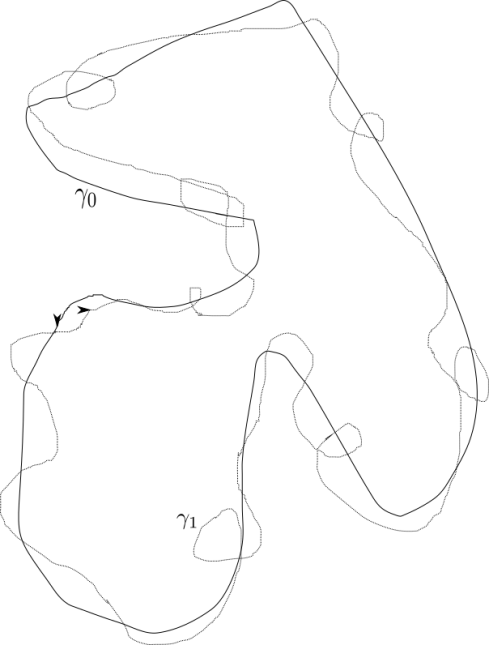
Proof: After reparameterisation, we can take ${\gamma_0: [0,1] \rightarrow {\bf C}}$ to have domain on the unit interval ${[0,1]}$ , and then by periodic extension we can view ${\gamma_0: {\bf R} \rightarrow {\bf C}}$ as a continuous ${1}$ -periodic function on ${{\bf R}}$ .

As ${[0,1]}$ is compact, ${\gamma_0}$ is uniformly continuous on ${[0,1]}$ , and hence also on ${{\bf R}}$ . In particular, there exists ${0 < \kappa < \frac{1}{10}}$ such that

$\displaystyle |\gamma_0(t_1) - \gamma_0(t_2)| \leq \frac{\delta}{2} \ \ \ \ \ (10)$

whenever ${t_1,t_2 \in {\bf R}}$ are such that ${|t_1-t_2| \leq \kappa}$ .
Fix this ${\kappa}$ . Observe that the function ${(t_1,t_2) \mapsto |\gamma_0(t_1)-\gamma_0(t_2)|}$ is continuous and nowhere vanishing on the region ${\{ (t_1,t_2) \in [0,2] \times [0,2]: \kappa \leq |t_1-t_2| \leq 1-\kappa \}}$ . Thus, if ${\varepsilon}$ is small enough depending on ${\gamma_0,\kappa}$ , we have the lower bound

$\displaystyle |\gamma_0(t_1)-\gamma_0(t_2)| \geq 3\varepsilon$

whenever ${t_1,t_2 \in [0,2]}$ are such that ${\kappa \leq |t_1-t_2| \leq 1-\kappa}$ . Using the ${1}$ -periodicity of ${\gamma_0}$ , we conclude that if ${t_1,t_2 \in {\bf R}}$ are such that

$\displaystyle |\gamma_0(t_1)-\gamma_0(t_2)| < 3\varepsilon$

the there must be an integer ${m_{t_1,t_2}}$ such that

$\displaystyle |t_2 - (t_1+m_{t_1,t_2})| < \kappa. \ \ \ \ \ (11)$

Note that this integer ${m_{t_1,t_2}}$ is uniquely determined by ${t_1}$ and ${t_2}$ .
Let ${[a,b]}$ be the domain of ${\gamma_1: [a,b] \rightarrow {\bf C}}$ . By the uniform continuity of ${\gamma_1}$ , we can find a partition ${a = s_0 < \dots < s_n = b}$ of ${[a,b]}$ such that

$\displaystyle |\gamma_1(s) - \gamma_1(s')| < \varepsilon \ \ \ \ \ (12)$

for all ${1 \leq j \leq n}$ and ${s_{j-1} \leq s, s' \leq s_j}$ . Since the image of ${\gamma_1}$ lies in ${N_{\varepsilon}(\gamma_0)}$ , we can find, for each ${0 \leq j \leq n}$ , a real number ${t_j}$ such that

$\displaystyle |\gamma_1(s_j) - \gamma_0(t_j)| < \varepsilon. \ \ \ \ \ (13)$

Since ${\gamma_1}$ is closed, we may arrange matters so that

$\displaystyle \gamma_0(t_0) = \gamma_0(t_n). \ \ \ \ \ (14)$

From the triangle inequality and (12), (13) we have

$\displaystyle |\gamma_0(t_j) - \gamma_0(t_{j-1})| < 3\varepsilon.$

Using (11), we conclude that for each ${1 \leq j \leq n}$ , there is an integer ${m_j}$ such that

$\displaystyle |t_j - (t_{j-1}+m_j)| < \kappa.$

As ${\gamma_0}$ is ${1}$ -periodic, we have the freedom to shift each of the ${t_j}$ by an arbitrary integer, and by doing this for ${t_1, \dots, t_n}$ in turn, we may assume without loss of generality that all the ${m_j}$ vanish, thus

$\displaystyle |t_j - t_{j-1}| < \kappa \ \ \ \ \ (15)$

for all ${j=1,\dots,n}$ . In particular, from (10) we have

$\displaystyle |\gamma_0(t) - \gamma_0(t')| < \frac{\delta}{2} \ \ \ \ \ (16)$

whenever ${t_{j-1} \leq t, t' \leq t_j}$ . Also, as ${\gamma_0}$ is simple, we have from (14) that

$\displaystyle t_n = t_0 + m$

for some integer ${m}$ . (Note that by enforcing (15), we no longer have the freedom to individually move ${t_0}$ or ${t_n}$ by an integer, so we cannot assume without loss of generality that ${m}$ vanishes.)
For ${j=1,\dots,n}$ , let ${\gamma_{0,j}: [j-1,j] \rightarrow {\bf C}}$ denote the curve

$\displaystyle \gamma_{0,j}(t) := \gamma_0( t_{j-1} + (t-j+1) (t_j - t_{j-1}) )$

from ${\gamma_0(t_{j-1})}$ to ${\gamma_0(t_j)}$ ; similarly let ${\gamma_{1,j}: [j-1,j] \rightarrow {\bf C}}$ denote the curve

$\displaystyle \gamma_{1,j}(t) := \gamma_1( s_{j-1} + (t-j+1) (s_j - s_{j-1}) )$

from ${\gamma_1(s_{j-1})}$ to ${\gamma_1(s_j)}$ . Observe from (16), (12), (13) that for each ${j=1,\dots,n}$ , the images of ${\gamma_{0,j}}$ and ${\gamma_{1,j}}$ both lie in ${D( \gamma_0(t_j), \frac{\delta}{2} + 3\varepsilon)}$ , which will lie in ${N_\delta(\gamma_0([a,b]))}$ if ${\varepsilon}$ is small enough. We can thus form a homotopy ${\gamma: [0,1] \times [0,n] \rightarrow N_\delta(\gamma_0([a,b]))}$ from ${\gamma_{0,1} + \dots + \gamma_{0,n}}$ to ${\gamma_{1,1} + \dots + \gamma_{1,n}}$ by defining

$\displaystyle \gamma( s, t ) = (1-s) \gamma_{0,j}(t) + s \gamma_{1,j}(t)$

for all ${1 \leq j \leq n}$ and ${j-1 \leq t \leq j}$ . Thus ${\gamma_{0,1} + \dots + \gamma_{0,n}}$ and ${\gamma_{1,1} + \dots + \gamma_{1,n}}$ are homotopic as closed curves in ${N_\delta(\gamma_0([a,b]))}$ . But by Exercise 3, ${\gamma_{0,1} + \dots + \gamma_{0,n}}$ is homotopic up to reparameterisation as closed curves to ${m \gamma_0}$ in ${N_\delta(\gamma_0([a,b]))}$ , and ${\gamma_{1,1} + \dots + \gamma_{1,n}}$ is similarly homotopic up to reparameterisation as closed curves to ${\gamma_1}$ in ${N_\delta(\gamma_0([a,b]))}$ , and the claim follows. $\Box$
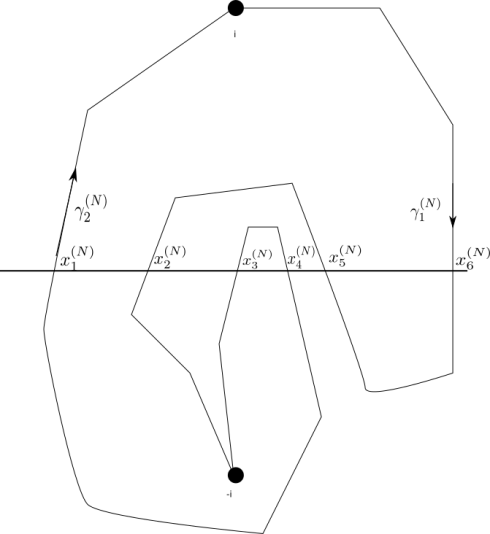
Returning to the general case of the Jordan curve theorem, we need to ensure that there is at least one point ${z_0}$ outside of ${\gamma([a,b])}$ in which ${W_f(z_0)}$ is non-zero. This is actually rather tricky; we will achieve this by a parity argument (loosely inspired by a nonstandard version of this argument from this paper of Kanovei and Reeken). Clearly, ${\gamma([a,b])}$ contains at least two points; by an appropriate rotation, translation, and dilation we may assume that ${\gamma([a,b])}$ contains the points ${+i}$ and ${-i}$ , with ${i}$ being both the initial point and the terminal point. Then we can decompose ${\gamma = \gamma_1 + \gamma_2}$ , where ${\gamma_1: [a,c] \rightarrow {\bf C}}$ is a curve from ${i}$ to ${-i}$ , and ${\gamma_2: [c,b] \rightarrow {\bf C}}$ is a curve from ${-i}$ to ${i}$ .

cut

Observe from the simplicity of ${\gamma}$ that ${|\gamma_1(t_1) - \gamma_2(t_2)| > 0}$ whenever ${t_1 \in [a,c]}$ and ${t_2 \in [c,b]}$ are such that

$\displaystyle |\mathrm{Im}(\gamma_1(t))|, |\mathrm{Im}(\gamma_2(t_2))| \leq \frac{1}{2}. \ \ \ \ \ (17)$

Thus, by compactness, there exists ${0 < \delta < \frac{1}{10}}$ such that one has the lower bound

$\displaystyle |\gamma_1(t_1) - \gamma_2(t_2)| \geq \delta \ \ \ \ \ (18)$

separating ${\gamma_1}$ from ${\gamma_2}$ whenever ${t_1 \in [a,c]}$ , ${t_2 \in [c,b]}$ are such that (17) holds.
Next, for any natural number ${N}$ , we may approximate ${\gamma: [a,b] \rightarrow {\bf C}}$ by a polygonal closed path ${\gamma^{(N)}: [a,b] \rightarrow {\bf C}}$ with

$\displaystyle |\gamma^{(N)}(t) - \gamma(t)| < \frac{1}{N} \ \ \ \ \ (19)$

for all ${t \in [a,b]}$ . Although it is not particularly necessary, we can ensure that ${\gamma^{(N)}(a) = \gamma(a) = i}$ and ${\gamma^{(N)}(c) = \gamma(c) = -i}$ . By perturbing the edges of the polygonal path ${\gamma^{(N)}}$ slightly, we may assume that none of the vertices of ${\gamma^{(N)}}$ lie on the real axis, and that none of the self-crossings of ${\gamma^{(N)}}$ (if any exist) lie on the real axis; thus, whenever ${\gamma^{(N)}}$ crosses the real axis, it does so at an interior point of an edge, with no other edge of ${\gamma^{(N)}}$ passing through that point. Note that we do not assert that the curve ${\gamma^{(N)}}$ is simple; with some more effort one could “prune” ${\gamma^{(N)}}$ by deleting short loops to make it simple, but this turns out to be unnecessary for the parity argument we give below.
Let ${x^{(N)}_1 < x^{(N)}_2 < \dots < x^{(N)}_{n^{(N)}}}$ be the points on the real axis where ${\gamma^{(N)}}$ crosses. By Exercise 64 below, the winding number ${W_{\gamma^{(N)}}(x)}$ changes by ${+1}$ or ${-1}$ as ${x}$ crosses each of the ${x^{(N)}_j}$ ; by Lemma 46, this winding number is constant otherwise, and by Corollary 45 it vanishes near infinity. Thus ${n^{(N)}}$ is even, and the winding number is odd between ${x^{(N)}_j}$ and ${x^{(N)}_{j+1}}$ for any odd ${j}$ .

Next, observe that each point ${x^{(N)}_j}$ belongs to exactly one of the polygonal paths ${\gamma^{(N)}([a,c])}$ or ${\gamma^{(N)}([c,b])}$ . Since each of these curves starts on one side of the real axis and ends up on the other, they must both cross the real axis an odd number of times. On the other hand, the crossing points ${x^{(N)}_1,\dots,x^{(N)}_n}$ can be grouped into pairs ${\{x^{(N)}_j,x^{(N)}_{j+1}\}}$ with ${j}$ odd. We conclude that there must exist an odd ${j}$ such that one of the ${x^{(N)}_j,x^{(N)}_{j+1}}$ lies in ${\gamma^{(N)}([a,c])}$ and the other lies in ${\tilde \gamma([c,b])}$ .

Fix such a ${j}$ . For sake of discussion let suppose that ${x^{(N)}_j}$ lies in ${\gamma^{(N)}([a,c])}$ and ${x^{(N)}_{j+1}}$ lies in ${\gamma^{(N)}([c,b])}$ . From (19) we have

$\displaystyle \mathrm{dist}( x^{(N)}_j, \gamma([a,c]) ) \leq \frac{1}{N}; \quad \mathrm{dist}( x^{(N)}_{j+1}, \gamma([c,b]) ) \leq \frac{1}{N}$

and from (18) we have

$\displaystyle \mathrm{dist}( x, \gamma([a,c]) ) + \mathrm{dist}( x, \gamma([c,b]) ) \geq \delta.$

for any ${x \in [x^{(N)}_j, x^{(N)}_{j+1}]}$ . By the intermediate value theorem, we can thus (for ${N}$ large enough) find ${x^{(N)}_j < x^{(N)}_* < x^{(N)}_{j+1}}$ such that

$\displaystyle \mathrm{dist}( x^{(N)}_*, \gamma([a,c]) ) = \mathrm{dist}( x^{(N)}_*, \gamma([c,b]) )$

and thus

$\displaystyle \mathrm{dist}( x^{(N)}_*, \gamma([a,c]) ), \mathrm{dist}( x^{(N)}_*, \gamma([c,b]) ) \geq \frac{\delta}{2}$

or equivalently

$\displaystyle \mathrm{dist}( x^{(N)}_*, \gamma([a,b]) ) \geq \frac{\delta}{2}.$

We arrive at the same conclusion in the opposite case when ${x^{(N)}_j}$ lies in ${\gamma^{(N)}([c,b])}$ and ${x^{(N)}_{j+1}}$ lies in ${\gamma^{(N)}([a,c])}$ .
By Corollary 45 (and (19)), the ${x^{(N)}_*}$ are bounded in ${N}$ . By the Bolzano-Weierstrass theorem, we can thus extract a subsequence of the ${x^{(N)}_*}$ that converges to some limit ${x_*}$ . By continuity we then have

$\displaystyle \mathrm{dist}( x_*, \gamma([a,b]) ) \geq \frac{\delta}{2},$

in particular ${x_*}$ does not lie in ${\gamma([a,b])}$ . By construction of ${x^{(N)}_*}$ , we know that ${W_{\gamma^{(N)}}( x^{(N)}_* )}$ is odd for all ${N}$ ; using Lemma 46 and Lemma 44 we conclude that ${W_\gamma(x_*)}$ is also odd. Thus we have found at least one point where the winding number is non-zero.
Now we can finish the proof of the Jordan curve theorem. Let ${\gamma: [a,b] \rightarrow {\bf C}}$ be a non-trivial simple closed curve. By the preceding discussion, we can find a point ${z_*}$ outside of ${\gamma([a,b])}$ where the winding number ${W_\gamma}$ is non-zero. Let ${\delta > 0}$ be a sufficiently small parameter, and let ${0 < \varepsilon = \varepsilon(\delta) < \delta}$ be sufficiently small depending on ${\delta}$ . By compactness, one can cover the region ${N_{\varepsilon/10}(\gamma([a,b]))}$ by a finite number of (solid) squares ${S}$ of sidelength ${\varepsilon/10}$ and sides parallel to the real and imaginary axes; by perturbation we may assume that no edge of one square is collinear to an edge of any other square. These squares all lie in ${N_\varepsilon(\gamma([a,b]))}$ , and in particular will not contain ${z_*}$ if ${\delta}$ is small enough; their union can easily be seen to be connected. The boundaries of these squares divide the complex plane into a finite number of polygonal regions (one of whom is unbounded). One of these regions, call it ${\Omega_\delta}$ , contains the point ${z_*}$ . This region cannot contain any interior point of a square ${S}$ , since otherwise ${\Omega_\delta}$ would be trapped inside a square of sidelength ${\varepsilon/10}$ and hence not contain ${z_*}$ . In particular, ${\Omega_\delta}$ avoids ${N_{\varepsilon/10}(\gamma([a,b]))}$ . The region ${\Omega_\delta}$ cannot be unbounded, since one could then continuously move ${z_*}$ to infinity without ever meeting ${\gamma([a,b])}$ , contradicting Lemma 46, Corollary 45, and the non-vanishing nature of ${W_\gamma(z_*)}$ . The boundary of ${\Omega_\delta}$ consists of one or more disjoint closed polygonal paths, whose edges consist of horizontal and vertical line segments. Actually, the boundary must consist of just one closed path, since otherwise the union of the squares ${S}$ would be disconnected, a contradiction. Let ${\gamma_\delta}$ denote the path that bounds ${\Omega_\delta}$ (traversed in either of the two possible directions). This path must be simple, because a crossing can only be formed by an edge of one square ${S}$ crossing an edge of another square ${S'}$ at a point that is not on the corner of either of the two squares; as ${\Omega_\delta}$ avoids both ${S}$ and ${S'}$ , it can thus only occupy one quadrant of a neighbourhood of this crossing and so cannot bound all four edges of the crossing.

square

Applying the Jordan curve theorem to the polygonal path ${\gamma_\delta}$ , we conclude that there is ${\sigma_\delta \in \{-1,+1\}}$ such that ${W_{\gamma_\delta}(z) = \sigma_\delta}$ on ${\Omega_\delta}$ , and ${W_{\gamma_\delta}(z) = 0}$ for all ${z}$ outside of ${\Omega_\delta}$ and ${\tilde \gamma([a,b])}$ . On the other hand, by Proposition 62 there is an integer ${m_\delta}$ such that ${\gamma_\delta}$ is homotopic (as closed curves, up to reparameterisation) in ${N_\delta([a,b])}$ to ${m_\delta \gamma}$ , so in particular

$\displaystyle W_{\gamma_\delta}(z) = m_\delta W_\gamma(z)$

for all ${z \not \in N_\delta(\gamma([a,b]))}$ . Applying this to ${z = z_*}$ , we conclude that ${m_\delta}$ is either ${+1}$ or ${-1}$ . If we write ${\sigma_\delta = m_\delta \sigma}$ (where ${\sigma}$ , a priori, may depend on ${\delta}$ ), then ${\sigma \in \{-1,+1\}}$ , and we have

$\displaystyle W_\gamma(z) = \sigma \ \ \ \ \ (20)$

for ${z \in \Omega_\delta \backslash N_\delta(\gamma([a,b]))}$ , and

$\displaystyle W_\gamma(z) = 0 \ \ \ \ \ (21)$

for ${z \in ({\bf C} \backslash \Omega) \backslash N_\delta(\gamma([a,b]))}$ . Thus ${W_\gamma}$ takes only two values outside of ${N_\delta(\gamma([a,b]))}$ . Sending ${\delta \rightarrow 0}$ , we conclude that ${\sigma}$ is in fact independent of ${\delta}$ , and ${W_\gamma}$ takes only the two values ${0, \sigma}$ outside of ${\gamma([a,b])}$ .
We now define the interior and exterior regions by (9), (8), then we have partitioned ${{\bf C}}$ into the interior, exterior, and ${\gamma([a,b])}$ . From Lemma 46 the interior and exterior are open, and from Lemma 45 the interior is bounded, and hence the exterior is unbounded. The point ${z_*}$ lies in the interior, so the interior is non-empty. The only remaining task to show is that the interior and exterior are connected. Suppose for instance that ${z_1, z_2}$ lie in the interior region. Then for ${\delta}$ small enough, ${z_1, z_2}$ lie outside of ${N_\delta(\gamma([a,b]))}$ . From (20), (21) we conclude that ${z_1,z_2}$ lie in ${\Omega_\delta}$ . As ${\Omega_\delta}$ is connected, we can thus join ${z_1}$ to ${z_2}$ by a path in ${\Omega_\delta}$ . As the region ${\Omega_\delta}$ avoids ${N_{\varepsilon(\delta)/10}(\gamma([a,b]))}$ , we see from Lemma 46 that the winding number ${W_\gamma}$ stays constant on this path, and so the path remains in the interior region (9). This establishes the connectedness of the interior region; the connectedness of the exterior is proven similarly. This gives (i), (ii).

Now we show (iii). Let ${\delta > 0}$ be a small parameter. As before, we can find a simple polygonal path ${\gamma_\delta}$ whose interior ${\Omega_\delta}$ lies in the interior of ${\gamma}$ , and such that ${\gamma_\delta}$ is homotopic to ${m_\delta \gamma}$ in ${N_\delta(\gamma([a,b]))}$ , and hence in ${U}$ if ${\delta}$ is small enough, for some ${m_\delta = \pm 1}$ . From the previous discussion we see that ${\gamma_\delta}$ is contractible to a point in ${U}$ , and so ${m_\delta \gamma}$ is also. The claim then follows (after reversing the contour ${m_\delta \gamma}$ if necessary).

Finally, we show (iv). We need the following variant of the Jordan curve theorem.

Exercise 63 (Jordan arc theorem) Let ${\gamma: [a,b] \rightarrow {\bf C}}$ be a simple non-closed curve. Show that the complement of ${\gamma([a,b])}$ in ${{\bf C}}$ is connected. (Hint: first establish a variant of Proposition 62 for non-closed curves, in which ${m}$ is now set to zero. Then adapt the proof of the Jordan curve theorem.)

We now show that every point ${z_0}$ in the image of ${\gamma}$ is a boundary point of the interior; the argument for the exterior is similar. If ${z_0}$ was not a boundary point of the interior, then one could remove a small neighborhood of ${z_0}$ from the image of the curve ${\gamma}$ and still disconnect the interior from the exterior. In particular (after shifting the starting and ending points of ${\gamma}$ if necessary) we could find an arc in ${\gamma}$ which disconnects the interior from the exterior; but this contradicts the Jordan arc theorem. This gives (iv), and completes the proof of the general case of the Jordan curve theorem.

Exercise 64 Let ${\gamma}$ be a non-trivial simple closed polygonal curve, and let ${z_0}$ be a point in the interior of an edge ${e}$ of ${\gamma}$ (i.e., ${z_0}$ is not one of the two vertices of ${e}$ ). Let ${z, z'}$ be two points sufficiently close to ${z_0}$ that lie on opposite sides of ${e}$ . Without using the Jordan curve theorem, show that ${|W_\gamma(z) - W_\gamma(z')| = 1}$ . (Hint: replace ${\gamma}$ by a “local” closed contour that is quite short, and a “global” closed contour which avoids the line segment connecting ${z}$ and ${z'}$ . Then use the Cauchy integral formula.)

Exercise 65 Let ${U}$ be a bounded connected non-empty open subset of ${{\bf C}}$ . Show that ${U}$ is simply connected if and only if the complement ${{\bf C} \backslash U}$ is connected. (Hint: suppose that there is a point ${z_*}$ in ${{\bf C} \backslash U}$ that is separated from infinity by ${U}$ . Show that there is some compact subset ${K}$ of ${U}$ that also separates ${z_*}$ from infinity. Then cover ${K}$ by small squares as in the proof of the Jordan curve theorem to locate a simple closed polygonal path in ${U}$ that separates ${z_*}$ from infinity.)

115 comments

Comments feed for this article

29 October, 2020 at 6:03 am

theorem 15

In proof of theorem 15, the last sentence says “if \gamma” were homotopic to a point in U\{z_0} the right hand side would vanish”. By being homotopic to a point – does it mean that one of the end points is that point? Secondly,does it vanish because it is not holomorphic in U\{z_0}?

29 October, 2020 at 7:37 am

Ben Johnsrude

Here ‘homotopic’ refers to homotopies of closed curves, so the endpoints are allowed to shift as well – that point is allowed to be any point in $U\setminus\{z_0\}$ , whether it is on the initial curve or not. The statement about vanishing is just saying that, when you integrate a continuous function around a small curve, the integral is small, so as the curve shrinks to a point the value of the integral shrinks to 0. By the assumption of holomorphicity, the value of the integral doesn’t change as the curve shrinks, so we conclude that it was 0 all along. – Ben

29 October, 2020 at 7:02 am

corollary 23

In Proof of corollary 23, analytic continuation, we have “By hypothesis, {V} is non-empty; by the continuity of the {f^{(n)}}, {V} is closed;”. Why is V closed,if {f^{(n)}} is continuous?

29 October, 2020 at 7:41 am

Ben Johnsrude

$V$ is the intersection of the sets $V_n$ , where $V_n$ is the collection of points $z$ such that $f^{(n)}(z)=g^{(n)}(z)$ ; equivalently, $V_n$ is the zero set of $f^{(n)}-g^{(n)}$ . Since the latter function is continuous, each $V_n$ is the continuous preimage of a closed set (namely, $\{0\}$ ), hence is closed. Since the intersection of closed sets is closed, $V$ is closed as well. – Ben

29 October, 2020 at 8:02 am

Anonymous

May be an alternative to Ben’s comment:

Suppose $w_m\in V$ and $w_m\to w$ . By the continuity of $f^{(n)}$ and $g^{(n)}$ , (and the definition of $V$ ), one has $f^{(n)}(w)=\lim f^{(n)}(w_m)=\lim g^{(n)}(w_m)=g^{(n)}(w)$ for all $n$ . So $w\in V$ .

On the other hand, since $\mathbb{C}$ is first countable, $w\in \overline{V}$ if and only there exists a sequence $(w_m)$ that converges to $w$ . The above argument shows that the closure $\overline{V}$ is contained in $V$ .

10 November, 2020 at 6:39 pm

Anonymous

In Exercise 53(i), one can look at the leading term $a_nz^n$ and use the Rouche’s theorem. How does one deal with 53(ii)?

11 November, 2020 at 7:58 am

Ben Johnsrude

If one pulls back the defining integral for $W_{\gamma}(0)$ by the map P, we obtain a path integral of a holomorphic function, possibly with singularities in the bounded domain. What sort of singularities appear in this case?

11 November, 2020 at 10:45 am

Anonymous

In the EX:15 on removable singularity how I can go using the given hint: show that {f} is conservative near {z_0}, find an antiderivative, extend it to {U}, and use Morera’s theorem to show that this extension is holomorphic.

1. Whether f is coneservative near z_0 means that f is conservative in D(z_0, r) \ z_0 ?

2. If the above is correct then how can I prove that integral of f over a simple closed polygonal curve winds around z_0 is 0 ?

3. And how to extended the anti derivative on hole U ?

To use morera’s theorem at first we have to show that f is continuous on U and then over any triangule in U the integral of f is 0
So, can you explain something more how to use the hypothesis so that morera’s theorem can be used.

11 November, 2020 at 11:15 am

Ben Johnsrude

1 – Yep!

2 – The important tools here will be homotopy invariance, the possibility of homotoping a curve to have very small length, and the boundedness of $f$

3 – Boundedness of $f$ translates to vanishing oscillation of the antiderivative $F$ – try and show that two distinct sequences $z_n,w_n$ limiting to the puncture $z_0$ satisfy $\lim F(z_n)=\lim F(w_n)$

To apply Morera’s theorem, I might suggest breaking an arbitrary triangle into smaller triangles on which the Cauchy integral theorem applies, at least approximately – remember, $F$ is already holomorphic on all of $\latex U\setminus\{z_0\}$!

– Ben

12 November, 2020 at 7:49 am

Anonymous

Hello Ben,
Boundedness of f makes F lipschitz on D(z_0, r) \ z_0 ??
To prove this we can follow the proof of 2nd FT of calculus.
If we have two curve joining z_1 and z_2 (with respect to a fixed point ) then /F(z_1) – F(z_2)/ bounded by M(a bound of f on punctured disk) times /z_1- z_2/.
But if the line segment joining z_1 and z_2 contains z_0 then we can’t apply triangle ineq there. So, then we go z_1 to z_2 along the same line but going avoiding z_0 by a small semi circle of radius epsilon. Then applying triangle ineq and taking epsilon as small as possible we prove our claim.(Am I correct ??)

Now we can defn F(z_0) as limit of F(z_n) as n goes to infinity for the sequence (z_n) approaches to z_0 unambiguously.
This makes F continuous on D(z_0, r) and by applying morera’s theorem then we have F is holomorphic hence f is also holomorphic.

12 November, 2020 at 9:58 am

Ben Johnsrude

That’s pretty much it! One has to be careful to check that being Lipschitz is sufficient to conclude that we do extend continuously to $z_0$ , but this fact is true.

One also has to apply Morera’s theorem correctly to conclude that $F$ is holomorphic, since we can’t assume that all integrals over closed contours are $0$ (since we don’t yet know that $F$ is holomorphic) but a standard exercise in “pushing the problem to $0$ ” will produce the desired result.

24 November, 2020 at 8:32 pm

anonymous

In the statement of Corollary 24, I think you missed mentioning that $f$ is holomorphic on $U$

[Corrected, thanks – T.]

24 November, 2020 at 9:30 pm

folkertt

I recommend that that be a standing assumption in such a section. It does not always need to be repeated: it is a waste of space and bits. But if this is intended to be a section that can be used forever and ever as a reference and in particular in the context of automated proofs, then maybe it should stay. However, the past indicates (say the King James Bible or the US constitution) that then maybe there should also be mechanisms to update and modernize the Urtext. I personally can not sleep without Newton’s Principia by my side, in Latin (edition 1 on the iPhone).

25 November, 2020 at 8:16 am

Anonymous

This information is very important !

30 November, 2020 at 5:17 pm

Anonymous

Let $U$ be a non-empty open subset of ${\bf C}$ and $\gamma:[a,b]\to{\bf C}$ a simple closed curve whose image is contained in $U$ . If $f$ is holomorphic in the interior region of $\gamma$ and continuous up to the boundary region $\gamma([a,b])$ , does one still have $\int_\gamma f(z)\,dz=0$ ?

In general, how bad can possibly $f$ behave on the boundary region given that it is holomorphic in the interior region of a simple closed curve?

4 December, 2020 at 12:38 pm

Terence Tao

For a nice enough curve (E.g., a contour) there is no difficulty since $f$ is locally uniformly continuous and one can approximate the curve by curves in the interior region in which Cauchy’s theorem already applies. If one has a non-rectifiable curve then it is not even obvious that the integral is even going to exist. There is a middle ground of curves that are rectifiable but not contours for which the answer may depend on some subtle regularity properties of the domain enclosed (one may for instance need the domain to be something like a chord-arc domain). I am not familiar enough with these sorts of low-regularity domains to say for sure though.

30 November, 2020 at 8:16 pm

Anonymous

Typo at the end of the proof of Cauchy theorem?

…where ${\gamma_{0,[t_{i-1},t_i]}: [t_{i-1},t_i] \rightarrow U}$ is the restriction of ${\gamma: [a,b] \rightarrow U}$ to ${[t_{i-1},t_i]}$ ,

… restriction of ${\gamma_0: [a,b] \rightarrow U}$ …

[Corrected, thanks -T.]

2 December, 2020 at 7:25 am

Anonymous

With the same hypotheses in Corollary 21, is it true that $u$ is also real analytic?

[Yes; this follows for instance from the Poisson kernel representation, or from viewing harmonic functions locally as real parts of holomorphic functions. -T]

2 December, 2020 at 8:36 am

Ben Johnsrude

Yep! This follows by taking the real part of the power series expansions for $u+iv$ , with $v$ a local harmonic conjugates. – Ben

2 December, 2020 at 6:57 pm

Anonymous

Typo in the proof of Morera’s theorem?

… so by Corollary 20, ${F}$ is smooth, which implies in particular that ${f' = F}$ is holomorphic on ${U}$ as claimed.

Seems more accurate to say that

… so by Corollary 20, ${F'}$ is holomorphic , which implies in particular that ${F' = f}$ is holomorphic on ${U}$ as claimed.
[Corrected, thanks – T.]

3 December, 2020 at 5:01 pm

adityaguharoy

I think there is a small typo in the statement of Lemma 41 (Homotopy invariance).
The last line should read $W_{\gamma_0} ( z_0) = W_{ \gamma_1 } (z_0)$ .

[This seems to be what is actually written in the text – T.]

5 December, 2020 at 8:18 am

adityaguharoy

Sorry my bad. I meant Corollary 42 (Rouche’s theorem).

8 December, 2020 at 9:57 am

a hardy iota guy

I think adityaguharoy referred to Corollary 42 which is namely Rouche’s theorem.

23 December, 2020 at 5:54 pm

246B, Notes 1: Zeroes, poles, and factorisation of meromorphic functions | What's new

[…] is the real part of . The claim now follows by applying the mean value property (Exercise 17 of 246A Notes 3) to […]

2 February, 2021 at 7:03 pm

246B, Notes 3: Elliptic functions and modular forms | What's new

[…] function on the punctured disk. By the Riemann singularity removal theorem (Exercise 35 of 246A Notes 3) extends to be holomorphic on all of , and thus has a Taylor expansion for some coefficients […]

12 February, 2021 at 11:27 pm

Contour shifting | Aditya Guha Roy's weblog

[…] on complex analysis; for a broader discussion on Cauchy’s theorem and its consequences refer to this blogpost by prof. Terence […]

16 February, 2021 at 3:13 am

Rex

This post seems to be missing the tag math.CV

[Corrected, thanks – T.]

12 June, 2021 at 6:48 am

Anonymous

Correction in Exercise 3 (iv) – I think we need the hypothesis that U is connected because a closed curve cannot be homotopic to a point in another component as we demand the range of the deformation to be connected.

[The point is permitted to depend on $\gamma_0$ – T.]

27 September, 2021 at 9:02 am

246A, Notes 2: complex integration | What's new

[…] Previous set of notes: Notes 1. Next set of notes: Notes 3. […]

1 November, 2021 at 12:16 am

Matt Kowalski

It seems like there’s an error with the box containing exercise 37. The box does not stop at the end of the exercise and instead continues down to contain the remainder of the post.

Also, I’m loving these notes.

[Fixed, thanks – T.]

4 November, 2021 at 1:57 pm

Siddharth M

In Exercise 47 I think the ds term should be inside the bracket on the numerator of the expression

[Corrected, thanks – T.]

22 January, 2022 at 12:35 am

Teorema de la curva de Jordan, prueba del profesor Tao - TopRespuestas

[…] Math 246A, Notes 3: Cauchy’s theorem and its consequences […]

30 April, 2022 at 8:18 am

How different is a closed curve from a 1-cycle in Exercise 15? Are they essentially the same but defined in two different languages?

30 April, 2022 at 9:45 am

Anonymous

1-cycle is a closed curve. But closed curve doesn’t have to be a 1-cycle.

1 May, 2022 at 11:13 am

Terence Tao

A 1-cycle can be decomposed as a (formal) integer linear combination of closed curves (which need not intersect each other). For instance, the sum of two disjoint oriented circles would be a 1-cycle, but not a closed curve.

	Anonymous on 275A, Notes 3: The weak and st…
	Terence Tao on 254A, Supplement 4: Probabilis…
	Anonymous on 254A, Supplement 4: Probabilis…
	Terence Tao on Analysis II
	Anonymous on Analysis II
	El problema de Erdős… on Two announcements: AI for Math…
	Anonymous on An airport-inspired puzzle
	oliverknill on Two announcements: AI for Math…
	Anonymous on An airport-inspired puzzle
	Prashant Patil on Two announcements: AI for Math…
	Anonymous on Two announcements: AI for Math…
	Anonymous on Two announcements: AI for Math…
	Anonymous on 275A, Notes 3: The weak and st…
	Anonymous on 275A, Notes 3: The weak and st…
	Anonymous on Two announcements: AI for Math…

Math 246A, Notes 3: Cauchy’s theorem and its consequences

Recent Comments

Articles by others

Diversions

Mathematics

Selected articles

Software

The sciences

Top Posts

Archives

Categories

The Polymath Blog

115 comments

Leave a reply to Ben Johnsrude Cancel reply

For commenters

Math 246A, Notes 3: Cauchy’s theorem and its consequences

Share this:

Recent Comments

Articles by others

Diversions

Mathematics

Selected articles

Software

The sciences

Top Posts

Archives

Categories

The Polymath Blog

115 comments

Leave a reply to Ben Johnsrude Cancel reply

For commenters