
Previous set of notes: Notes 3. Next set of notes: Notes 5.
In the previous set of notes we saw that functions 


Singularities come in varying levels of “badness” in complex analysis. The least harmful type of singularity is the removable singularity – a point 


After removable singularities, the mildest form of singularity one can encounter is that of a pole – an isolated singularity 


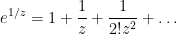
Unfortunately, there are isolated singularities that are neither removable or poles, and are known as essential singularities. A typical example is the function 


Finally, there are the non-isolated singularities. Little can be said about these singularities in general (for instance, the residue theorem does not directly apply in the presence of such singularities), but certain types of non-isolated singularities are still relatively easy to understand. One particularly common example of such non-isolated singularity arises when trying to invert a non-injective function, such as the complex exponential 


— 1. Laurent series —
Suppose we are given a holomorphic function 


 could be reconstructed from the values of on the circle by the formula
 is only known to be holomorphic outside of . Then the Cauchy integral formula no longer directly applies, because the interiors of contours such as are no longer contained in the region
  where is holomorphic. To deal with this issue, we use the following convenient decomposition.
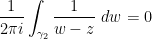
Lemma 1 (Cauchy integral formula decomposition in annular regions) Let,
be simple closed anticlockwise curves in
of
of
is contained in
on
is holomorphic on the union of
is holomorphic on the union of
as
. Furthermore, this decomposition is unique.
In addition, we have the Cauchy integral type formulae
for
for
for


Proof: We begin with uniqueness. Suppose we have two decompositions
 , where
  and
and  holomorphic, and
  both going to zero at infinity. Then the holomorphic functions
  and
and  agree on the common domain and are hence restrictions of a single entire function
  . But
. But  goes to zero at infinity and is hence bounded; applying Liouville’s theorem (Theorem 30 of Notes 3) we see that vanishes entirely. This gives
  on
on  and
and  on
on  .
.
Now for existence. Suppose that we can establish the identity (1) for 
 by
by 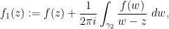 on
on  to a polygonal path) we see that is holomorphic. Similarly if we define
  on by
on by  by
by 
 obey all the required properties.
Thus it remains to establish (1). This follows from the homology form of the Cauchy integral formula (Exercise 15(v) of Notes 3), but we can also avoid explicit use of homology by the following “keyhole contour” argument. For 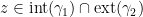


 is holomorphic.
By perturbing 


 we obtain (2) as claimed.
Exercise 2 Letbe a simple closed anticlockwise curve, and let
be simple closed anticlockwise curves in the interior
of
are also disjoint. Let
and the region
Let
, one has
(Hint: induct on
using Lemma 1.)

Exercise 3 (Painlevé’s theorem on removable singularities) Let, one can cover
such that
. Let
of
Exercise 4 (Variant of mean value theorem) Letbe a simple closed contour in
in the image of
(Hint: use the Riemann singularity removal theorem and the maximum principle.)
Now suppose that

 and
and  . From Lemma 1, we can split
  , where is holomorphic in
  , and is holomorphic in the exterior region
  , with
  going to zero as . From Corollary 20 of Notes 3, one has a Taylor expansion
 that is absolutely convergent in the disk . One cannot directly apply this Taylor expansion to . However, observe that the function
  is holomorphic in the punctured disk
  , and goes to zero as one approaches zero. By Riemann’s theorem (Exercise 37 from Notes 3), this function may be extended to
  to a holomorphic function that vanishes at the origin. Applying Corollary 20 of Notes 3 again, we conclude that there is a Taylor expansion
 that is absolutely convergent in the punctured disk . Changing variables, we conclude that
  in , and thus
  in (3), with the doubly infinite series on the right-hand side being absolutely convergent. This series is known as the Laurent series in the annulus (3). The coefficients may be explicitly computed in terms of :
Exercise 5 (Fourier inversion formula) Let, and are given by the formula
for all integers
. Also establish the bounds
and


The following modification of the above exercise may help explain the terminology “Fourier inversion formula”.
Exercise 6 (Fourier inversion formula, again) Let.
- (i) Show that if
, then we have the Fourier expansion
for all
, where the Fourier coefficients
Furthermore, show that the Fourier series in (7) is absolutely convergent, and the coefficients
- (ii) Conversely, if
are complex numbers obeying the asymptotic bounds (5), (6), show that there exists a function

The Laurent series for a given function can vary as one varies the annulus. Consider for instance the function 


 , the Taylor expansion is no longer convergent. Instead, if one writes
  and uses the geometric series formula, one instead has the Laurent expansion
Exercise 7 Find the Laurent expansions for the functionin the regions
, and
. (Hint: use partial fractions.)
We can use Laurent series to analyse an isolated singularity. Suppose that 


- (i)
such that
and
, we say that
are known as double zeroes, and so forth.
- (ii)
, and
. Poles of order
- (iii)
for infinitely many negative
It is clear that any holomorphic function 
Example 8 The functionhas a Laurent expansion
and thus has an essential singularity at
It is clear from the definition (and the holomorphicity of Taylor series) that (as discussed in the introduction), a holomorphic function 


We can now define a class of functions that only have “nice” singularities:
Definition 9 (Meromorphic functions) Letdefined on
- (i)
- (ii)
- (iii) Every
Two meromorphic functions 


Exercise 10 (Meromorphic functions form a field) Letdenote the space of meromorphic functions on a connected open set
, up to equivalence. Show that
Exercise 11 (Order is a valuation) Letof
Establish the following facts:
- (a) If
.
- (b) If
- (c) If
.
- (d) If
.
In the language of abstract algebra, the above facts are asserting that
- (i) If
for all
- (ii) If
and
. If
.
- (iii) If
. Furthermore, show if
, then the above inequality is in fact an equality.
is a valuation on the field
The behaviour of a holomorphic function near an isolated singularity depends on the type of singularity.
Theorem 12 Let
- (i) If
.
- (ii) If
as
- (iii) (Casorati-Weierstrass theorem) If
of
converging to
converges to
if
converges to
Proof: Part (i) is obvious. Part (ii) is immediate from the factorisation 


In Theorem 57 below we will establish a significant strengthening of the Casorati-Weierstrass theorem known as the Great Picard Theorem.
Exercise 13 Letbe holomorphic in
. Show that the radius of convergence of the Taylor series of
if no such non-removable singularity exists. (This fact provides a neat way to understand the rate of growth of a sequence
, locate the singularities of that function, and find out how close they get to the origin. This is a simple example of the methods of analytic combinatorics in action.)
A curious feature of the singularities in complex analysis is that the order of singularity is “quantised”: one can have a pole of order 


Exercise 14 Let,
for all
. Show that the singularity of
.) In particular, if one has
for all
As mentioned in the introduction, the theory of meromorphic functions becomes cleaner if one replaces the complex plane 
Definition 15 (Smooth manifold) Let, and let
of
(known as coordinate charts) from each
to an open subset
of
. Furthermore, the atlas is said to be smooth if for any
, the transition map
, which maps one open subset of
from one topological space
) to another
(equipped with a smooth atlas of coordinate charts
for some
) is said to be smooth if it is continuous, for any
are smooth; if
are both smooth, we say that
This definition may seem excessively complicated, but it captures the modern geometric philosophy that one should strive as much as possible to work with objects that are coordinate-independent in that they do not depend on which atlas of coordinate charts one picks within the equivalence class of the given smooth structure in order to perform computations or to define foundational concepts. One can also define smooth manifolds more abstractly, without explicit reference to atlases, by working instead with the structure sheaf of the rings 
Example 16 A simple example of a smooth; there are many equivalent atlases one could place on this circle to define the smooth structure, but one example would be the atlas consisting of the two charts
,
, defined by setting
,
,
,
,
for
, and
for
. Another smooth manifold, which turns out to be diffeomorphic to the unit circle
, is the one-point compactification
of the real numbers, with the two charts
,
,
,
to be the identity map, and
defined by setting
for
and
.
Exercise 17 Verify that the unit circle
A Riemann surface is defined similarly to a smooth manifold, except that the dimension 
Definition 18 (Riemann surface) Letare holomorphic; if
By considering dimensions
Clearly any open subset 


Now we come to the Riemann sphere 


By unpacking the definitions, we can now work out what it means for a function to be holomorphic to or from the Riemann sphere. For instance, if
- (i)
- (ii)
(which is open thanks to (i)); and
- (iii)
is holomorphic on the set
(which is open thanks to (i)), where we adopt the convention
.
Similarly, if a function 
- (i)
is holomorphic on
; and
- (ii)
is holomorphic on
, where we adopt the convention
.
We can then identify meromorphic functions with holomorphic functions on the Riemann sphere:
Exercise 19 LetFurthermore, if (ii) holds, show that
- (i)
- (ii)
to the Riemann sphere, that is not identically equal to
is uniquely determined by
Among other things, this exercise implies that the composition of two meromorphic functions is again meromorphic (outside of where the composition is undefined, of course).
Exercise 20 Letbe a holomorphic map from the Riemann sphere to itself. Show that
of one complex variable, with
for all
with
. (Hint: show that
Exercise 21 (Partial fractions) Letbe a polynomial of one complex variable, which by the fundamental theorem of algebra we may write as
for some distinct roots
, some non-zero
, and some positive integers
. Let
be another polynomial of one complex variable. Show that there exist unique polynomials
, with each
having degree less than
for
, such that one has the partial fraction decomposition
for all
. Furthermore, show that
of
of
, and has degree
otherwise.


— 2. The residue theorem —
Now we can prove a significant generalisation of the Cauchy theorem and Cauchy integral formula, known as the residue theorem.
Suppose one has a function
 . The coefficient plays a privileged role and is known as the residue of at ; we denote it by
  . Clearly this is quantity is local in the sense that it only depends on the behaviour of in a neighbourhood of ; in particular, it does not depend on the domain so long as remains inside of that domain. By convention, we also set
  if is holomorphic at (i.e., if
  ).
).
We then have
Theorem 22 (Residue theorem) Letwhere only finitely many of the terms on the right-hand side are non-zero.

Proof: Being simply connected, 


Next, we exploit the linearity of the residue theorem in 
 we see that
  for all , thus
  . Also, from the definition of winding number (see Definition 40 of Notes 3) we have
 , it thus suffices to show that
  is simply connected,
 ![{\gamma: [a,b] \rightarrow U}](https://s0.wp.com/latex.php?latex=%7B%5Cgamma%3A+%5Ba%2Cb%5D+%5Crightarrow+U%7D&bg=ffffff&fg=000000&s=0&c=20201002) is homotopic in (as closed curves) to a point. Let
is homotopic in (as closed curves) to a point. Let ![{\tilde \gamma: [0,1] \times [a,b] \rightarrow K}](https://s0.wp.com/latex.php?latex=%7B%5Ctilde+%5Cgamma%3A+%5B0%2C1%5D+%5Ctimes+%5Ba%2Cb%5D+%5Crightarrow+K%7D&bg=ffffff&fg=000000&s=0&c=20201002) denote the homotopy. We would like to mimic the proof of Cauchy’s theorem (Theorem 4 of Notes 3) to conclude (9). The difficulty is that the homotopy
denote the homotopy. We would like to mimic the proof of Cauchy’s theorem (Theorem 4 of Notes 3) to conclude (9). The difficulty is that the homotopy  may pass through points in . However, note from the vanishing of the residue
  that one has a Laurent expansion of the form
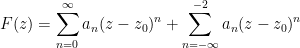
 , in some punctured disk , with both series being absolutely convergent in this punctured disk. From term by term differentiation (see Theorem 15 of Notes 1) we see that has an antiderivative in this punctured disk, namely
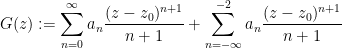
 term is absent in order to form this antiderivative). The absolute convergence of the series on the right-hand side in can be seen from the comparison test. From the fundamental theorem of calculus, we thus conclude that is conservative on . Also, for any
  that is not in , we see from Cauchy’s theorem that is conservative on for some radius
  . Putting this together using a compactness argument, we conclude that there exists a radius , such that for all in the image of the homotopy , the function is conservative in
  .
.
Now we repeat the proof of Cauchy’s theorem (Theorem 4 of Notes 3), discretising the homotopy 
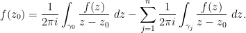
Combining the residue theorem with the Jordan curve theorem, we obtain the following special case, which is already enough for many applications:
Corollary 23 (Residue theorem for simple closed curves) LetIf


Exercise 24 (Homology version of residue theorem) Show that the residue theorem continues to hold when the closed curve.
Exercise 25 (Exterior version of residue theorem) Letconverges to a finite limit
. Show that
If


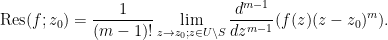
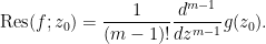
In order to use the residue theorem effectively, one of course needs some tools to compute the residue at a given point. The Fourier inversion formula (5) expresses such residues as a contour integral, but this is not so useful in practice as often the best way to compute such integrals is via the residue theorem, leaving one back where one started! But if the singularity is not an essential one, we have some useful formulae:
Exercise 26 LetUsing these facts, show that Cauchy’s theorem (Theorem 14 from Notes 3), the Cauchy integral formula (Theorem 39 from Notes 3), and the higher order Cauchy integral formula (Exercise 42 from Notes 3) can be derived from the residue theorem. (Of course, this is not an independent proof of these theorems, as they were used in the proof of the residue theorem!)
- (i) If
- (ii) If
.
- (iii) If
In particular, if
near
The residue theorem can be applied in countless ways; we give only a small sample of them below.
Exercise 27 Use the residue theorem to give an alternate proof of the fundamental theorem of algebra, by considering the integralfor a polynomial
.
Exercise 28 Letbe a Dirichlet polynomial of the form
for some sequence
of complex numbers, with only finitely many of the
for any real numbers
with
not an integer. What happens if

Exercise 29 (Spectral theorem for matrices) This exercise presumes some familiarity with linear algebra. Letdenote the ring of
complex matrices. Let
be a matrix in
, where
is the
; we let
be the distinct zeroes of this polynomial, and let
We refer to the set
as the spectrum of
- (i) Show that the resolvent
is a meromorphic function on
components are meromorphic. (Hint: use the adjugate matrix.)
- (ii) For any holomorphic
by the formula
(cf. the Cauchy integral formula). We refer to
as the holomorphic functional calculus for
is the function
, show that
Conclude in particular that if
with complex coefficients
, then the function
(as defined by the holomorphic functional calculus) matches how one would define
- (iii) Prove the Cayley-Hamilton theorem
. (Note from (ii) that it does not matter whether one interprets
algebraically, or via the holomorphic functional calculus.)
- (iv) If
has only removable singularities in
- (v) If
are holomorphic, establish the identity
- (vi) Show that there exist matrices
that are idempotent (thus
for all
), commute with each other and with
), annihilate each other (thus
for all distinct
) and are such that for each
In particular, we have the spectral decomposition
where each
is a nilpotent matrix with
. Finally, show that the range of
(viewed as a linear operator from
to itself) has dimension
. Find a way to interpret each
.


Under some additional hypotheses, it is possible to extend the analysis in the above exercise to infinite-dimensional matrices or other linear operators, but we will not do so here.
— 3. The argument principle —
We have not yet defined the complex logarithm 

 , at least away from the zeroes of . Inspired by this formal calculation, we refer to the function
  as the log-derivative of . Observe the product rule and quotient rule, when applied to complex differentiable functions
  that are non-zero at some point , gives the formulae
 , are polynomials that are factored as
 , distinct complex numbers
  , and positive integers
  , then the log-derivative of the rational function
  is given by
  is meromorphic with poles at
  , with a residue of
  at each zero of , and a residue of
  at each pole
  of .
of .
A general rule of thumb in complex analysis is that holomorphic functions behave like generalisations of polynomials, and meromorphic functions behave like generalisations of rational functions. In view of this rule of thumb and the above calculation, the following lemma should thus not be surprising:
Lemma 30 Let
- (i) If
- (ii) If
- (iii) If
- (iv) If
- (v) If
at
.
Proof: The claim (i) is obvious. For (ii), we use Taylor expansion to factor 

 is holomorphic at , the claim (ii) follows. The claim (v) is proven similarly using a factorisation , and using (12) in place of (11). The claims (iii), (iv) then follow from (i), (ii) respectively after removing the singularity.
Remark 31 Note that the lemma does not cover all possible singularity and zero scenarios. For instance,for some
). Finally, if
By combining the above lemma with the residue theorem, we obtain the argument principle:
Theorem 32 (Argument principle) Letbe a simple closed anticlockwise curve. Let
in the interior of
respectively). (
where
is the closed curve
.


Proof: The first equality of (13) follows from the residue theorem and Lemma 30. From the change of variables formula (Exercise 17(ix) of Notes 2) we have

We isolate the special case of the argument principle when there are no poles for special mention:
Corollary 33 (Special case of argument principle) Letof
around the origin.
Recalling that the winding number is a homotopy invariant (Lemma 43 of Notes 3), we conclude that the number of zeroes of a holomorphic function
Corollary 34 (Stability of number of zeroes) Let,
be simple closed anticlockwise curves that are homotopic as closed curves via some homotopy
; suppose also that
be holomorphic, and let
be a continuous function such that
and
for all
. Suppose that
for all
and
(i.e., at time
, the curve
never encounters any zeroes of
). Then the number of zeroes (counting multiplicity) of
in the interior of
Proof: By Corollary 33, it suffices to show that
![{f_0 \circ \gamma_0: [a,b] \rightarrow {\bf C} \backslash \{0\}}](https://s0.wp.com/latex.php?latex=%7Bf_0+%5Ccirc+%5Cgamma_0%3A+%5Ba%2Cb%5D+%5Crightarrow+%7B%5Cbf+C%7D+%5Cbackslash+%5C%7B0%5C%7D%7D&bg=ffffff&fg=000000&s=0&c=20201002) and
and ![{f_1 \circ \gamma_1: [a,b] \rightarrow {\bf C} \backslash \{0\}}](https://s0.wp.com/latex.php?latex=%7Bf_1+%5Ccirc+%5Cgamma_1%3A+%5Ba%2Cb%5D+%5Crightarrow+%7B%5Cbf+C%7D+%5Cbackslash+%5C%7B0%5C%7D%7D&bg=ffffff&fg=000000&s=0&c=20201002) are homotopic as closed curves in , using the homotopy
are homotopic as closed curves in , using the homotopy ![{F: [0,1] \times [a,b] \rightarrow {\bf C} \backslash \{0\}}](https://s0.wp.com/latex.php?latex=%7BF%3A+%5B0%2C1%5D+%5Ctimes+%5Ba%2Cb%5D+%5Crightarrow+%7B%5Cbf+C%7D+%5Cbackslash+%5C%7B0%5C%7D%7D&bg=ffffff&fg=000000&s=0&c=20201002) defined by
defined by 
Informally, the above corollary asserts that zeroes of holomorphic functions cannot be created or destroyed, as long as they are confined within a closed curve.
Example 35 Let. The polynomial
has a double zero at
for some
and
respectively, so as long as
, the holomorphic function
also has two zeroes in the interior of
has a double zero at the origin when
, but as soon as
Example 36 When one considers meromorphic functions instead of holomorphic ones, then the number of zeroes inside a region need not be stable any more, but the number of zeroes minus the number of poles will be stable. Consider for instance the meromorphic function, which has a removable singularity at
for some
A particularly useful special case of the stability of zeroes is Rouche’s theorem:
Theorem 37 (Rouche’s theorem) Letbe holomorphic. If one has
for all
have the same number of zeroes (counting multiplicity) in the interior of
Proof: We may assume without loss of generality that 


Rouche’s theorem has many consequences for complex analysis. One basic consequence is the open mapping theorem:
Theorem 38 (Open mapping theorem) Letis also open.
Proof: Let 


Exercise 39 Use Rouche’s theorem to obtain another proof of the fundamental theorem of algebra, by showing that a polynomialwith
inside some large circle
.)
Exercise 40 (Inverse function theorem) Let. Show that there exists a neighbourhood
of
is a complex diffeomorphism; that is to say, it is holomorphic, invertible, and the inverse is also holomorphic. Finally, show that
for all
. (Hint: one can either mimic the real-variable proof of the inverse function theorem using the contraction mapping theorem, or one can use Rouche’s theorem and the open mapping theorem to construct the inverse.)
Exercise 41 Let
- (i)
is open and
- (ii)
- (iii)
- (iv)
is nowhere vanishing.
Exercise 42 (Hurwitz’s theorem) Letbe a sequence of holomorphic functions that converge uniformly on compact sets to a limit
- (i) If none of the
have any zeroes in
- (ii) If all of the
Exercise 43 (Bloch’s theorem) The purpose of this exercise is to establish a more quantitative variant of the open mapping theorem, due to Bloch; this will be useful later in this notes for proving the Picard and Montel theorems. Letbe a holomorphic function on a disk
is non-zero
- (i) Suppose that
for all
. Show that there is an absolute constant
such that
contains the disk
. (Hint: one can normalise
,
,
. Use the higher order Cauchy integral formula to get some bound on
for
- (ii) Without the hypothesis in (i), show that there is an absolute constant
such that
. (Hint: if one has
, then we can apply (i) with
. If not, pick
with
, and start over with
. One cannot iterate this process indefinitely as it will create a singularity of
— 4. Branches of the complex logarithm —
We have refrained until now from discussing one of the most basic transcendental functions in complex analysis, the complex logarithm. In real analysis, the real logarithm 


Let’s see what happens when one tries to extend these definitions to the complex domain. We begin with the inversion of the complex exponential. From Euler’s formula we have that 


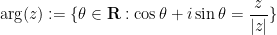 in polar form. These arguments are a coset of the group
  , and so the complex logarithm
  is a coset of the group
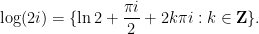
  . For instance, if
  , then
 is the empty set. As such, we will usually omit the origin from the domain when discussing the complex exponential.
Of course, one also encounters multi-valued functions in real analysis, starting when one tries to invert the squaring function 


Suppose now that we have a branch
 . If is complex differentiable at some point , then by differentiating (14) at using the chain rule, we see that

 ). If now is a closed curve in , and is differentiable on the entire image of , then the fundamental theorem of calculus then tells us that
 is equal to
  . We thus conclude that for any branch of the complex logarithm, the set on which is complex differentiable cannot contain any closed curve that winds non-trivially around the origin. Thus for instance one cannot find a branch of
  that is holomorphic on all of , or even on a neighbourhood of the unit circle (or any other curve going around the origin).
On the other hand, if 


 is connected,
  must therefore be constant; by construction we have
  , and thus
  . In other words, is a branch of the complex logarithm.
Thus, for instance, the region 


 is the standard branch of the argument, defined as the unique argument in
  in the interval
 ![{(-\pi,\pi]}](https://s0.wp.com/latex.php?latex=%7B%28-%5Cpi%2C%5Cpi%5D%7D&bg=ffffff&fg=000000&s=0&c=20201002) . This branch of the logarithm is continuous on , and hence (by the exercise below) is holomorphic on this region, and is thus an antiderivative of here; one can also extend the branch to , but it becomes discontinuous when one does so. Similarly if one replaces the negative real axis by other rays emenating from the origin (or indeed from arbitrary simple curves from zero to infinity, see Exercise 45 below.)
. This branch of the logarithm is continuous on , and hence (by the exercise below) is holomorphic on this region, and is thus an antiderivative of here; one can also extend the branch to , but it becomes discontinuous when one does so. Similarly if one replaces the negative real axis by other rays emenating from the origin (or indeed from arbitrary simple curves from zero to infinity, see Exercise 45 below.)
Exercise 44 Let
- (i) If
for all
- (ii) Show that any continuous branch
- (iii) Show that there is a continuous branch
. (Hint: for the “if” direction, use a continuity argument to show that the winding number of any closed curve in
in a compact Hausdorff space
do not lie in the same connected component, then there exists a clopen subset
Exercise 45 Letbe a continuous injective map with
and
as
.
- (i) Show that
is not all of
- (ii) Show that the complement
is simply connected. (Hint: modify the remaining arguments in Section 4 of Notes 3). In particular, by the preceding discussion, there is a branch of the complex logarithm that is holomorphic outside of
It is instructive to view the identity

 . From the fundamental theorem of calculus, one has
  that avoids the negative real axis. Of course, the contour
  does not avoid this negative axis, but it can be approximated by (non-closed) contours that do. More precisely, one has
 ![\displaystyle \int_{\gamma_{0,1,\circlearrowleft}} \frac{dz}{z} = \lim_{\varepsilon \rightarrow 0^+} \int_{\gamma_{[-\pi+\varepsilon,\pi-\varepsilon]}} \frac{dz}{z}](https://s0.wp.com/latex.php?latex=%5Cdisplaystyle++%5Cint_%7B%5Cgamma_%7B0%2C1%2C%5Ccirclearrowleft%7D%7D+%5Cfrac%7Bdz%7D%7Bz%7D+%3D+%5Clim_%7B%5Cvarepsilon+%5Crightarrow+0%5E%2B%7D+%5Cint_%7B%5Cgamma_%7B%5B-%5Cpi%2B%5Cvarepsilon%2C%5Cpi-%5Cvarepsilon%5D%7D%7D+%5Cfrac%7Bdz%7D%7Bz%7D&bg=ffffff&fg=000000&s=0&c=20201002)
![{\gamma_{[-\pi+\varepsilon,\pi-\varepsilon]}: [-\pi+\varepsilon,\pi-\varepsilon] \rightarrow {\bf C}}](https://s0.wp.com/latex.php?latex=%7B%5Cgamma_%7B%5B-%5Cpi%2B%5Cvarepsilon%2C%5Cpi-%5Cvarepsilon%5D%7D%3A+%5B-%5Cpi%2B%5Cvarepsilon%2C%5Cpi-%5Cvarepsilon%5D+%5Crightarrow+%7B%5Cbf+C%7D%7D&bg=ffffff&fg=000000&s=0&c=20201002) is the map
is the map  . As each
 ![{\gamma_{[-\pi+\varepsilon,\pi-\varepsilon]}}](https://s0.wp.com/latex.php?latex=%7B%5Cgamma_%7B%5B-%5Cpi%2B%5Cvarepsilon%2C%5Cpi-%5Cvarepsilon%5D%7D%7D&bg=ffffff&fg=000000&s=0&c=20201002) avoids the negative real axis, we thus have
avoids the negative real axis, we thus have  has a jump discontinuity of
  on the negative real axis, and specifically

 avoiding the origin can be interpreted using the standard branch of the logarithm as a version of the Alexander numbering rule (Exercise 57 of Notes 3): each crossing of across the branch cut triggers a jump up or down in the count towards the winding number, depending on whether the crossing was in the anticlockwise or clockwise direction.
One can use branches of the complex logarithm to create branches of the 


 is indeed holomorphic with
  for all . Thus for instance we have the standard branch
  of the root function, which is holomorphic away from the negative real axis. More generally, one can define a “standard branch of
  ” for any complex
  by the formula
  , for instance the standard branch of
  can be computed to be
  .
.
The presence of branch cuts can prevent one from directly applying the residue theorem to calculate integrals involving branches of multi-valued functions. But in some cases, the presence of the branch cut can actually be exploited to compute an integral. The following exercise provides an example:
Exercise 46 Compute the improper integralby applying the residue theorem to the function
for some branch
with branch cut on the positive real axis, and using a “keyhole” contour that is a perturbation of
the key point is that the branch cut makes the contribution of (the perturbations) of
and
fail to cancel each other.


The construction of holomorphic branches of
Exercise 47 Let
- (i) Show that there exists a holomorphic branch
, thus
. Furthermore, this branch is unique up to the addition of an integer multiple of
are two such branches, then
for some integer
- (ii) Show that for any natural number
, there exists a holomorphic branch
of the root function
, thus
.
Actually, one can invert other non-injective holomorphic functions than the complex exponential, provided that these functions are a covering map. We recall this topological concept:
Definition 48 (Covering map) Letbe a continuous map between two connected topological spaces
. We say that
, there exists an open neighbourhood
is the disjoint union of open subsets
of
is a homeomorphism. In this situation, we call
In complex analysis, one specialises to the situation in which 
Example 49 The exponential mapis a covering map, because for any element of
, one can pick (say) the neighbourhood
of
, and observe that the preimage
of
for
, and that the exponential map
is a diffeomorphism. A similar calculation shows that for any natural number
is not a covering map from the upper half-plane
to
around


From topology we have the following lifting property:
Lemma 50 (Lifting lemma) Letbe continuous. Let
be such that
. Then there exists a unique continuous map
such that
and
, which we call a lift of
Proof: We first verify uniqueness. If we have two continuous functions 


To verify existence of the lift, we first prove the existence of monodromy. More precisely, given any curve ![{\gamma:[a,b] \rightarrow U}](https://s0.wp.com/latex.php?latex=%7B%5Cgamma%3A%5Ba%2Cb%5D+%5Crightarrow+U%7D&bg=ffffff&fg=000000&s=0&c=20201002)

![{\tilde \gamma: [a,b] \rightarrow M}](https://s0.wp.com/latex.php?latex=%7B%5Ctilde+%5Cgamma%3A+%5Ba%2Cb%5D+%5Crightarrow+M%7D&bg=ffffff&fg=000000&s=0&c=20201002)


![{\tilde \gamma_{[a,t]}: [a,t] \rightarrow M}](https://s0.wp.com/latex.php?latex=%7B%5Ctilde+%5Cgamma_%7B%5Ba%2Ct%5D%7D%3A+%5Ba%2Ct%5D+%5Crightarrow+M%7D&bg=ffffff&fg=000000&s=0&c=20201002)
![{\tilde \gamma_{[a,t]}(a) = p}](https://s0.wp.com/latex.php?latex=%7B%5Ctilde+%5Cgamma_%7B%5Ba%2Ct%5D%7D%28a%29+%3D+p%7D&bg=ffffff&fg=000000&s=0&c=20201002)
![{f \circ \tilde \gamma_{[a,t]} = g \circ \gamma_{[a,t]}}](https://s0.wp.com/latex.php?latex=%7Bf+%5Ccirc+%5Ctilde+%5Cgamma_%7B%5Ba%2Ct%5D%7D+%3D+g+%5Ccirc+%5Cgamma_%7B%5Ba%2Ct%5D%7D%7D&bg=ffffff&fg=000000&s=0&c=20201002)
![{\gamma_{[a,t]}}](https://s0.wp.com/latex.php?latex=%7B%5Cgamma_%7B%5Ba%2Ct%5D%7D%7D&bg=ffffff&fg=000000&s=0&c=20201002)
![{[a,t]}](https://s0.wp.com/latex.php?latex=%7B%5Ba%2Ct%5D%7D&bg=ffffff&fg=000000&s=0&c=20201002)
![{[a,b]}](https://s0.wp.com/latex.php?latex=%7B%5Ba%2Cb%5D%7D&bg=ffffff&fg=000000&s=0&c=20201002)
Now let 
![{\gamma_s: [a,b] \rightarrow U}](https://s0.wp.com/latex.php?latex=%7B%5Cgamma_s%3A+%5Ba%2Cb%5D+%5Crightarrow+U%7D&bg=ffffff&fg=000000&s=0&c=20201002)

![{\tilde \gamma_s: [a,b] \rightarrow M}](https://s0.wp.com/latex.php?latex=%7B%5Ctilde+%5Cgamma_s%3A+%5Ba%2Cb%5D+%5Crightarrow+M%7D&bg=ffffff&fg=000000&s=0&c=20201002)


Since ![{\gamma_0, \gamma_1:[a,b] \rightarrow U}](https://s0.wp.com/latex.php?latex=%7B%5Cgamma_0%2C+%5Cgamma_1%3A%5Ba%2Cb%5D+%5Crightarrow+U%7D&bg=ffffff&fg=000000&s=0&c=20201002)


![{\gamma: [0,1] \rightarrow U}](https://s0.wp.com/latex.php?latex=%7B%5Cgamma%3A+%5B0%2C1%5D+%5Crightarrow+U%7D&bg=ffffff&fg=000000&s=0&c=20201002)
We can specialise this to the complex case and obtain
Corollary 51 (Holomorphic lifting lemma) Let
Proof: A Riemann surface is automatically locally path-connected, and a connected Riemann surface is automatically path connected (observe that the set of all points on the surface that can be path-connected to a reference point 
Remark 52 It is also possible to establish the above corollary using the monodromy theorem and analytic continuation.
Exercise 53 Establish Exercise 47 using Corollary 51.
Exercise 54 Letbe holomorphic and avoid taking the values
. Show that there exists a holomorphic function
. (This can be proven either through Corollary 51, or by using the quadratic formula to solve for
and then applying Exercise 47.)
In some cases it is also possible to obtain lifts in non-simply connected domains:
Exercise 55 Show that there exists a holomorphic functionsuch that
for all
. (Hint: use the Schwarz reflection principle, see Exercise 39 of Notes 3.)
As an illustration of what one can do with all this machinery, let us now prove the Picard theorems. We begin with the easier “little” Picard theorem.
Theorem 56 (Little Picard theorem) Letomits at most one point of
The example of the exponential function
Proof: Suppose for contradiction that we have an entire non-constant function 
At this point, the most natural thing to do from a Riemann surface point of view would be to cover
We turn to the details. Since 


Next, we apply Exercise 54 to write 


Now we prove the more difficult “great” Picard theorem.
Theorem 57 (Great Picard theorem) Letomits at most one point of
Note that if one only has a pole at 


Proof: This will be a variant of the proof of the little Picard theorem; it would again be more natural to use elliptic functions, but we will use some passable substitutes for such functions concocted in an ad hoc fashion out of exponential and trigonometric functions.
Assume for contradiction that 

The domain 

 is holomorphic on the right-half plane
  and avoids
  . We also observe that obeys the periodicity property
 for some holomorphic function
  , and then write
  for some holomorphic function
  that avoids all numbers of the form for natural numbers and integers . Using Bloch’s theorem as before, we see that for any disk in the right-half plane
  , we have
  for some absolute constant . We cannot set to infinity any more, but we can make as large as the real part of , giving the bound
 to
to  , and using the boundedness of
  on the compact set
  , we obtain a bound of the form
 , and all
  and
and  . Taking cosines using the formula
  , we obtain a polynomial type bound
  and .
and .
On the other hand, from (16) one has

 in the right half-plane. The set is discrete, the function
  is continuous, and the right half-plane is connected, so this function must in fact be constant. That is to say, there exists an integer such that
  in the upper half plane. Equivalently, the function
  is periodic with period . From (17) and the triangle inequality we have
  and , hence by periodicity we get this bound also for any and
  . We simplify the right-hand side somewhat as
  , and some constants
  (that can depend on , ).
We now upgrade this bound on (18) by exploiting the quantisation of pole orders (Exercise 14). As the function 
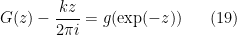
 , which is holomorphic thanks to the chain rule. From (18) we have
 . Applying Exercise 14 (with, say,
  and
and  ), we conclude that has a removable singularity and is thus in particular bounded on (say) the disk
  . From (19) we conclude that is bounded on the region ; since
  , we conclude that
  is also bounded on this region. Since
  , we conclude that
  is bounded on
  , and thus by Riemann’s theorem (Exercise 37 from Notes 3) has a removable singularity at the origin. But by taking Laurent series, this implies that has a pole of order at most at the origin, contradicting the hypothesis that the singularity of at the origin was essential.
Exercise 58 (Montel’s theorem) Letof holomorphic functions
which is uniformly convergent on compact sets (i.e., for every compact subset
that are uniformly convergent on compact sets, using the metric on the Riemann sphere induced by the identification with the geometric sphere
. (More succinctly, normal families are those families of holomorphic or meromorphic functions that are precompact in the locally uniform topology.)
- (i) (Little Montel theorem) Suppose that
there exists a constant
such that
for all
and
). Show that
- (ii) (Great Montel theorem) Let
be three distinct elements of the Riemann sphere, and suppose that
which avoid the three points
. Show that
. Then, as in the proof of the Picard theorems, express each element
and use Bloch’s theorem to get some uniform bounds on
.)
Exercise 59 (Harnack principle) Letbe a sequence of harmonic functions which is pointwise nondecreasing (thus
for all
is either infinite everywhere on
on this disk as the real part of a holomorphic function
.) This result is known as Harnack’s principle.
Exercise 60
- (i) Show that the function
is harmonic on
- (ii) Let
be a harmonic function obeying the bounds
for all
and some constants
. Show that there exists a real number
such that
for all
. (Hint: one can find a conjugate of
outside of some branch cut, say the negative real axis restricted to
. Adjust
until the conjugate becomes continuous on this branch cut.)
Exercise 61 (Local description of holomorphic maps) Let, where
is holomorphic with a simple zero at
Exercise 62 (Winding number and lifting) Letbe a closed curve avoiding
- (i)
.
- (ii) There exists a complex number
from
such that
for all
- (iii)
to the curve
that maps
to
for some

181 comments
Comments feed for this article
5 May, 2022 at 6:24 am
J
In theorem 12, is assumed to be an open subset of
  or the Riemann sphere
  ? Or for arbitrary Riemann surfaces? [In
  , since the Riemann sphere or other Riemann surfaces have not been introduced yet. However, it is not difficult to extend this theorem to those settings by using appropriate coordinate charts. -T]
5 May, 2022 at 12:37 pm
Anonymous
Typo in
… we see that has an antiderivative in this punctured disk, namely

The exponent on is
is  .
.
[Corrected, thanks – T.]
5 May, 2022 at 12:40 pm
J
[This is a natural variation of the same notation used for other infinite sums such as . -T]
. -T]