Suppose we have an  matrix
  that is expressed in block-matrix form as

where  is an
is an  matrix,
  is an
is an  matrix,
  is an
is an  matrix, and
  is a
is a  matrix for some
  . If is invertible, we can use the technique of Schur complementation to express the inverse of (if it exists) in terms of the inverse of , and the other components
  of course. Indeed, to solve the equation
where  are
are  column vectors and
  are
are  column vectors, we can expand this out as a system


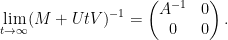
Using the invertibility of , we can write the first equation as

and substituting this into the second equation yields

and thus (assuming that  is invertible)

and then inserting this back into (1) gives

Comparing this with
we have managed to express the inverse of as


One can consider the inverse problem: given the inverse  of , does one have a nice formula for the inverse
  of the minor ? Trying to recover this directly from (2) looks somewhat messy. However, one can proceed as follows. Let
  denote the
  matrix

(with  the identity matrix), and let
  be its transpose:

Then for any scalar  (which we identify with times the identity matrix), one has

and hence by (2)

noting that the inverses here will exist for large enough. Taking limits as  , we conclude that
On the other hand, by the Woodbury matrix identity (discussed in this previous blog post), we have

and hence on taking limits and comparing with the preceding identity, one has

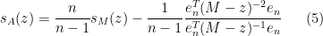
This achieves the aim of expressing the inverse of the minor in terms of the inverse of the full matrix. Taking traces and rearranging, we conclude in particular that

In the  case, this can be simplified to

where  is the
  basis column vector.
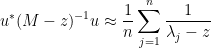
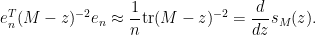
We can apply this identity to understand how the spectrum of an random matrix relates to that of its top left  minor . Subtracting any complex multiple
  of the identity from (and hence from ), we can relate the Stieltjes transform
 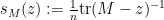 of with the Stieltjes transform
  of :
of :
At this point we begin to proceed informally. Assume for sake of argument that the random matrix is Hermitian, with distribution that is invariant under conjugation by the unitary group  ; for instance, could be drawn from the Gaussian Unitary Ensemble (GUE), or alternatively could be of the form
  for some real diagonal matrix and a unitary matrix drawn randomly from using Haar measure. To fix normalisations we will assume that the eigenvalues of are typically of size
  . Then is also Hermitian and -invariant. Furthermore, the law of
 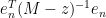 will be the same as the law of
  , where
  is now drawn uniformly from the unit sphere (independently of ). Diagonalising into eigenvalues
  and eigenvectors
  , we have

One can think of as a random (complex) Gaussian vector, divided by the magnitude of that vector (which, by the Chernoff inequality, will concentrate to  ). Thus the coefficients
  with respect to the orthonormal basis
  can be thought of as independent (complex) Gaussian vectors, divided by that magnitude. Using this and the Chernoff inequality again, we see (for distance
  away from the real axis at least) that one has the concentration of measure
and thus

(that is to say, the diagonal entries of  are roughly constant). Similarly we have
Inserting this into (5) and discarding terms of size  , we thus conclude the approximate relationship

This can be viewed as a difference equation for the Stieltjes transform of top left minors of . Iterating this equation, and formally replacing the difference equation by a differential equation in the large  limit, we see that when is large and
  for some
  , one expects the top left minor
  of to have Stieltjes transform
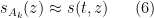
where  solves the Burgers-type equation

with initial data  .
.
Example 1 If is a constant multiple  of the identity, then
  . One checks that
  is a steady state solution to (7), which is unsurprising given that all minors of are also
  times the identity.
Example 2 If is GUE normalised so that each entry has variance  , then by the semi-circular law (see previous notes) one has
  (using an appropriate branch of the square root). One can then verify the self-similar solution
to (7), which is consistent with the fact that a top minor of also has the law of GUE, with each entry having variance  when .
One can justify the approximation (6) given a sufficiently good well-posedness theory for the equation (7). We will not do so here, but will note that (as with the classical inviscid Burgers equation) the equation can be solved exactly (formally, at least) by the method of characteristics. For any initial position  , we consider the characteristic flow
  formed by solving the ODE
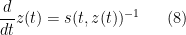
with initial data  , ignoring for this discussion the problems of existence and uniqueness. Then from the chain rule, the equation (7) implies that

and thus  . Inserting this back into (8) we see that

and thus (7) may be solved implicitly via the equation

for all and .
Remark 3 In practice, the equation (9) may stop working when 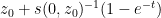 crosses the real axis, as (7) does not necessarily hold in this region. It is a cute exercise (ultimately coming from the Cauchy-Schwarz inequality) to show that this crossing always happens, for instance if has positive imaginary part then
  necessarily has negative or zero imaginary part.
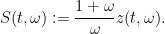
Example 4 Suppose we have  as in Example 1. Then (9) becomes
for any  , which after making the change of variables
  becomes
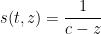
as in Example 1.
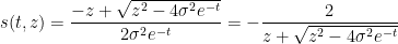
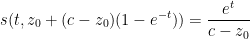
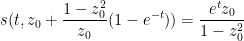
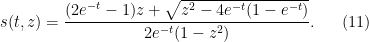
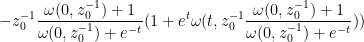
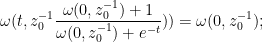
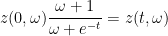
Example 5 Suppose we have
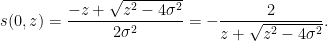
as in Example 2. Then (9) becomes

If we write

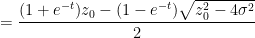
one can calculate that
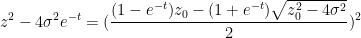
and hence
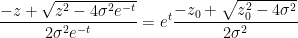
which gives

One can recover the spectral measure  from the Stieltjes transform
  as the weak limit of
  as
as  ; we write this informally as

In this informal notation, we have for instance that

which can be interpreted as the fact that the Cauchy distributions  converge weakly to the Dirac mass at as . Similarly, the spectral measure associated to (10) is the semicircular measure
  .
.
If we let  be the spectral measure associated to
  , then the curve
  from
from ![{(0,1]}](https://s0.wp.com/latex.php?latex=%7B%280%2C1%5D%7D&bg=ffffff&fg=000000&s=0&c=20201002) to the space of measures is the high-dimensional limit
to the space of measures is the high-dimensional limit  of a Gelfand-Tsetlin pattern (discussed in this previous post), if the pattern is randomly generated amongst all matrices with spectrum asymptotic to
  as . For instance, if
  , then the curve is
  , corresponding to a pattern that is entirely filled with ‘s. If instead
  is a semicircular distribution, then the pattern is

thus at height  from the top, the pattern is semicircular on the interval
 ![{[-2\sigma \sqrt{\alpha}, 2\sigma \sqrt{\alpha}]}](https://s0.wp.com/latex.php?latex=%7B%5B-2%5Csigma+%5Csqrt%7B%5Calpha%7D%2C+2%5Csigma+%5Csqrt%7B%5Calpha%7D%5D%7D&bg=ffffff&fg=000000&s=0&c=20201002) . The interlacing property of Gelfand-Tsetlin patterns translates to the claim that
. The interlacing property of Gelfand-Tsetlin patterns translates to the claim that  (resp.
  ) is non-decreasing (resp. non-increasing) in for any fixed
  . In principle one should be able to establish these monotonicity claims directly from the PDE (7) or from the implicit solution (9), but it was not clear to me how to do so.
An interesting example of such a limiting Gelfand-Tsetlin pattern occurs when  , which corresponds to being
  , where
  is an orthogonal projection to a random
  -dimensional subspace of
  . Here we have
and so (9) in this case becomes
A tedious calculation then gives the solution
For  , there are simple poles at
  , and the associated measure is

This reflects the interlacing property, which forces  of the
  eigenvalues of the
  minor to be equal to
  (resp.
  ). For
  , the poles disappear and one just has
For  , one has an inverse semicircle distribution

There is presumably a direct geometric explanation of this fact (basically describing the singular values of the product of two random orthogonal projections to half-dimensional subspaces of ), but I do not know of one off-hand.
The evolution of can also be understood using the  -transform and
  -transform from free probability. Formally, letlet
  be the inverse of , thus

for all  , and then define the -transform
The equation (9) may be rewritten as

and hence

or equivalently

See these previous notes for a discussion of free probability topics such as the -transform.
Example 6 If then the transform is  .
.
Example 7 If is given by (10), then the transform is
Example 8 If is given by (11), then the transform is

This simple relationship (12) is essentially due to Nica and Speicher (thanks to Dima Shylakhtenko for this reference). It has the remarkable consequence that when  is the reciprocal of a natural number
  , then
  is the free arithmetic mean of copies of , that is to say is the free convolution
  of copies of , pushed forward by the map
  . In terms of random matrices, this is asserting that the top
  minor of a random matrix has spectral measure approximately equal to that of an arithmetic mean
  of independent copies of , so that the process of taking top left minors is in some sense a continuous analogue of the process of taking freely independent arithmetic means. There ought to be a geometric proof of this assertion, but I do not know of one. In the limit
  (or
(or  ), the -transform becomes linear and the spectral measure becomes semicircular, which is of course consistent with the free central limit theorem.
In a similar vein, if one defines the function

and inverts it to obtain a function  with
with
for all  , then the -transform
  is defined by
Writing

for any , , we have

and so (9) becomes

which simplifies to
replacing by  we obtain

and thus
and hence
One can compute  to be the -transform of the measure
  ; from the link between -transforms and free products (see e.g. these notes of Guionnet), we conclude that
  is the free product of
  and . This is consistent with the random matrix theory interpretation, since is also the spectral measure of
  , where is the orthogonal projection to the span of the first basis elements, so in particular has spectral measure . If is unitarily invariant then (by a fundamental result of Voiculescu) it is asymptotically freely independent of , so the spectral measure of
  is asymptotically the free product of that of and of .


6 comments
Comments feed for this article
16 September, 2017 at 9:16 pm
domotorp
There’s a typo after “and then inserting this back into (1) gives”, a there should be a parenthesis around the expression multiplied by a. Also, the equation (2) is too wide and the “(2)” is not visible (for me).
[Corrected, thanks – T.]
20 September, 2017 at 7:29 am
Sergei Ofitserov
Dear Terence Tao! I again participate in discussion by theme Szemeredi’s theorem(previous post). P(1),P(2),P(3)-that directions of unfolding arithmetic progressions. More exactly,P(1) and P(2)-that unfolding of arithmetic progressions by columns up and down. Upper bound-9999, lower bound-1000(that bounds of Fourier analysis). And here P(3)-that already direction of unfolding arithmetic progressions by stitchs, wear out in infinity. P(3) for theorem1.6-that line of locking in infinity(fully possibly-closed elliptical curve). 1-1/10L-that no finished first page of my book. Thanks! Sergei.
26 September, 2017 at 10:28 am
JDM
Your inversion formulas also appear in Wikipedia. While everything is a “matrix”, my Representation Theory textbooks hardly write out the operators in this way. By drawing a column for each group element, as Cayley or Schur might have done. And lo and behold they were block diagonal !!
https://en.m.wikipedia.org/wiki/Invertible_matrix#Blockwise_inversion
https://en.m.wikipedia.org/wiki/Block_matrix
28 September, 2017 at 8:02 pm
Anonymous
A closing bracket is missing in the equation number “(2)”.
[It’s there, but cut off by the blog. -T]
2 October, 2017 at 9:52 am
burakcakmakblog
Professor, as regards the discussion below Example (8), the formula by Nica and Speicher, i.e. for
for  can be easily shown as follows: From the multiplicative free convolution we have
  . Then, by invoking the general relationship between the R- and S- transforms which is
  (see [Haagerup, Larsen, 99]) we get
  .
.
7 September, 2020 at 9:30 am
Free fractional convolution powers | What's new
[…] initial condition (see for a derivation). This equation can be solved explicitly using the emph as free probability analogues of the classical probability concepts of differential entropy and […]