This is the sixth “research” thread of the Polymath15 project to upper bound the de Bruijn-Newman constant  , continuing this post. Discussion of the project of a non-research nature can continue for now in the existing proposal thread. Progress will be summarised at this Polymath wiki page.
The last two threads have been focused primarily on the test problem of showing that  whenever
  . We have been able to prove this for most regimes of
  , or equivalently for most regimes of the natural number parameter
  . In many of these regimes, a certain explicit approximation
  to
to  was used, together with a non-zero normalising factor
  ; see the wiki for definitions. The explicit upper bound

has been proven for certain explicit expressions  (see here) depending on . In particular, if satisfies the inequality

then  is non-vanishing thanks to the triangle inequality. (In principle we have an even more accurate approximation
  available, but it is looking like we will not need it for this test problem at least.)
We have explicit upper bounds on  ,
,  ,
,  ; see this wiki page for details. They are tabulated in the range
  here. For
  , the upper bound
  for is monotone decreasing, and is in particular bounded by
  , while and are known to be bounded by
  and
and  respectively (see here).
Meanwhile, the quantity  can be lower bounded by

for certain explicit coefficients  and an explicit complex number
  . Using the triangle inequality to lower bound this by
we can obtain a lower bound of  for , which settles the test problem in this regime. One can get more efficient lower bounds by multiplying both Dirichlet series by a suitable Euler product mollifier; we have found
  for
for  to be good choices to get a variety of further lower bounds depending only on
  , see this table and this wiki page. Comparing this against our tabulated upper bounds for the error terms we can handle the range
  .
.
In the range  , we have been able to obtain a suitable lower bound
  (where
  exceeds the upper bound for
  ) by numerically evaluating at a mesh of points for each choice of , with the mesh spacing being adaptive and determined by and an upper bound for the derivative of ; the data is available here.
This leaves the final range  (roughly corresponding to
  ). Here we can numerically evaluate to high accuracy at a fine mesh (see the data here), but to fill in the mesh we need good upper bounds on
  . It seems that we can get reasonable estimates using some contour shifting from the original definition of (see here). We are close to finishing off this remaining region and thus solving the toy problem.
Beyond this, we need to figure out how to show that for  as well. General theory lets one do this for
  , leaving the region
  . The analytic theory that handles and should also handle this region; for
  presumably the argument principle will become relevant.
The full argument also needs to be streamlined and organised; right now it sprawls over many wiki pages and github code files. (A very preliminary writeup attempt has begun here). We should also see if there is much hope of extending the methods to push much beyond the bound of  that we would get from the above calculations. This would also be a good time to start discussing whether to move to the writing phase of the project, or whether there are still fruitful research directions for the project to explore.
Participants are also welcome to add any further summaries of the situation in the comments below.


102 comments
Comments feed for this article
18 March, 2018 at 8:37 pm
Terence Tao
I will be at a reduced level of activity this week as I will be involved in the opening week of activities at IPAM’s quantitative linear algebra program (including giving some tutorials in random matrix theory). I just wanted to record one observation here though. In order to use the argument principle, we need to evaluate the variation of on some rectangle, e.g. the rectangle bordering
  . We can work with
  instead (this is still holomorphic on this rectangle), as presumably this oscillates a bit less and is more numerically tractable.
Suppose we can evaluate on some mesh
  around this rectangle, with the property that for any
  between adjacent points
  on this mesh,
  . (This is basically what we are already doing with the adaptive mesh.) Then not only is it the case that
  is non-zero, but the variation
  must be between
  and
and  for any such
  , and in particular
  is just the standard branch of the argument of
  . This should allow us to compute the winding number by adding up all the variations in the argument and then dividing by
  . Alternatively one could proceed visually: if one simply joins up the
  by line segments (literally "connecting the dots") and plots them, the winding number of the true curve of
  will match the winding number of this polygonal path, which should hopefully be visibly equal to zero.
19 March, 2018 at 10:26 am
KM
I will start working on the contour calculations.
Using the stationary point Pi/8 – (1/4)*atan((9+y)/x) results in further improvement in the derivative bound, with the average mesh spacing now around 0.065 (although most of the benefit is at the lower x values).
Also, earlier there was an issue with the I integral diverging for very small x, eg. x less than 13, but now it gives correct estimates for x greater than 0.
Although the older theta value (without the 1/4 factor) seems to give more stable exact integral estimates at larger x values.
23 March, 2018 at 10:47 am
KM
I attempted to create approximate plots of H/B0 and H’/H as z is varied along the rectangle above in a counterclockwise direction with step size 0.01. (A+B-C was used to approximate H, and NQ_(A+B-C) to approximate H’). Both never wound around the origin.
H/B0 plot
H’/H plot
H’/H plot zoomed near the origin
Are these plots the right way to go, and once made rigorous with an adaptive mesh and exact estimates, can they serve as proofs (backed by scripts which can always reproduce them)?
23 March, 2018 at 12:52 pm
Terence Tao
Thanks for this! The plot looks particularly good; while there is some oscillation (which by the way I would imagine would become damped if one puts in a few Euler product mollifiers, but I doubt we need to do that) the behavior looks simple enough that we should be able to rigorously control the winding number relatively easily, given that
  stays well away from the negative real axis most of the time. As I mentioned in a previous comment, as long as the mesh
  is such that
  for all
  on the segment connecting
  to
to  , the winding number for the trajectory of
  will equal that of the polygonal path connecting the
  (this is basically Rouche's theorem), and it is visually clear from the plot that this path does not wind around the origin (and one could numerically verify this if desired by summing the argument increments). As long as the polygonal path stays some distance
  away from origin, one should be able to tolerate errors of up to
  in the approximation (another application of Rouche's theorem).
The fact that doesn't wind around the origin would give information about the zeroes of
  . The Ki-Kim-Lee paper studies this question also; the de Bruijn-Newman constant
  is in fact just the first in a sequence of constants
  where
where  concerns the Riemann hypothesis for
  ,
,  concerns the Riemann hypothesis for
  , and so forth. (See Theorem 1.2 of Ki-Kim-Lee.) It seems likely that a lot of what we do to control the zeroes of
  could also be carried over to
  , etc. (possibly with slightly better bounds on the corresponding de Bruijn-Newman constant), but I’m not sure if we have the energy to explore this direction too much (at some point it may make sense to just “declare victory” and write up what we have).
24 March, 2018 at 12:58 am
KM
Using an adaptive mesh, and the faster integral suggested by Rudolph, we get the plots below (visually, the difference from the earlier plot is that the vertices and edges of the polygon are of different color and the vertices are not equidistant). The second plot is a closeup near the origin.
Adaptive mesh plot of H/B0
Closeup near the origin
Also, the data used to generate the plot is here
24 March, 2018 at 3:37 am
Anonymous
Why the polygon seems to be almost (but not really) closed?
24 March, 2018 at 7:54 am
KM
That must be because the adaptive mesh stopped at the ‘last’ point and not at the starting point. This can be easily changed.
Also, as a contrast to the above plot, here is an animated plot (fixed mesh) for the rectangle x= 0 to 50, and y= -0.2 to 0.2, within which we know that zeroes do occur.
Animated plot for a contour containing zeroes. It winds around the origin 3 times, and is fun to watch!
24 March, 2018 at 10:10 am
Terence Tao
Thanks for this! The plot gets somewhat close to the origin, but presumably the distance is still much larger than the numerical accuracy for in this region. I’ve added links to these plots at the bottom of the test problem wiki page.
I think we will also need to conduct a similar exercise in the region in which the analytic lower bounds on
  don’t work (even with the Euler product mollifier trick). Here we would need to numerically plot
  around the rectangle and ensure that it not only fails to wind around the origin, but stays a distance at least
  away from some branch cut connecting the origin to infinity, where
  is an upper bound for the total error
  . (Based on the existing plots, the negative real axis may serve as a reasonable branch cut for this purpose, since
  seems to move away from that axis rather quickly and stay away indefinitely.) One may need to do this for each
  separately, though for the purposes of just seeing how things should look we can just plot
  for all
  at once without trying to worry about error terms and optimal mesh sizes.
25 March, 2018 at 1:12 am
KM
Data for y=0.4, N=11 to 300 was available from the earlier adaptive mesh exercise (around 6 million points), so it was reused. For y=0.45, data for around 100k points was generated. For the horizontal sides of the rectangle, a few points were easily evaluated.
These are some of the resulting plots.
(A+B)/B0 plot for y=0.4, N=11 to 300 (green vertices and red edges)
(A+B)/B0 plot for the rectangle (no edges, green vertices for y=0.4, orange vertices for y=0.45, and black vertices for the horizontal sides)
Since the y=0.45 data is too coarse, it’s vertices weren’t joined as in the first graph.
Comparing (A+B)/B0 values for y=0.4 and y=0.45, we see the latter are further away from the origin and also more tightly clustered. Minimum distance from the origin is around 0.31 (with a y=0.4 vertex), which compares favorably with the N=11 error bound of 0.163.
25 March, 2018 at 1:53 am
Anonymous
Perhaps “horizontal sides” should be “vertical sides” ?
25 March, 2018 at 8:07 am
Terence Tao
Thanks for this! The distance from the negative real axis should comfortably exceed the sum of the 0.165 error bound and the maximum fluctuation between mesh points (i.e. the derivative bound times the size of the mesh), since this was how the 0.4 mesh was designed at least.
Regarding the need to evaluate the y=0.45 data at a finer mesh, one possibility is to raise this value something larger, e.g. y=1, (thus making the rectangle a bit taller) and use analytic estimates (which improve as y increases; already when going from 0.4 to 0.45 we see that the orange dots are a bit closer to 1 than the green dots). If one is lucky one may be able to cover most of the N=11 to 300 region here. There is a catch though which is that the E_1,E_2,E_3 errors degrade exponentially as y increases (the E_3 error in particular contains an annoying factor of ), so there is a tradeoff. (Incidentally I now have slightly different values of E_1,E_2,E_3 in the pdf writeup which may be slightly better, and are designed to work for y from 0 to 1, compared to the old estimates which were valid up to
  .)
.)
Anyway, it looks like we almost have covered everything we need to prove (one could joke that we are now 4% closer to the Riemann hypothesis :). One just needs to make the meshes for the
  and
and  rectangle evaluations fine enough that (when combined with derivative bounds and error estimates) there is no possibility of unexpected winding around the origin.
25 March, 2018 at 11:20 am
KM
Thanks. Rudolph and I had started the y=0.45, N =11 to 300 adaptive mesh clockwise, which can be now be used as a backup if needed, after which we will also cover the N<11 rectangle.
Also, a minor detail is that the N=20 to 300 mesh had been run earlier (and similarly now) with c=0.065, and c=0.165 was used for N=11 to 19, which hopefully doesn't affect the results.
I tried the new e3 bound in the paper, although so far it seems to stay slightly higher than the current one. Will double check my formulas and share the update.
25 March, 2018 at 1:27 pm
Terence Tao
Yes, the bound is slightly worse mainly because it is covering a larger range, instead of
  ; also because there was a slight error in the wiki treatment (I put it in boldface in http://michaelnielsen.org/polymath1/index.php?title=Effective_bounds_on_H_t_-_second_approach#Bounding_G_.7Bt.2CN.7D.28s.29 ), which will probably also lead to some worsening if it is fixed. How bad is the degradation of the bound? There is scope to improve the bound a bit by making it a bit messier.
It’s fine to have different values of c for different meshes. Actually at the end of the day we may get better bounds away from zero than the c parameter, because we also get to use the fundamental theorem of calculus in the backwards direction too. For instance, let’s say we are trying to keep the function away from zero and we are using a mesh
  with rule
 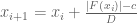 , where
  is a uniform upper bound for
  ; assume that all the mesh evaluations
  are at least
  . Then we certainly have
for . But we also have
and hence in fact we have the lower bound
which is a slightly better bound than . (In fact this suggests that one may be able to take
  or even
  slightly negative and still get a good bound, which could be a modest speedup, albeit at the cost of incurring a slight risk that the mesh is not fine enough to get a usable bound.)
25 March, 2018 at 6:09 pm
KM
These are some of the older and newer e3 bounds I am getting with y=t=0.4
N, old, new
11, 0.161, 0.181
20, 0.064, 0.080
50, 0.015, 0.021
300, 0.0007, 0.001
I will also create a table with the new e1,e2,e3 and overall error for each N.
25 March, 2018 at 10:38 pm
Terence Tao
One can replace the 1.46 in the e3 bound in Prop 5.6(vi) with , which may improve things a little bit. The 0.069 can be improved further to
 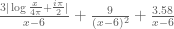 but this will probably only give a tiny gain.
26 March, 2018 at 7:18 am
Terence Tao
I’ve now updated my copy of the writeup with these sharpened bounds (and this should propagate into the main github repo soon). Furthermore, the approach now also gives a quantitative error bound for rather than
  ; the bound is the same except that the “
 ” term in the
  bound is dropped. This might give an alternate way to deal with
  just below 11 that may be more numerically efficient (which may be important as we go below 0.48).
26 March, 2018 at 11:32 am
KM
With the new improved bounds for e3 (of A+B) I get these values (t=y=0.4)
N, old, new
11, 0.161, 0.133
20, 0.064, 0.057
50, 0.015, 0.01478
300, 0.000725, 0.000720
The new bounds for e1 and e2 are sharper too.
I wasn’t completely sure about the (1-3y)+ factor in the paper, so have assumed it to be max(0,1-3y). [Yes, this is correct. -T]
A new table with e1,e2,e3_ab,e3_abc,e_toal_ab,e_total_abc is kept here
[Added to wiki, thanks – T.]
27 March, 2018 at 12:32 pm
KM
The (A+B)/B0 mesh data for N=300 to 20, y=0.45, t=0.4, c=0.065 is kept here
Also, with the improved error bounds, even N=7 works with this approach. Too avoid too many outputs and c values, I generated mesh data with c=0.26 for N=7 to 19, y=0.4,t=0.4 and N=19 to 7, y=0.45,t=0.4, which are kept here and here
For t=0.4, this leaves the rectangle upto x~620 for the integral mesh.
Assuming the derivative bound does not change much if one used the (A+B-C)/B0 mesh, it may be possible to cover N=4 to 6 as well (with different c values). As an extreme, I tried ddx_bound_ABC=10*ddx_bound_AB, and it ran with c=0.26 for N=4 and c=0.16 for N=5,6 (a uniform value of 0.26 didn’t work for N=5,6).
[Links added to test problem wiki page. -T]
18 March, 2018 at 11:36 pm
KM
Summarizing some observations on the numerical effort. For the current test problem, as already mentioned in the post, we are now into the final regime of x<=1600, where the A+B lower bound and the E1+E2+E3 upper bound start overlapping. Hence for this regime, we are using a mesh with exact numerical integration of H_t and upper bound of H't, both with defined tails. There have been recently successive improvements in estimates of the latter, thus allowing a coarser mesh than assumed earlier. The whole exercise is expected to be completed in a few days.
There are two integral formulas for H_t, and so far we have focused mostly on the new one which is faster to compute, although optimized implementations have been successful even with the original integral. Meshes can be 1) fixed which is conceptually simpler, but one has to use smaller spacings, do a small post facto analysis using the derivative upper bound to check whether the spacings stay within the prescribed limits, and in the few cases where they don't, fill that part of the mesh with additional points), 2) adaptive, where the mesh points are computed in real time and things can be completed faster, but one has to be somewhat careful if the exercise is done in batches.
In terms of computational libraries, there seem to be tradeoffs of multiple kinds. There is mpmath which comes with the flexibility of python, but one either has to tolerate rounding errors induced by python, or write somewhat non-intuitive scripts. Pari/Gp eliminates those issues, allows us to write scripts almost like math formulas, and is pretty fast as well (probably compiling the scripts will result in further speed). There is also the Arb library, which potentially gives a significant speed boost, but the scripts are not math-like.
The A+B-C approximation is quite decent even at small x values, and is order of magnitudes faster than numerical integration. Right now it and its newton quotient are playing a good supporting role in terms of verifying whether the integral estimates H_t and H't are correct, and have been very useful in debugging our scripts. While attempting to push below 0.48, the approximation may acquire a much more active role.
A lot of the recent scripts for large scale computations is in the pari folder of the repo. In general, a lot more commenting and explanatory notes in the code is required to make it easier to understand, which I will work on in the next few days.
19 March, 2018 at 1:40 pm
Anonymous
\hrefe –> \href
[Corrected, thanks – T.]
19 March, 2018 at 4:10 pm
Anonymous
I’m a different Anonymous than the one who was doing the interval arithmetic with the arb library, but I have access to several idle computers, let’s say the equivalent of 3 fairly fast quad-core PC’s. Would it be useful if I could contribute those computation resources for a while? It’s nothing like a real compute farm, but it’s probably like 8 or so typical laptops.
19 March, 2018 at 8:18 pm
KM
That would be great. I guess for the current test problem, Anonymous@Arb has already completed the hard part (x from 1000 to 1600). But additional machines would be quite useful, while computing points along the rectangle above, and even more as we attempt to push the bound lower.
There are three main scripts we are using right now, which you could experiment with to gain familiarity.
1) Arb for numerical integration
2) Parigp for numerical integration and checks
3) Parigp for A+B/B0 mesh
19 March, 2018 at 11:54 pm
Anonymous
Ok, I’ve downloaded the script and built the arb and flint packages. I’ll continue tomorrow since it’s late here now.
By the way, if you have any computing budget and want cheap cpu cycles, hetzner.com/cloud works really well and is billed hourly at probably 10x cheaper than Amazon. The 8 core 32GB server is significantly faster than my 4 core bare metal machines. Not 2x faster since the 4-core machines have higher clock frequencies, but maybe 1.3x which is what you’d get scaling the clock rate. I’ve been playing with them for a while and they are impressive for the price.
20 March, 2018 at 12:34 pm
Anonymous
I have a nontechnical question about the function that we are trying to show is nonzero for certain inputs: what should it be called? Obviously it is called , but in the future if it gets its own Wikipedia page for example, then what should the page be called? I noticed that someone from the Numerical Algorithms Group is following the github mailing list for this project. What should they call this function if they add it to their proprietary library? Other contributors are using other C, Python, or PARI/GP numerical libraries; if an implementation is added upstream into these libraries then what should the function be called in these libraries?
20 March, 2018 at 1:59 pm
Sam Snogren
How about “Tao’s H-function”?
20 March, 2018 at 3:42 pm
Terence Tao
I’m trying to track down the provenance of this notation. The function is named as such in equation (1.3) of the 1994 paper of Csordas, Smith, and Varga. This notation is also repeated in some earlier work by similar sets of authors, such as this 1988 paper of Csordas, Norfolk, and Varga. The 1976 paper of Newman instead introduces the function
  on equation (1.4), which is related to
  by the formula
 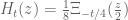 . The original 1950 paper of de Bruijn mentions a function on equation (7.4) which is not given a name, but in our notation would be
  . So it may be that the
  notation first appeared in the work of Csordas et al., but the first appearance of anything resembling this function is by de Bruijn.
20 March, 2018 at 10:54 pm
Anonymous
Perhaps the letter in
in  is because it satisfied the backwards heat equation?
21 March, 2018 at 1:55 pm
not Varga
If the notation was first used in the 1988 paper then we could call it “Csordas’s, Norfolk’s, and Varga’s H-function.” Or we could call it the “Varga H-function” because Varga’s name is shorter and sounds more badass than the names Csordas or Norfolk.
20 March, 2018 at 1:43 pm
Anonymous
Something’s wrong with the typesetting of inequality (6) in the wiki page http://michaelnielsen.org/polymath1/index.php?title=Bounding_the_derivative_of_H_t_-_second_approach. I think it’s missing one or more parentheses and a frac.
[Fixed, thanks – T.]
20 March, 2018 at 3:22 pm
Anonymous
a squared denominator is still missing a left parenthesis
[Corrected, thanks – T.]
20 March, 2018 at 5:21 pm
Anonymous
Is there a version of the derivative-of-Ht bounds (with integral and summation remainder bounds) that uses the original Ht formulation, without the fubini switch of integration and summation and without the theta?
20 March, 2018 at 6:12 pm
Terence Tao
This would basically correspond to setting in the current formulation. One could save a tiny amount in the bound by using the cosine form of the integral, rather than bounding the
  and
and  terms separately and then combining by the triangle inequality.
20 March, 2018 at 5:26 pm
Anonymous
It looks like the active work on this project is happening on the github mailing list and not on the blog.
For example I see “Yeah, one thing we can do is to find the ratio Ht/bound_ddx_Ht and then jump to the furthest point in the fixed mesh which meets the stepsize requirement. That would shorten the verification time. I had run a test of the verification script from x=1000 to 1005 (without jumping), and it around 30 minutes. I now think the ddxbound function (even the non optimized one would do) should also be computed in Arb if possible.”
What is bound_ddx_Ht and what are the fixed mesh and the stepsize requirements? What is the verification script and what does it do? What’s the ddxbound function, and what’s the difference between the optimized and non optimized one?
20 March, 2018 at 10:45 pm
KM
bound_ddx_Ht is the D value in the upper bound of H’t …[D*exp(-theta_c*x)]
Anonymous@Arb had generated data from x=1000 to 1600 using a fixed mesh with stepsize of 0.005, which we have to now use to rigorously prove the non-vanishing of H_t in this x interval. For that we are running a verification script which essentially checks whether 0.005<=allowed step size (which is |H_t/upper bound H't|.
I guess in the process of running numerical exercises, we often come across technical and short term computational challenges. Sometimes they are related to the tools involved, and sometimes of an algorithmic nature, both of which need discussion and collaboration. For example, D turned out to be not that fast to calculate at large scale, so we decided to use the rows from the Arb output in a more optimal way.
21 March, 2018 at 6:51 am
Anonymous
In the main wiki page, “|” is missing before in its explicit (Backlund) estimate.
[Corrected, thanks – T.]
21 March, 2018 at 12:28 pm
Anonymous
The page http://michaelnielsen.org/polymath1/index.php?title=Bounding_the_derivative_of_H_t_-_second_approach has two equations labeled (1). One is for H’t(x) and the other is for theta.
[Renumbered – T.]
22 March, 2018 at 7:48 am
Terence Tao
While working on transcribing the wiki arguments to a LaTeX writeup (you can see the latest draft at https://github.com/km-git-acc/dbn_upper_bound/blob/master/Writeup/debruijn.pdf ) I found that it is slightly more natural to replace the correction term
in the wiki by the minor variant
(using the notation of the wiki). Numerically the two appear to be almost identical once is reasonably large (roughly speaking one is replacing the Gamma function with its Stirling approximation). It is sort of moot right now since we are not using the
  correction, but this might be something of use in the future. Interestingly the phase of
  is very simple, it is just
  (up to sign); this is connected with the
  type decay in the
  direction (as per the Cauchy-Riemann equations), together with the fact that
  is real when
  .
.
23 March, 2018 at 9:10 am
rudolph01
Just an observation that could maybe help speed up future numerical computations.
The following integral expression for :
:
with:
seems to provide a speed boost for direct numerical evaluation in CAS-tools. The additional bonus is that for higher , it doesn’t need increasingly higher precision settings. I guess the speed comes from the optimised evaluation of
  . The strange thing however is that increasing the integral limits above 8 seems to adversely impacts the accuracy.
The following results and timings were obtained with pari/gp:
0.03442027018705231123 – 0.0016782531784355935738*I in 116 ms.
-0.00010001026469315639165 – 7.135701992146987265 E-6*I in 162 ms.
6.702152217279126684 E-16 + 3.133796584070556924 E-16*I in 172 ms
-4.015967420625146363 E-49 – 1.4006524430296850033 E-49*I in 208 ms.
1.4847586783170623283 E-169 + 3.0506306235580557898 E-167*I in 333 ms.
-1.1441895900436789748 E-507 + 1.5701563504659934332 E-507*I in 612 ms.
-5.577340153523143050 E-1701 – 4.087843212390861641 E-1700*I in 1,384 ms.
3.159248518322167576 E-5110 – 6.737020164746385398 E-5110*I in 3,139 ms.
-9.351604489264646152 E-17047 + 4.384024397497349318 E-17047*I in 8,389 ms.
-1.6800823865134499270 E-51156 – 2.434780317427023972 E-51155*I in 21,808 ms.
-9.922871600520644604 E-170537 – 7.584881610937171242 E-170537*I in 1min, 3,987 ms.
Pari/gp code used:
default(realprecision, 40)
xi(s)=(s/2)*(s-1)*Pi^(-s/2)*gamma(s/2)*zeta(s)
Ht(z,t)=1/8*intnum(x=-8,8,xi((1+I*z)/2+sqrt(t)*x)*1/sqrt(Pi)*exp(-x^2))
The numbers exactly match up to 20 digits with the already computed values by user Anonymous. To check the values, I used
  as a proxy. Grateful if someone could confirm by using the ARB libraries how well the fit actually is for these high values.
23 March, 2018 at 9:25 am
Anonymous
Do you have a reference for that integral expression for Ht? I didn’t see it on the wiki.
23 March, 2018 at 9:29 am
rudolph01
It is in the write-up on the wiki that prof. Tao is preparing (see link earlier in this thread).
23 March, 2018 at 9:47 am
Anonymous
I see now, it’s equation (6) in the current version of the pdf. I don’t suppose we have any explicit bounds on the size of the tails of the integral.
23 March, 2018 at 8:44 pm
Terence Tao
I have now written up some tail bounds for these integrals at http://michaelnielsen.org/polymath1/index.php?title=Bounding_the_derivative_of_H_t_-_third_approach . One nice feature of the gaussian integral approach to computing is that one can shift the contour to any horizontal line
  , in particular one can choose a single
  to handle multiple values of
  (though the integrand gets quite oscillatory and large if
  strays too far from
  ). This should be helpful for getting bounds on
  that are uniform for
  in an interval; there may also be some speedup when computing
  for multiple values of
  by first evaluating and storing
  for a fine mesh of
  and then integrating this function against various weights to recover
  .
.
24 March, 2018 at 9:30 am
rudolph01
I tried to code the new Ht and Ht’ formulae as well as their bounds and couldn’t get the numbers properly reconciled. Could there maybe be a mistake (or typo) in the variable change step from defining:
to
Shouldn’t this be:
i.e. also including in the square?
24 March, 2018 at 10:00 am
Terence Tao
Yes, that is a typo, thanks for pointing it out! It propagated a few more lines into the wiki page but I think they are all fixed now.
24 March, 2018 at 11:20 am
KM
In the wiki once xi’s functional eqn is used, the integral and the derivative seem to work if we use xi(1-sigma+iT) instead of taking its conjugate.
[I’ve made this change for now, but I’m not 100% convinced that one can do this – will look at it again tomorrow. -T]
Also some typos in that section. The derivative has a division by t missing in few places, and after the cutoff X is introduced, the second exponential’s numerator should be squared like in other sections.
[Corrected, thanks – T.]
25 March, 2018 at 3:52 am
rudolph01
Two remaining small typo’s in the pieces under “one has” and under “and”.
An additional bonus of these new tail-bounded integrals is that now the evaluation of is just as fast as
  :) When I took the derivative of the original unbounded integral in pari/gp,
  evaluated 4-5 times slower!
[Corrected, thanks – T.]
25 March, 2018 at 4:44 am
KM
Comparing H_t estimates at x=1500,y=t=0.4, we get these values
A+B-C = (3.52-4.63i)*10^-252
Integral from -X to X = similar to A+B-C
Integral from 1/2 to X with xi(sig+iT)*(exp() + exp()) = (3.62+0.14i)*10^-252
Integral from 1/2 to X with xi(sig+iT)*exp() + xi(1-sig+iT)*exp() = similar to A+B-C
Also, possibly a typo in the functional eqn
xi(s)=xi(1-s) -> xi(sig+iT) = xi(1-sig-iT) (currently displayed as xi(1-sig+iT)
[Corrected, thanks – actually the formula was initially correct, but I made it incorrect earlier by misinterpreting a comment on this blog, but hopefully it is now all fixed -T.]
25 March, 2018 at 1:52 pm
rudolph01
With the faster third approach integral now available, I would like to test its performance by rerunning the fixed step mesh (step size ) for
) for  and
and  .
.
For the previous run we have used a list of pre-computed values of (using the ARB library) and the bottleneck of the second integral approach was in evaluating the J-integral to establish the derivative bounds at each x-step.
You already mentioned as a benefit of the third approach, that by choosing T smartly, it might be possible to achieve a single derivative bound for multiple values of (within limits). This will certainly help, but are there maybe other ways to speed up computing the derivative bounds in the third integral approach?
25 March, 2018 at 5:10 pm
Terence Tao
Beyond the trick of fixing T, and using the functional equation to halve the region of integration, I can’t think of any further speedups. One also needs to get upper bounds for the main portion of the derivative integral. The quickest way I know of would be to use the triangle inequality
as this integral has the nice feature that the dependence on is very simple once
  are fixed (it is of the form
  for some numerically computable expressions
  ). I don’t know how well this bound compares with the true derivative, it would be helpful I think to have some numerical results on this.
23 March, 2018 at 10:18 am
Terence Tao
Nice! I didn’t realise that the zeta function was that fast to compute that this integral was numerically feasible. This may well give a different route to fast numerical evaluation of and its derivative with good error estimates, since it is easy to bound
  for say
  (just by using
  ) and then also for
  by the functional equation. If the performance is significantly better than our current approach for the ranges of x we care about (something like
  , I guess) then we could certainly use this as a replacement method. I’ll try to write up some tail bound estimates in the spirit of what we already have on the wiki (and now on the writeup).
24 March, 2018 at 10:52 am
David Bernier (@doubledeckerpot)
This is a lot faster than Anonymous’ Arb code. You mention losing precision when increasing the integration limits. PARI/gp allows to tinker with the integration step in intnum(.), so that with:
Ht(z,t)=1/8*intnum(x=-16,16,xi((1+I*z)/2+sqrt(t)*x)*1/sqrt(Pi)*exp(-x^2), 3)
[ NB, the ‘3’ in argument to intnum means “divide integration step by 8”]
I get this for 1000+ 0.4i:
? Ht(1000+0.4*I, 0.4)
%10 = 1.484758678317062328342109271589162677850 E-169 + 3.050630623558055789723687410028754104648 E-167*I
Arb at 40 digits:
$ ./a.out 0.4 1000 0.4 40
Re[H]: 1.48475867831706232834210927158916267785e-169
Im[H]: 3.050630623558055789723687410028754104648e-167
For x = 100000+0.4*I, it would take probably several hours with Anonymous’ Arb code to compute .
.
24 March, 2018 at 11:29 am
David Bernier (@doubledeckerpot)
For , I used your PARI/gp code with integration limits -16 and 16, and with the integration step divided by 8. This gives the code:
Ht(z,t)=1/8*intnum(x=-16,16,xi((1+I*z)/2+sqrt(t)*x)*1/sqrt(Pi)*exp(-x^2), 3)
and the evaluation:
Ht(1000000+0.4*I, 0.4)
= -9.922871600520644601759753538816405378292 E-170537
– 7.584881610937171236393324520371825126356 E-170537*I
(excellent agreement), in 8 minutes.
24 March, 2018 at 12:39 pm
David Bernier (@doubledeckerpot)
With m=2 instead of m=3, the time is just over 3 minutes for the same integral:
? Ht(z,t)=1/8*intnum(x=-16,16,xi((1+I*z)/2+sqrt(t)*x)*1/sqrt(Pi)*exp(-x^2), 2)
? Ht(1000000+0.4*I, 0.4)
%13 = -9.922871600520644601759753538816405378292 E-170537 – 7.584881610937171236393324520371825126356 E-170537*I
? ##
*** last result computed in 3min, 36,236 ms.
23 March, 2018 at 9:19 am
rudolph01
P.S. whilst copying some latex from the wiki, I spotted that on our “home” wiki page under the header ,
,  should be
  in the definition of
  . In the draft final write-up, it is stated correctly.
[Corrected, thanks – T.]
23 March, 2018 at 10:25 am
Terence Tao
I’m making progress on the writeup at https://github.com/km-git-acc/dbn_upper_bound/blob/master/Writeup/debruijn.pdf . I’ve added a section on using the effective estimates to obtain asymptotic information (without explicit constants) for very large x. Basically, what happens is that for any , the zeroes become very predictable for real part larger than
  for a large absolute constant
  : they become all real, and in fact for each natural number
  there is precisely one real zero of the form
  , where
  solves the equation
This is an increasing sequence that locally looks like an arithmetic progression. (One could in principle solve for explicitly using the Lambert W-function, though the resulting expression is not terribly enlightening.) As time advances, the zeroes all move left with speed close to
  (I recall there were some graphical numerics done previously that confirmed this marching to the left). Furthermore there is a Riemann-von Mangoldt formula: for
  , the number of zeroes of real part between 0 and X is
where now is bounded by an absolute constant. These results strengthen those of Ki-Kim-Lee, which had similar results but where the bounds depended on
  in a non-explicit fashion (and in particular could blow up as
  ).
).
24 March, 2018 at 3:36 pm
rudolph01
Acknowledging that these plots are not in the domain of a large absolute constant , the ‘marching upwards to the left’ of the zeros can already be seen in the lower ranges of
  at higher
  . To test the exact ‘third approach’-integral, I ran the following implicit plots.
One for with
with  varying (I suppressed the imaginary part where numerical error otherwise just shows as noise):
With y=0
And one for with
with  varying. This one nicely reveals where the complex zeros (i.e. the red and green lines cross) of
  are hiding in the area below the line
  :
:
With y=0.4
24 March, 2018 at 7:49 pm
Terence Tao
Thanks for this! And the speed does seem very close to , as predicted by theory.
25 March, 2018 at 2:48 am
Anonymous
Similar results (for zeta nontrivial zeros representation as solutions to a similar equation) appeared in de Reyna and de Lune paper
Click to access 1305.3844.pdf
25 March, 2018 at 3:31 am
Anonymous
The zeros dynamics implies that for each and
and  , the zeros
  (horizontal) velocities should be
  , but since these velocities are in fact bounded (close to
  ), it seems that (due to the regularity of the distribution of
  ) the infinite sum representing
  (horizontal) velocity should have a lot of cancellation (e.g. similar to cancellations in singular integrals) – which makes it bounded.
25 March, 2018 at 7:12 am
Terence Tao
Yes, in fact as the zeroes are so evenly spaced, the net force of nearby zeroes is negligible (something like ). The
  drift is instead coming from a long-distance effect: there are somewhat fewer zeroes about
  units to the left of
  then there are
  units to the right of
  , because the zeroes get denser as one moves away from the origin. The
  additional zeroes to the right are ultimately the main source of the
  velocity to the left. (One would get a similar phenomenon if one forgot about the zeta function entirely and applied heat flow to
  (i.e. the
  main term in the Riemann-Siegel formula) instead of
  .)
.)
23 March, 2018 at 12:05 pm
Anonymous
Is it possible that by including the refinement in the asymptotic approximation, the threshold
  may be improved?
23 March, 2018 at 3:18 pm
Terence Tao
Actually, the error is not the dominant term that causes the problem. It’s more to do with the tail of
  , or in the toy model
  . In order to get good control on the zeroes, one needs the
  term to dominate all the others, and this only happens when
  is large, that is if
  (note that for the purpose of locating zeroes one would mostly be interested in the
  case). Below this range, one expects all the
  summands to interact with each other in a nontrivial way, giving the same sort of complex behaviour one sees in the Riemann zeta function, where the slowly converging nature of
  gives rise to oscillations on the critical line
  that are still only poorly understood. (The
  term is comparable in strength to the last term
  in this sum; not entirely negligible, but still fairly small compared to the net contribution of the other summands.)
23 March, 2018 at 7:45 pm
Anonymous
I think there’s a typo in the definition of in the new wiki page, where
  should be
  .
.
[Corrected, thanks – T.]
23 March, 2018 at 9:22 pm
Anonymous
on the wiki a few lines below (3) a bound on abs(xi(s)) is written as an equation but it should be an inequality.
the inequality above (3) is missing one vertical bar
[Corrected, thanks – T.]
23 March, 2018 at 10:49 pm
Anonymous
Here’s some output of an adaptive mesh script based on the “second approach” derivative bounds wiki page, for t=0.4, x between 20 and 1000, y=0.4, digits=20.
https://gist.githubusercontent.com/p15-git-acc/3ada0ff0b9ec77e23cb7cace0dcb8691/raw/807e1b0a16356a9bbd2a5af872f71bc064830c38/gistfile1.txt
It took 3 or 4 hours to run. The “D” and “step” values should mean the same thing as in https://terrytao.wordpress.com/2018/03/02/polymath15-fifth-thread-finishing-off-the-test-problem/#comment-494166. The output should have full accuracy, not just for the H values but also for the “D” and “step” values.
If I understand correctly, other people have already covered this range of x, and furthermore the method I used is about to become obsolete due to the “third approach” for derivative bounds. For those reasons I haven’t yet spent any time turning the code into a single file that other people could build and run.
24 March, 2018 at 8:03 am
KM
I think any speedup seen with other libraries would be even more pronounced with a library like Arb. Moreover, it would be great to see how you wrote the adaptive mesh, so please share your scripts if possible.
24 March, 2018 at 8:11 am
K
I have a non-expert question for the numerics-team: On which computer systems are you running your code? Is it parallelized? Can it use the GPU? Thanks for participating in this exciting project!
24 March, 2018 at 9:07 am
Anonymous
As far as I know no one is using GPU, and parallelization is limited to running a few (like 2) instances of the same script on different ranges of x on the same computer. Different people are using different systems (windows, mac, linux). The use of github for version control has temporarily stagnated and it’s currently being used as a mailing list where people post new versions of their code as attachments to comments in a single issue thread.
25 March, 2018 at 9:11 am
K
Is it possible to specify an upper bound for , which can not be overcome with the methods available today? Similar to the Prime Gap Conjecture, where the Bound
  is the best (assuming the generalized EH conjecture) – due to the parity problem for sieve methods. Did you identify any “no-go” problem in this project?
25 March, 2018 at 1:49 pm
Anonymous
There’s a typo in one of the lines between (1) and (2) in http://michaelnielsen.org/polymath1/index.php?title=Bounding_the_derivative_of_H_t_-_third_approach where a conj(xi(sigma + i*T)) has gone missing.
25 March, 2018 at 3:27 pm
Anonymous
Updated C code (needs the arb library from arblib.org) to compute H or its derivative, implementing the third approach for derivative bounds:
https://pastebin.com/1uk3V6CP
./a.out 0.4 100 0.4 1 20
Re: 7.8282744022553779399e-16
Im: -2.537161602132201872e-16
time ./a.out 0.4 1e6 0.4 0 20
Re: -9.9228716005206446018e-170537
Im: -7.5848816109371712364e-170537
real 0m0.999s
user 0m0.996s
sys 0m0.004s
25 March, 2018 at 5:01 pm
Terence Tao
Is your first calculation an evaluation of ? It seems to differ from other evaluations of this quantity (which are roughly
  ). If you are using the formulae on the wiki, there was an issue with some of the integrals not having the complex conjugate term
  applied correctly, which has hopefully now been fixed.
25 March, 2018 at 5:05 pm
Anonymous
Sorry, the first one is an evaluation of the derivative. The help string for the program is
—
Usage:
./a.out t x y n d
Evaluate the nth derivative of H_t(x + yi) to d significant digits where H is the function involved in the definition of the De Bruijn-Newman constant.
Requires x >= 0 and y >= 0 and t <= 1/2 and n in {0, 1}.
—
so for
./a.out 0.4 100 0.4 1 20
this means
t=0.4 x=100 y=0.4 derivative=1 digits=20
The output can be compared to what Rudolph found using PARI/GP in https://github.com/km-git-acc/dbn_upper_bound/issues/50#issuecomment-375984748
25 March, 2018 at 5:36 pm
Terence Tao
Ah OK, thanks for clarifying. Good to see that all the numerics are in agreement :)
26 March, 2018 at 1:45 am
rudolph01
Thanks, Anonymous. Do I read it correctly that your new ARB/C-code completed x=1,000,000 in less than a second? If so, that would be a stunning result and is a factor 60 (!) faster than the third approach in pari/gp. What kind of hardware are you running on? Could you maybe share some more timed results for e.g. in steps x=10^k?
26 March, 2018 at 3:42 am
Anonymous
Yes Rudolph your idea to use zeta directly is pretty fast! Here’s what I have for x up to 1e10 in powers of 10, running on one core of a normal desktop computer that is about as fast as David’s.
./a.out 0.4 1 0.4 0 20
Re: 0.062123742002240553423
Im: -0.00028956980995331115603
0.168s
./a.out 0.4 10 0.4 0 20
Re: 0.034420270187052311229
Im: -0.0016782531784355935738
0.039s
./a.out 0.4 100 0.4 0 20
Re: 6.7021522172791266841e-16
Im: 3.1337965840705569244e-16
0.057s
./a.out 0.4 1000 0.4 0 20
Re: 1.4847586783170623283e-169
Im: 3.0506306235580557897e-167
0.133s
./a.out 0.4 1e4 0.4 0 20
Re: -5.5773401535231430494e-1701
Im: -4.0878432123908616412e-1700
0.427s
./a.out 0.4 1e5 0.4 0 20
Re: -9.3516044892646461514e-17047
Im: 4.3840243974973493177e-17047
1.997s
./a.out 0.4 1e6 0.4 0 20
Re: -9.9228716005206446018e-170537
Im: -7.5848816109371712364e-170537
0.950s
./a.out 0.4 1e7 0.4 0 20
Re: 4.6135825683593727239e-1705458
Im: -1.4529659713176507443e-1705457
1.297s
./a.out 0.4 1e8 0.4 0 20
Re: -5.8234400633053449049e-17054689
Im: -6.4741134049720791141e-17054690
1.837s
./a.out 0.4 1e9 0.4 0 20
Re: -2.556450161624682077e-170547026
Im: 2.9149196815349427501e-170547026
4.856s
./a.out 0.4 1e10 0.4 0 20
Re: 1.500919785954441619e-1705470421
Im: 7.8891699583970818103e-1705470423
15.911s
26 March, 2018 at 3:59 am
rudolph01
Amazing! Only 8 days ago we were complaining about taking 13 minutes to compute at 5 digits only and now we do
  in only 16 seconds at 20 digits on a home PC…
If we continue this way, the exact value of will be computed faster than its approximation :)
P.S.: seems slower than
  . Also the timing for
  looks a bit odd. Are these correct?
25 March, 2018 at 6:00 pm
Terence Tao
I’d like to mention here that one of the early approaches to bounding may end up being more numerically viable as we go below 0.48. Right now we are relying on the following criterion:
Criterion 1: If whenever
  , then
  .
.
Verifying this criterion requires a lengthy mesh evaluation of either or an approximant
  which seems to be the computational bottleneck. On the other hand, we have a slightly different criterion from http://michaelnielsen.org/polymath1/index.php?title=Dynamics_of_zeros :
Criterion 2: If
All the zeroes of with
with  are real;
 whenever
  ,
,  , and
, and  ; (one can also shrink this region a bit, see wiki) and
 whenever
  and
and  ,
,
then .
.
Because of extensive numerical verification of RH, the first condition will basically be automatic for any we would reasonably consider using. Probably one would pick
  so that the third condition can be verified analytically (much as we are already doing for
  at around
  , so
, so  ).
). (or
(or  ) for
) for  in a short interval
 ![[X,X+1]](https://s0.wp.com/latex.php?latex=%5BX%2CX%2B1%5D&bg=ffffff&fg=545454&s=0&c=20201002) rather than a long interval
rather than a long interval ![[0,X]](https://s0.wp.com/latex.php?latex=%5B0%2CX%5D&bg=ffffff&fg=545454&s=0&c=20201002) . However, the drawback is that one has to do this for all
. However, the drawback is that one has to do this for all  rather at just
  , so we will also need derivative estimates in the t aspect. The main issue here is that I think the derivative begins to deteriorate as
  (or more relevantly, the rigorous upper bounds on the derivative deteriorate). However, it may still be a net computational win, and maybe something to explore as we go beyond 0.48.
The potential win here is that we only need to numerically evaluate
26 March, 2018 at 12:26 am
Anonymous
A possible idea to bound the horizontal velocity of a (hypothetical) nonreal zero of is to represent it as a sum of the real zeros contribution (which may be bounded – using the cancellation in its representing sum) and the contribution due to other (hypothetical) nonreal zeros of
  (which may be bounded by using known estimates on the horizontal distribution of hypothetical “very rare” nonreal zeros of
  with
with  and the contribution due to nonreal zeros with
  is similar and may be absorbed by the contribution of the real zeros.)
 (hence also of
  ) with
  .
.
The main idea here is to exploit also the known information on the horizontal distribution of “very rare” nonreal zeros of
26 March, 2018 at 2:22 am
Anonymous
Is it possible (for fixed ) to use a 2D mesh with (adaptive) steps in both
  and
and  intervals?
 should be chosen near the middle of a relatively large gap between two consecutive zeros of
  .
.
It seems that
26 March, 2018 at 3:18 am
Anonymous
It seems that the second condition in criterion 2, with varying and varying
  in a short interval
  can be simplified by verifying it only for
  at the end points
  of the interval (to prevent from any nonreal zero to enter the interval while
  is increasing from
  to
to  ).
). and 2D mesh in both
  and
and  (instead of 3D mesh in
  ).
).  should be chosen with relatively large distances from the (nearest) zeros of
  .
.
Therefore it seems sufficient to use fixed
25 March, 2018 at 10:01 pm
Anonymous
Does http://michaelnielsen.org/polymath1/index.php?title=Bounding_the_derivative_of_H_t_-_second_approach have any limitations on x other than inequality (2) and the analogous inequality where X=0? Can the formulas on that page be used to evaluate Ht and to bound its derivative when x is near zero?
26 March, 2018 at 7:21 am
Terence Tao
Yes, that is one key advantage of this second approach. In contrast, the third approach technically works for x near zero, but the error term degrades because the parameter , which prefers to be close to
  , is constrained to be at least 1. This is mainly due to the breakdown of the Stirling approximation to the gamma function near the negative real axis (where the poles are). In principle one could tighten the third approach to give better results for very small
  (since by the functional equation we only need to evaluate xi on the right half-plane and so the negative real axis should not be an issue), but this looks like a region which is well controlled in any case, so this is presumably not a priority.
26 March, 2018 at 10:07 am
Anonymous
I have a question that I want to call super naive except I that don’t want to discourage other readers of the blog from asking stupid questions too. When we accumulate certain evaluations of functions of endpoints of intervals on a mesh along a directed perimeter of a rectangle in the complex plane in order to count the zeros inside the rectangle, I understand how the derivative bound in http://michaelnielsen.org/polymath1/index.php?title=Bounding_the_derivative_of_H_t_-_second_approach helps us to determine the mesh granularity along the horizontal lines where y is constant and x varies, but I don’t understand how we determine the granularity along the vertical lines when y varies and x is constant. Is there a monotonicity property that we use? This question is for x < 2000.
26 March, 2018 at 11:30 am
Terence Tao
The function is holomorphic, so we have the Cauchy-Riemann equations
  , so the derivative bound controls both horizontal and vertical variation. Similarly for
  , which is also holomorphic.
26 March, 2018 at 11:46 am
Anonymous
The derivative bound controls both horizontal and vertical variation, but does it control variation on the whole interval between vertical mesh points or only between horizontal mesh points? For the horizontal mesh there’s a statement about the bound “After fixing n0, X, theta, the only x dependence in these terms is a factor of exp(-theta*x), so one gets uniform estimates for any x >= x0.” Is there an analogous uniform estimate for any y >= y0, or do we not need one, or is it obvious from the uniform estimate for x?
26 March, 2018 at 12:53 pm
Terence Tao
Good point! Fortunately only enters through the parameter
  (which is set equal to the four values of
  ) and the bounds are monotone increasing in
  (as can be seen from inspection of the integrals). So for the
  terms one would need to substitute the upper bound on
  , while for
  one would need the lower bound on
  .
.
Alternatively, we can avoid all use of vertical line segments and work with an enormous rectangle where
where  is much larger than
  . When sending
  infinity, the analytic estimates ensure that the variation on the far right edge is asymptotically negligible, and analytic estimates should also be able to handle the variation between
  and
and  . The segments
  and
and  (as well as the easy vertical line segment
  ) would still have to be done numerically, of course.
26 March, 2018 at 1:34 pm
Terence Tao
We have two basic approaches right now to prevent zeroes of from entering the region
  . Our primary approach is to directly use the argument principle, evaluating
  either exactly or approximately at
  (and also at a higher horizontal line). In a previous comment I also mentioned a secondary approach in which the main task is to block out zeroes instead in a region
  but now for all
  .
.
There is a third approach that I had previously discounted but am now rethinking, which is to start with the fact that the zeroes of are already known to be real up to a very large value
  of
of  (something like
  ) due to the existing numerical work on RH, and try to prevent all the non-real zeroes from moving down into smaller values of x as
  increases. If for instance one can show that by time
  there are still no non-real zeroes with
  and
and  , then by combining this with our analytic results we can certify the entire region
  as free of zeroes of
  without doing any further numerics in the
  region. (Note that while non-real zeroes can (and eventually will) collide with their complex conjugate to become real, the converse cannot happen: zeroes that are real stay real forever.)
The problem I had been facing with this third approach was that there was no upper bound on the horizontal velocity of zeroes, particularly in the “big bang” period when is very close to zero. If there were two adjacent zeroes that were aligned to be almost horizontal to each other, then the one on the left will fly leftwards with a huge negative velocity. In principle, this might mean that one or more complex zeroes that were just outside the range
  of numerical verification at time
  could zoom into the bad zone
  in an arbitrarily small amount of time (unless there is some barrier to stop this, such as the one erected in the second approach).
However, what I now realise is that whenever this occurs, the other zero in the pair of nearby zeroes will acquire an equal and opposite large velocity to the right. So if one works with some sort of aggregate statistic that sums over all zeroes, rather than focusing on the dynamics of a single zero, then things appears to be much better behaved.
I am starting to work out what happens in particular to the statistic
which is a weighted sum of zeroes above the real axis. At time 0 it should be possible to ensure that this expression is quite small for reasonably large X, e.g. . The derivative to this expression contains a lot of terms, one for each pair of zeroes, but the pairs that are far from each other (distance
  , say) seem to contribute
  or better (plus some negligible errors), and the pairs that are close to each other seem to be contributing something like
  (using some Riemann von Mangoldt formulae that I have just added to the asymptotics section of the writeup that stay uniform as t approaches 0). So it looks like Gronwall’s inequality is going to keep this statistic small for later times such as
  which should hopefully be enough to prevent zeroes high above the real axis.
In order for this to work properly one needs effective Riemann von Mangoldt formulae on the number of zeroes of of real part up to any given
  . This could be a bit messy. On the other hand it looks like error terms are something like
  of the main term which is very promising and could allow for a fair amount of slack in the effective estimates. Anyway I will try to work out something more precise on this possible third approach.
26 March, 2018 at 10:47 pm
Anonymous
Since the terms in the sum for
  vanish for
  , the restriction
  in the sum may be relaxed to
  (which does not distinguish between real zeros and zeros with
  .) To deal simultaneously also with the
  case, one may replace the factor
  by its absolute value
  , but it seems better to replace it by
  (since the zeros vertical dynamics for
  is more regular for small
  than that of
  or
or  .) The statistic
  can also be made more flexible by replacing
  (in the exponent) by
  .
.
Therefore, my suggestion is to modify the terms in the sum for by
by  , where the (unrestricted!) sum is over all the zeros
  of
of  and the scaling factor
  may depend on
  .
.
27 March, 2018 at 12:28 am
Anonymous
A more systematic (and flexible) approach is to use the general statistic
For sufficiently smooth weight function over the complex plane, with some desirable properties (e.g.
  – to avoid contribution from the real zeros of
  ) such that by using information on the asymptotic distribution and dynamics of
  zeros, there is a sufficiently good estimate (or even a “main term”) with effective error bounds for the (time) derivative of the statistic
  .
. .
.
This approach (similar to the approach in Polymath8) seems to lead to a variational optimization problem for the weight function
27 March, 2018 at 5:48 pm
Terence Tao
This is certainly a possibility; in particular it seems beneficial to truncate the weight to be compactly supported. But this particular choice of weight seems to have relatively good properties, in particular I wrote up some asymptotic calculations at http://michaelnielsen.org/polymath1/index.php?title=Dynamics_of_zeros#Derivative_analysis that indicate that the quantity
  grows quite slowly in time.
28 March, 2018 at 12:24 am
Anonymous
The time derivatives of zeros and the statistic
  are well defined except for (at most countably many) “singular” t-values for which
  has a multiple zero. Since for any fixed
  there are at most finitely many non-real zeros of
  for each
  , it follows that there are only finitely many “singular” t-values in
  , implying that
  is continuous and piecewise smooth on
  (it might not be differentiable only for such “singular” t-values).
 should apply for each open interval between consecutive singular t-values, and by continuity they should apply (for each fixed
  ) for all
  but in terms of
  (still not in terms of
  !).
!). at
at  , we see that by letting
  , the estimate of
  via
via  tends to the desired estimate of
  in terms of
  .
.
Therefore the above estimates of
Now by using the continuity of
28 March, 2018 at 10:43 am
Anonymous
Can this approach (using the weighted sum statistic over zeros) be interpreted as a kind of sieve method (for
  zeros – similar to the usual sieve methods for primes)?
26 March, 2018 at 6:05 pm
Anonymous
Is the test problem finished, or finished enough to have served its purpose?
27 March, 2018 at 5:47 pm
Terence Tao
I’ll defer to the numerics team for the precise status, but I think we have cleared all but the fairly small values of (maybe something like
  ) for the toy problem, but should soon have the capability to do that also. The same methods, with a little bit more work (basically requiring one to analyse y=0.45 as well as 0.4) should then soon give the bound
  . Once we figure out how to do that it should be relatively easy to see how far the methods can be pushed, by testing various ways in which to lower the
  and
and  parameters. (Presumably one does not need to do a full mesh evaluation etc. for these parameters to get a rough sense of whether the method is feasible there.)
27 March, 2018 at 8:33 pm
KM
I think everything except the x lte 1000, y=0.45 line segment (and the other two smaller sides of the rectangle) is covered. With the latest estimates on the (A+B) error bounds, we may in fact require to verify this segment only for N lte 6. We are running it now for the entire rectangle with the third integral approach.
Using the first and second integral approaches, the x lte 1600,y=0.4 part had been verified earlier (mentioned in these fifth thread comments 1000 lte x lte 1600 and x lt 1000).
27 March, 2018 at 8:57 pm
Anonymous
Here’s a script that counts roots of inside the region where
  and
and  using the argument principle and Rouché's theorem. It is designed to be exact, using interval arithmetic and explicit tail bounds everywhere. On the other hand it is slow and it might not terminate for inputs that are much different from the examples below.
Most of the formulas are taken from http://michaelnielsen.org/polymath1/index.php?title=Bounding_the_derivative_of_H_t_-_second_approach .
Source code: https://pastebin.com/TiFk6CfF
—
./a.out t xa xb ya yb
Count the roots of H_t(x + yi).
xa < x < xb
ya < y < yb
—
./a.out 0 50 70 -1 2
3
0m13.731s
./a.out 0.4 50 70 -1 2
2
0m11.459s
./a.out 0.4 0 100 0.4 0.45
0
1m9.112s
./a.out 0.4 100 200 0.4 0.45
0
5m27.415s
./a.out 0.4 200 300 0.4 0.45
0
10m12.504s
28 March, 2018 at 3:44 am
Anonymous
For what it’s worth I also have
./a.out 0.4 300 1000 0.4 0.45
0
266m51.174s
28 March, 2018 at 8:41 am
KM
Amazing. With your last four estimates, I guess all the pieces are in place and the ‘jigsaw’ is complete :)
28 March, 2018 at 12:54 pm
Terence Tao
Looks like a good time to roll over to a new thread then, since we’ve hit 100 comments in any case. Will do that now.
31 March, 2018 at 12:00 pm
KM
@Anonymous, to make it easier to find your scripts, I have created a Arb folder in the repo where the three pastebin links are documented.
28 March, 2018 at 1:14 pm
Polymath15, seventh thread: going below 0.48 | What's new
[…] thread of the Polymath15 project to upper bound the de Bruijn-Newman constant , continuing this post. Discussion of the project of a non-research nature can continue for now in the existing proposal […]