254A, Notes 1: Local well-posedness of the Navier-Stokes equations

We now begin the rigorous theory of the incompressible Navier-Stokes equations

where is a given constant (the kinematic viscosity, or viscosity for short), is an unknown vector field (the velocity field), and is an unknown scalar field (the pressure field). Here is a time interval, usually of the form or . We will either be interested in spatially decaying situations, in which decays to zero as , or -periodic (or periodic for short) settings, in which one has for all . (One can also require the pressure to be periodic as well; this brings up a small subtlety in the uniqueness theory for these equations, which we will address later in this set of notes.) As is usual, we abuse notation by identifying a -periodic function on with a function on the torus .

In order for the system (1) to even make sense, one requires some level of regularity on the unknown fields ; this turns out to be a relatively important technical issue that will require some attention later in this set of notes, and we will end up transforming (1) into other forms that are more suitable for lower regularity candidate solution. Our focus here will be on local existence of these solutions in a short time interval or , for some . (One could in principle also consider solutions that extend to negative times, but it turns out that the equations are not time-reversible, and the forward evolution is significantly more natural to study than the backwards one.) The study of Euler equations, in which , will be deferred to subsequent lecture notes.

As the unknown fields involve a time parameter , and the first equation of (1) involves time derivatives of , the system (1) should be viewed as describing an evolution for the velocity field . (As we shall see later, the pressure is not really an independent dynamical field, as it can essentially be expressed in terms of the velocity field without requiring any differentiation or integration in time.) As such, the natural question to study for this system is the initial value problem, in which an initial velocity field is specified, and one wishes to locate a solution to the system (1) with initial condition

for . Of course, in order for this initial condition to be compatible with the second equation in (1), we need the compatibility condition

and one should also impose some regularity, decay, and/or periodicity hypotheses on in order to be compatible with corresponding level of regularity etc. on the solution .

The fundamental questions in the local theory of an evolution equation are that of existence, uniqueness, and continuous dependence. In the context of the Navier-Stokes equations, these questions can be phrased (somewhat broadly) as follows:

• (a) (Local existence) Given suitable initial data , does there exist a solution to the above initial value problem that exists for some time ? What can one say about the time of existence? How regular is the solution?
• (b) (Uniqueness) Is it possible to have two solutions of a certain regularity class to the same initial value problem on a common time interval ? To what extent does the answer to this question depend on the regularity assumed on one or both of the solutions? Does one need to normalise the solutions beforehand in order to obtain uniqueness?
• (c) (Continuous dependence on data) If one perturbs the initial conditions by a small amount, what happens to the solution and on the time of existence ? (This question tends to only be sensible once one has a reasonable uniqueness theory.)

The answers to these questions tend to be more complicated than a simple “Yes” or “No”, for instance they can depend on the precise regularity hypotheses one wishes to impose on the data and on the solution, and even on exactly how one interprets the concept of a “solution”. However, once one settles on such a set of hypotheses, it generally happens that one either gets a “strong” theory (in which one has existence, uniqueness, and continuous dependence on the data), a “weak” theory (in which one has existence of somewhat low-quality solutions, but with only limited uniqueness results (or even some spectacular failures of uniqueness) and almost no continuous dependence on data), or no satsfactory theory whatsoever. In the former case, we say (roughly speaking) that the initial value problem is locally well-posed, and one can then try to build upon the theory to explore more interesting topics such as global existence and asymptotics, classifying potential blowup, rigorous justification of conservation laws, and so forth. With a weak local theory, it becomes much more difficult to address these latter sorts of questions, and there are serious analytic pitfalls that one could fall into if one tries too strenuously to treat weak solutions as if they were strong. (For instance, conservation laws that are rigorously justified for strong, high-regularity solutions may well fail for weak, low-regularity ones.) Also, even if one is primarily interested in solutions at one level of regularity, the well-posedness theory at another level of regularity can be very helpful; for instance, if one is interested in smooth solutions in , it turns out that the well-posedness theory at the critical regularity of can be used to establish globally smooth solutions from small initial data. As such, it can become quite important to know what kind of local theory one can obtain for a given equation.

This set of notes will focus on the “strong” theory, in which a substantial amount of regularity is assumed in the initial data and solution, giving a satisfactory (albeit largely local-in-time) well-posedness theory. “Weak” solutions will be considered in later notes.

The Navier-Stokes equations are not the simplest of partial differential equations to study, in part because they are an amalgam of three more basic equations, which behave rather differently from each other (for instance the first equation is nonlinear, while the latter two are linear):

• (a) Transport equations such as .
• (b) Diffusion equations (or heat equations) such as .
• (c) Systems such as , , which (for want of a better name) we will call Leray systems.

Accordingly, we will devote some time to getting some preliminary understanding of the linear diffusion and Leray systems before returning to the theory for the Navier-Stokes equation. Transport systems will be discussed further in subsequent notes; in this set of notes, we will instead focus on a more basic example of nonlinear equations, namely the first-order ordinary differential equation

where takes values in some finite-dimensional (real or complex) vector space on some time interval , and is a given linear or nonlinear function. (Here, we use “interval” to denote a connected non-empty subset of ; in particular, we allow intervals to be half-infinite or infinite, or to be open, closed, or half-open.) Fundamental results in this area include the Picard existence and uniqueness theorem, the Duhamel formula, and Grönwall’s inequality; they will serve as motivation for the approach to local well-posedness that we will adopt in this set of notes. (There are other ways to construct strong or weak solutions for Navier-Stokes and Euler equations, which we will discuss in later notes.)

A key role in our treatment here will be played by the fundamental theorem of calculus (in various forms and variations). Roughly speaking, this theorem, and its variants, allow us to recast differential equations (such as (1) or (4)) as integral equations. Such integral equations are less tractable algebraically than their differential counterparts (for instance, they are not ideal for verifying conservation laws), but are significantly more convenient for well-posedness theory, basically because integration tends to increase the regularity of a function, while differentiation reduces it. (Indeed, the problem of “losing derivatives”, or more precisely “losing regularity”, is a key obstacle that one often has to address when trying to establish well-posedness for PDE, particularly those that are quite nonlinear and with rough initial data, though for nonlinear parabolic equations such as Navier-Stokes the obstacle is not as serious as it is for some other PDE, due to the smoothing effects of the heat equation.)

One weakness of the methods deployed here are that the quantitative bounds produced deteriorate to the point of uselessness in the inviscid limit , rendering these techniques unsuitable for analysing the Euler equations in which . However, some of the methods developed in later notes have bounds that remain uniform in the limit, allowing one to also treat the Euler equations.

In this and subsequent set of notes, we use the following asymptotic notation (a variant of Vinogradov notation that is commonly used in PDE and harmonic analysis). The statement , , or will be used to denote an estimate of the form (or equivalently ) for some constant , and will be used to denote the estimates . If the constant depends on other parameters (such as the dimension ), this will be indicated by subscripts, thus for instance denotes the estimate for some depending on .

— 1. Ordinary differential equations —

We now study solutions to ordinary differential equations (4), focusing in particular on the initial value problem when the initial state is specified. We restrict attention to strong solutions , in which is continuously differentiable () in the time variable, so that the derivative in (4) can be interpreted as the classical (strong) derivative, and one has the classical fundamental theorem of calculus

whenever (in this post we use the signed definite integral, thus ).

We begin with homogeneous linear equations

where is a linear operator. Using the integrating factor , where is the matrix exponential of , and noting that , we see that this equation is equivalent to

and hence from the fundamental theorem of calculus we see that if then we have the unique global solution , or equivalently

More generally, if one wishes to solve the inhomogeneous linear equation

for some continuous with initial condition , then from the fundamental theorem of calculus we have a unique global solution given by

or equivalently one has the Duhamel’s formula

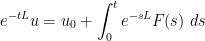
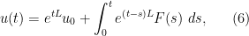
which is continuously differentiable in time if is continuous. Intuitively, the first term represents the contribution of the initial data to the solution at time (with the factor representing the evolution from time to time ), while the integrand represents the contribution of the forcing term at time to the solution at time (with the factor representing the evolution from time to time ).

One can apply a similar analysis to the differential inequality

where is now a scalar continuously differentiable function, are continuous functions, and is an interval containing as its left endpoint; we also assume an initial condition . Here, the natural integrating factor is 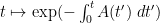, whose derivative is 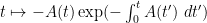by the chain rule and the fundamental theorem of calculus. Applying this integrating factor to (7), we may write it as

and hence by the fundamental theorem of calculus we have

or equivalently

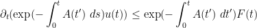
for all (compare with (6)). This is the differential form of Grönwall’s inequality. In the homogeneous case , the inequality of course simplifies to

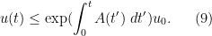
We continue assuming that for simplicity. From the fundamental theorem of calculus, (7) (and the initial condition ) implies the integral inequality

although the converse implication of (7) from (10) is false in general. Nevertheless, there is an analogue of (9) just assuming the weaker inequality (10), and not requiring any differentiability on , at least when all functions involved are non-negative:

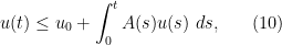
Lemma 1 (Integral form of Grönwall inequality) Let be an interval containing as left endpoint, let , and let , be continuous functions obeying the inequality (10) for all . Then one has (9) for all .

Proof: From (10) and the fundamental theorem of calculus, the function is continuously differentiable and obeys the differential inequality

(note here that we use the hypothesis that is non-negative). Applying the differential form (9) of Gronwall’s inequality, we conclude that

The claim now follows from (10).

Exercise 2 Relax the hypotheses of continuity on to that of being measurable and bounded on compact intervals. (You will need tools such as the fundamental theorem of calculus for absolutely continuous or Lipschitz functions, covered for instance in this previous set of notes.)

Gronwall’s inequality is an excellent tool for bounding the growth of a solution to an ODE or PDE, or the difference between two such solutions. Here is a basic example, one half of the Picard (or Picard-Lindeöf) theorem:

Theorem 3 (Picard uniqueness theorem) Let be an interval, let be a finite-dimensional vector space, let be a function that is Lipschitz continuous on every bounded subset of , and let be continuously differentiable solutions to the ODE (4), thus

on . If for some , then and agree identically on , thus for all .

Proof: By translating and we may assume without loss of generality that . By splitting into at most two intervals, we may assume that is either the left or right endpoint of ; by applying the time reversal symmetry of replacing by respectively, and also replacing by and , we may assume without loss of generality that is the left endpoint of . Finally, by writing as the union of compact intervals with left endpoint , we may assume without loss of generality that is compact. In particular, are bounded and hence is Lipschitz continuous with some finite Lipschitz constant on the ranges of and .

From the fundamental theorem of calculus we have

and

for every ; subtracting, we conclude

Applying the Lipschitz property of and the triangle inequality, we conclude that

By the integral form of Grönwall’s inequality, we conclude that

and the claim follows.

Remark 4 The same result applies for infinite-dimensional normed vector spaces , at least if one requires to be continuously differentiable in the strong (Fréchet) sense; the proof is identical.

Exercise 5 (Comparison principle) Let be a function that is Lipschitz continuous on compact intervals. Let be an interval, and let be continuously differentiable functions such that

and

for all .

• (a) Suppose that for some . Show that for all with . (Hint: there are several ways to proceed here. One is to try to verify the hypotheses of Grönwall’s inequality for the quantity or .)
• (b) Suppose that for some . Show that for all with .

Now we turn to the existence side of the Picard theorem.

Theorem 6 (Picard existence theorem) Let be a finite dimensional normed vector space, let , and let lie in the closed ball . Let be a function which has a Lipschitz constant of on the ball . If one sets

then there exists a continuously differentiable solution to the ODE (4) with initial data such that for all .

Note that the solution produced by this theorem is unique on , thanks to Theorem 3. We will be primarily concerned with the case , in which case the time of existence simplifies to .

Proof: Using the fundamental theorem of calculus, we write (4) (with initial condition ) in integral form as

Indeed, if is continuously differentiable and solves (4) with on , then (12) holds on . Conversely, if is continuous and solves (12) on , then by the fundamental theorem of calculus the right-hand side of (12) (and hence ) is continuously differentiable and solves (4) with . Thus it suffices to solve the integral equation (12) with a solution taking values in .

We can view this as a fixed point problem. Let denote the space of continuous functions from to . We give this the uniform metric

As is well known, becomes a complete metric space with this metric. Let denote the map

Let us first verify that does map to . If , then is clearly continuous. For any , one has from the triangle inequality that

by choice of , hence as claimed. A similar argument shows that is in fact a contraction on . Namely, if , then

and hence by choice of . Applying the contraction mapping theorem, we obtain a fixed point to the equation , which is precisely (12), and the claim follows.

Remark 7 The proof extends without difficulty to infinite dimensional Banach spaces . Up to a multiplicative constant, the result is sharp. For instance, consider the linear ODE for some , with . Here, the function is of course Lipschitz with constant on all of , and the solution is of the form , hence will exit in time , which is only larger than the time given by the above theorem by a multiplicative constant.

We can iterate the Picard existence theorem (and combine it with the uniqueness theorem) to conclude that there is a maximal Cauchy development to the ODE (4) with initial data , with the solution diverging to infinity (or “blowing up”) at the endpoint if this endpoint is finite, and similarly for (thus one has a dichotomy between global existence and finite time blowup). More precisely:

Theorem 8 (Maximal Cauchy development) Let be a finite dimensional normed vector space, let , and let be a function which is Lipschitz on bounded sets. Then there exists and a continuously differentiable solution to (4) with , such that if is finite, and if is finite. Furthermore, , and are unique.

Proof: Uniqueness follows easily from Theorem 3. For existence, let be the union of all the intervals containing for which there is a continuously differentiable solution to (4) with . From Theorem 6 contains a neighbourhood of the origin. From Theorem 3 one can glue all the solutions together to obtain a continuously differentiable solution to (4) with . If is contained in , then by Theorem 6 (and time translation) one could find a solution to (4) in a neighbourhood of such that ; by Theorem 3 we must then have , otherwise we could glue to and obtain a solution on a larger domain than , contradicting the definition of . Thus is open, and is of the form for some .

Suppose for contradiction that is finite and does not go to infinity as . Then there exists a finite and a sequence such that . Let be the Lipschitz constant of on . By Theorem 6, for each one can find a solution to (4) on with , where does not depend on . For large enough, this and Theorem 6 allow us to extend the solution outside of , contradicting the definition of . Thus we have when is finite, and a similar argument gives when is finite.

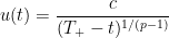
Remark 9 Theorem 6 gives a more quantitative description of the blowup: if is finite, then for any , one must have

where is the Lipschitz constant of on . This can be used to give some explicit lower bound on blowup rates. For instance, if and behaves like for some in the sense that the Lipschitz constant of on is for any , then we obtain a lower bound

as , if is finite, and similarly when is finite. This type of blowup rate is sharp. For instance, consider the scalar ODE

where takes values in and is fixed. Then for any , one has explicit solutions on of the form

where is a positive constant depending only on . The blowup rate at is consistent with (13) and also with (11).

Exercise 10 (Higher regularity) Let the notation and hypotheses be as in Theorem 8. Suppose that is times continuously differentiable for some natural number . Show that the maximal Cauchy development is times continuously differentiable. In particular, if is smooth, then so is .

Exercise 11 (Lipschitz continuous dependence on data) Let be a finite-dimensional normed vector space.

• (a) Let , let be a function which has a Lipschitz constant of on the ball , and let be the quantity (11). If , and are the solutions to (4) with given by Theorem 6, show that

  

• (b) Let be a function which is Lipschitz on bounded sets, let , and let be the maximal Cauchy development of (4) with initial data given by Theorem 6. Show that for any compact interval containing , there exists an open neighbourhood of , such that for any , there exists a solution of (4) with initial data . Furthermore, the map from to is a Lipschitz continuous map from to .

Exercise 12 (Non-autonomous Picard theorem) Let be a finite-dimensional normed vector space, and let be a function which is Lipschitz on bounded sets. Let . Show that there exist and a continuously differentiable function solving the non-autonomous ODE

for with initial data ; furthermore one has if is finite, and if is finite. Finally, show that are unique. (Hint: this could be done by repeating all of the previous arguments, but there is also a way to deduce this non-autonomous version of the Picard theorem directly from the Picard theorem by adding one extra dimension to the space .)

The above theory is symmetric with respect to the time reversal of replacing with and with . However, one can break this symmetry by introducing a dissipative linear term, in which case one only obtains the forward-in-time portion of the Picard existence theorem:

Exercise 13 Let be a finite dimensional normed vector space, let , and let lie in the closed ball . Let be a function which has a Lipschitz constant of on the ball . Let be the quantity in (11). Let be a linear operator obeying the dissipative estimates

for all and . Show that there exists a continuously differentiable solution to the ODE

with initial data such that for all .

Remark 14 With the hypotheses of the above exercise, one can also solve the ODE backwards in time by an amount , where denotes the operator norm of . However, in the limit as the operator norm of goes to infinity, the amount to which one can evolve backwards in time goes to zero, whereas the time in which one can evolve forwards in time remains bounded away from zero, thus breaking the time symmetry.

— 2. Leray systems —

Now we discuss the Leray system of equations

where is given, and the vector field and the scalar field are unknown. In other words, we wish to decompose a specified function as the sum of a gradient and a divergence-free vector field . We will use the usual Lebesgue spaces of measurable functions (up to almost everywhere equivalence) defined on some measure space (which in our case will always be either or with Lebesgue measure) such that the norm is finite. (For , the norm is defined instead to be the essential supremum of .)

Proceeding purely formally, we could solve this system by taking the divergence of the first equation to conclude that

where is the Laplacian of , and then we could formally solve for as

and then solve for as

However, if one wishes to justify this rigorously one runs into the issue that the Laplacian is not quite invertible. To sort this out and make this problem well-defined, we need to specify the regularity and decay one wishes to impose on the data and on the solution . To begin with, let us suppose that are all smooth.

We first understand the uniqueness theory for this problem. By linearity, this amounts to solving the homogeneous equation when , thus we wish to classify the smooth fields and solving the system

Of course, we can eliminate and write this a single equation

That is to say, the solutions to this equation arise by selecting to be a (smooth) harmonic function, and to be the negative gradient of . This is consistent with our preceding discussion that identified the potential lack of invertibility of as a key issue.

By linearity, this implies that (smooth) solutions to the system (15) are only unique up to the addition of an arbitrary harmonic function to , and the subtraction of the gradient of that harmonic function from .

We can largely eliminate this lack of uniqueness by imposing further requirements on . For instance, suppose in addition that we require to all be -periodic (or periodic for short), thus

for and . Then the only freedom we have is to modify by an arbitrary periodic harmonic function (and to subtract the gradient of that function from ). However, by Liouville’s theorem, the only periodic harmonic functions are the constants, whose gradient vanishes. Thus the only freedom in this setting is to add a constant to . This freedom will be almost irrelevant when we consider the Euler and Navier-Stokes equations, since it is only the gradient of the pressure which appears in those equations, rather than the pressure itself. Nevertheless, if one wishes, one could remove this freedom by requiring that be of mean zero: .

Now suppose instead that we only require that and be -periodic, but do not require to be -periodic. Then we have the freedom to modify by a harmonic function which need not be -periodic, but whose gradient is -periodic. Since the gradient of a harmonic function is also harmonic, has to be constant, and so is an affine-linear function. Conversely, all affine-linear functions are harmonic, and their gradients are constant and thus also -periodic. Thus, one has the freedom in this setting to add an arbitrary affine-linear function to , and subtract the constant gradient of that function from .

Instead of periodicity, one can also impose decay conditions on the various functions. Suppose for instance that we require the pressure to lie in an space for some ; roughly speaking, this forces the pressure to decay to zero at infinity “on the average”. Then we only have the freedom to modify by a harmonic function that is also in the class (and modify by the negative gradient of this harmonic function). However, the mean value property of harmonic functions implies that

for any ball of some radius centred around , where denotes the measure of the ball. By Hölder’s inequality, we conclude that

Sending we conclude that vanishes identically; thus there are no non-trivial harmonic functions in . Thus there is uniqueness for the problem (15) if we require the pressure to lie in . If instead we require the vector field to be in , then we can modify by a harmonic function with in , thus vanishes identically and hence is constant. So if we require then we only have the freedom to adjust by arbitrary constants.

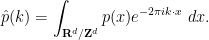
Having discussed uniqueness, we now turn to existence. We begin with the periodic setting in which are required to be -periodic and smooth, so that they can also be viewed (by slight abuse of notation) as functions on the torus . The system (15) is linear and translation-invariant, which strongly suggests that one solve the system using the Fourier transform (which tends to diagonalise linear translation-invariant equations, because the plane waves that underlie the Fourier transform are the eigenfunctions of translation.) Indeed, we may expand as Fourier series

where the Fourier coefficients , , are given by the formulae

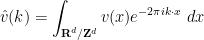
When are smooth, then are rapidly decreasing as , which will allow us to justify manipulations such as interchanging summation and derivatives without difficulty. Expanding out (15) in Fourier series and then comparing Fourier coefficients (which are unique for smooth functions), we obtain the system

for each . As mentioned above, the Fourier transform has diagonalised the system (15), in that there are no interactions between different frequencies , and we now have a decoupled system of vector equations. To solve these equations, we can take the inner product of both sides of (18) with and apply (19) to conclude that

For non-zero , we can then solve for and hence by the formulae

and

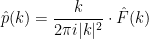
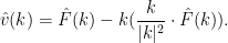
For , these formulae no longer apply; however from (18) we see that , while can be arbitrary (which corresponds to the aforementioned freedom to add an arbitrary constant to ). Thus we have the explicit general solution

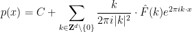
where is an arbitrary constant. Note that if is smooth, then is rapidly decreasing and the functions defined by the above formulae are also smooth.

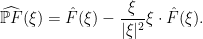
We can write the above general solution in a form similar to (16), (17) as

where, by definition, the inverse Laplacian of a smooth periodic function of mean zero is given by the Fourier series formula

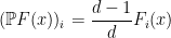
(Note that automatically has mean zero.) It is easy to see that for such functions , thus justifying the choice of notation. We refer to as the (periodic) Leray projection of and denote it , thus in the above solution we have . By construction, is divergence-free, and vanishes whenever is a gradient .

If we require to be -periodic, but do not require to be -periodic, then by the previous uniqueness discussion, the general solution is now

where and are arbitrary.

The above discussion was for smooth periodic functions , but one can make the same construction in other function spaces. For instance, recall that for any , the Sobolev space consists of those elements of whose Sobolev norm

is finite, where we use the “Japanese bracket” convention . (One can also define Sobolev spaces for negative , but we will not need them here.) Basic properties of these Sobolev spaces can be found in this previous post. From comparing Fourier coefficients we see that the operators and defined for smooth periodic functions can be extended without difficulty to (taking values in and respectively), with bounds of the form

Thus, if , then one can solve (15) (in the sense of distributions, at least) with some and , with bounds

In particular, the Leray projection is bounded on . (In fact it is a non-expansive map; see Exercise 16.)

One can argue similarly in the non-periodic setting, as long as one avoids the one-dimensional case which contains some technical divergences. Recall (see e.g., these previous lecture notes on this blog) that functions have a Fourier transform , which for in the dense subclass of is defined by the formula

and then is extended to the rest of by continuous extension in the topology, taking advantage of the Plancherel identity

The Fourier transform is then extended to tempered distributions in the usual fashion (see this previous set of notes).

We then define the Sobolev space for to be the collection of those functions for which the norm

is finite; equivalently, one has

where the Fourier multiplier is defined by

For any vector-valued function in the Schwartz class, we define to be the scalar tempered distribution whose (distributional) Fourier transform is given by the formula

and define the Leray projection to be the vector-valued distribution

or in terms of the (distributional) Fourier transform

Then by using the well-known relationship

between (distributional) derivatives and (distributional) Fourier transforms we see that the tempered distributions

solve the equation (15) in the distributional sense, and hence also in the classical sense since have locally integrable Fourier transforms that are rapidly decreasing away from the origin, and are thus smooth.

As in the periodic case we see that we have the bound

for all Schwartz vector fields (in fact is again a non-expansive map), so we can extend the Leray projection without difficulty to functions. The operator can similarly be extended continuously to a map from to the space of scalar tempered distributions with gradient in , although we will not need to work directly with the pressure much in this course. This allows us to solve (15) in a distributional sense for all .

Remark 15 (Remark removed due to inaccuracy.)

Exercise 16 (Hodge decomposition) Define the following three subspaces of the Hilbert space :

• is the space of all elements of of the form (in the sense of distributions) for some ;
• is the space of all elements of that are weakly harmonic in the sense that (in the sense of distributions).
• is the space of all elements of which take the form

  

  (with the usual summation conventions) for some tensor obeying the antisymmetry property .

• (a) Show that these three spaces are closed subspaces of , and one has the orthogonal decomposition

  

  This is a simple case of a more general splitting known as the Hodge decomposition, which is available for more general differential forms on manifolds.
• (b) Show that on , the Leray projection is the orthogonal projection to .
• (c) Show that the Leray projection is a non-expansive map on for all (that is to say, its operator norm is at most ).

Exercise 17 (Helmholtz decomposition) Define the following two subspaces of the Hilbert space :

• is the space of functions which are divergence-free, by which we mean that in the sense of distributions.
• is the space of functions which are curl-free, by which we mean that in the sense of distributions, where is the rank two tensor with components .

• (a) Show that these two spaces are closed subspaces of , and one has the orthogonal decomposition

  

  This is known as the Helmholtz decomposition (particularly in the three-dimensional case , in which one can interpret as the curl of ).
• (b) Show that on , the Leray projection is the orthogonal projection to .
• (c) Show that the Leray projection is a non-expansive map on for all .

Exercise 18 (Singular integral form of Leray projection) Let . Then the function is locally integrable and thus well-defined as a distribution.

• (a) For , show that the distribution , defined on test functions by the formula

  

  can be expressed in principal value form as

  

  

  where denotes the surface area of the unit sphere in and is the Kronecker delta.
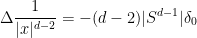
• (b) Conclude in particular the Newtonian potential identity

  

  where (at the risk of a mild notational clash) is the Dirac delta distribution at .
• (c) For a test vector field , establish the explicit form

  

  

• (d) Extend part (c) to the case . (Hint: Replace the role of with , in the spirit of the replica trick from physics.)

Remark 19 One can also solve (15) in -based Sobolev spaces for exponents other than by using Calderón-Zygmund theory and the singular integral form of the Leray projection given in Exercise 18. However, we will try to avoid having to rely on this theory in these notes.

— 3. The heat equation —

We now turn to the study of the heat equation

on a spacetime region , with initial data , where is a fixed constant; we also consider the inhomogeneous analog

with some forcing term .

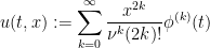
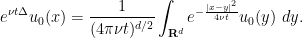
Formally, the solution to the initial value problem for (23) should be given by , and (by the Duhamel formula (6)) the solution to (24) should similarly be

but there are subtleties arising from the unbounded nature of .

The first issue is that even if vanishes and is required to be smooth without any decay hypothesis at infinity, one can have non-uniqueness. The following counterexample is basically due to Tychonoff:

Exercise 20 (Tychonoff example) Let be a real number, and let .

• (a) Show that there exists smooth, compactly supported function , not identically zero, obeying the derivative bounds

  

  for all and . (Hint: one can construct as the convolution of an infinite number of approximate identities , where each is supported on an interval of length , and use the identity repeatedly. To justify things rigorously, one may need to first work with finite convolutions and take limits.)
• (b) With as in part (i) show that the function

  

  is well-defined as a smooth function on that is compactly supported in time, and obeys the heat equation (23) for without being identically zero.
• (c) Show that the initial value problem to (23) is not unique (for any dimension ) if is only required to be smooth, even if vanishes.

Exercise 21 (Kowalevski example)

• (a) Let be the function . Show that there does not exist any solution to (23) that is jointly real analytic in at (that is to say, it can be expressed as an absolutely convergent power series in in a neighbourhood of ).
• (b) Modify the above example by replacing by a function that extends to an entire function on (as opposed to , which has poles at ).

This classic example, due to Sofia Kowalevski, demonstrates the need for some hypotheses on the PDE in order to invoke the Cauchy-Kowaleski theorem.

One can recover uniqueness (forwards in time) by imposing some growth condition at infinity. We give a simple example of this, which illustrates a basic tool in the subject, namely the energy method, which is based on understanding the rate of change of various “energy” integrals of integrands which primarily involve quadratic expressions of the solution or its derivatives. The reason for favouring quadratic expressions is that they are more likely to produce integrals with a definite sign (positive definite or negative definite), such as (squares of) norms or higher Sobolev norms of the solution, particularly after suitable application of integration by parts.

Proposition 22 (Uniqueness with energy bounds) Let , and let be smooth solutions to (24) with common initial data and forcing term such that the norm

of is finite, and similarly for . Then .

Proof: As the heat equation (23) is linear, we may subtract from and assume without loss of generality that , , and . By working with each component separately we may take .

Let be a non-negative test function supported on that equals on . Let be a parameter, and consider the “energy” (or more precisely, “local mass”)

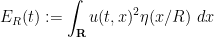for . As , we have . As is smooth and is compactly supported, depends smoothly on , and we can differentiate under the integral sign to obtain

Using (23) we thus have

using the usual summation conventions.

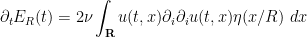
A basic rule of thumb in the energy method is this: whenever one is faced with an integral in which one term in the integrand has much lower regularity (or much less control on regularity) than any other, due to a large number of derivatives placed on that term, one should integrate by parts to move one or more derivatives off of that term to other terms in order to make the distribution of derivatives more balanced (which, as we shall see, tends to make the integrals easier to estimate, or to ascribe a definite sign to). Accordingly, we integrate by parts to write

The first term is non-positive, thus we may discard it to obtain the inequality

Another rule of thumb in the energy method is to keep an eye out for opportunities to express some expression appearing in the integrand as a total derivative In this case, we can write

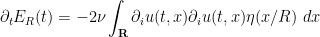
and then integrate by parts to move the derivative on to the much more slowly varying function to conclude

In particular we have a bound of the form

where the subscript indicates that the implied constant can depend on and . Since , we conclude from the fundamental theorem of calculus that

for all (note how it is important here that we evolve forwards in time, rather than backwards). Sending and using the dominated convergence theorem, we conclude that

and thus vanishes identically, as required.

Now we turn to existence for the heat equation, restricting attention to forward in time solutions. Formally, if one solves the heat equation (23), then on taking spatial Fourier transforms

the equation transforms to the ODE

which when combined with the initial condition gives

and hence by the Fourier inversion formula we arrive (formally, at least) at the representation

As we are assuming forward time evolution , the exponential factor here is bounded. In the case that is a Schwartz function, then is also Schwartz, and this formula is certainly well-defined to be smooth in both time and space (and rapidly decreasing in space for any fixed time), and in particular in ; one can easily justify differentiation under the integral sign to conclude that (23) is indeed verified, and the Fourier inversion formula shows that we have the initial data condition . So this is the unique solution to the initial value problem (23) for the heat equation that lies in . By definition we declare the right-hand side of (25) to be , thus

for all and all Schwartz functions ; equivalently, one has

(One can justify this choice of notation using the functional calculus of the self-adjoint operator , as discussed for instance in this previous blog post, but we will not do so here since the Fourier transform is available as a substitute.) It is also clear from (27) that commutes with other Fourier multipliers such as or constant-coefficient differential operators, on Schwartz functions at least.

From (27) and Plancherel’s theorem we see that for is a non-expansive map in (the Schwartz functions of) , and more generally in for any , thus

for any Schwartz and any . Thus by density one can extend the heat propagator for to all of , in a fashion that is a non-expansive map on and more generally on . By a limiting argument, (27) holds almost everywhere for all .

There is also a smoothing effect:

Exercise 23 (Smoothing effect) Let . Show that

for all and .

Exercise 24 (Fundamental solution for the heat equation) For and , establish the identity

for almost every . (Hint: first work with Schwartz functions. Either compute the Fourier transform explicitly, or verify directly that the heat equation initial value problem is solved by the right-hand side.) Conclude in particular that (after modification on a measure zero set if necessary) is smooth for any .

Exercise 25 (Ill-posedness of the backwards heat equation) Show that there exists a Schwartz function with the property that there is no solution to (23) with final data for any . (Hint: choose so that the Fourier transform decays somewhat, but not extremely rapidly. Then argue by contradiction using (27).

Exercise 26 (Continuity in the strong operator topology) For any , let denote the Banach space of functions such that for each , lies in and varies continuously and boundedly in in the strong topology, with norm

Show that if and solves the heat equation on , then with

Similar considerations apply to the inhomogeneous heat equation (24). If and are Schwartz for some , then the function defined by the Duhamel formula

can easily be verified to also be Schwartz and solve (24) with initial data ; by Proposition 22, this is the only such solution in . It also obeys good estimates:

Exercise 27 (Energy estimates) Let , , and be Schwartz functions for some , and let be the solution to the equation

with initial condition given by the Duhamel formula. For any , establish the energy estimate

in two different ways:

• (i) By using the Fourier representation (27) and Plancherel’s formula;
• (ii) By using energy methods as in the proof of Proposition 22. (Hint: first reduce to the case . You may find the arithmetic mean-geometric mean inequality to useful.)

Here of course we are using the norms

and

The energy estimate contains some smoothing effects similar (though not identical) to those in Exercise 23, since it shows that can in principle be one degree of regularity smoother than (if one averages in time in an sense, and the viscosity is not sent to zero), and two degrees of regularity smoother than the forcing term (with the same caveats). As we shall shortly see, this smoothing effect will allow us to handle the nonlinear terms in the Navier-Stokes equations for the purposes of setting up a local well-posedness theory.

Exercise 28 (Distributional solution) Let , let , and let for some . Let be given by the Duhamel formula (28). Show that (24) is true in the spacetime distributional sense, or more precisely that

in the sense of spacetime distributions for any test function supported in the interior of .

Pretty much all of the above discussion can be extended to the periodic setting:

Exercise 29 Let and .

• (a) If is smooth, define by the formula

  

  where are the Fourier coefficients of . Show that extends continuously to a non-expansive map on for every , and that if then the function lies in .
• (b) For and , establish the formula

  

  for almost every , where (by abuse of notation) we identify functions with -periodic functions in the usual fashion.
• (c) If , and and are smooth, show that the function defined by (28) is smooth and solves the inhomogeneous equation (24) with initial data , and that this is the unique smooth solution to that initial value problem.
• (d) If , , and and , are smooth, and is the unique smooth solution to the heat equation with , establish the energy estimate

  

  

  

• (e) If , and , show that the function given by (28) is in and obeys (24) in the sense of spacetime distributions (30).

Remark 30 The heat equation for negative viscosities can be transformed into a positive viscosity heat equation by time reversal: if solves the equation , then solves the equation . Thus one can solve negative viscosity heat equations (also known as backwards heat equations) backwards in time, but one tends not to have well-posedness forwards in time. In a similar spirit, if is positive, one can normalise it to (say) by an appropriate rescaling of the time variable, . However, we will generally keep the parameter non-normalised in preparation for understanding the limit as .

— 4. Local well-posedness for Navier-Stokes —

We now have all the ingredients necessary to create a local well-posedness theory for the Navier-Stokes equations (1).

We first dispose of the one-dimensional case , which is rather degenerate as incompressible one-dimensional fluids are somewhat boring. Namely, suppose that one had a smooth solution to the one-dimensional Navier-Stokes equations

The second equation implies that is just a function of time, , and the first equation becomes

To solve this equation, one can set to be an arbitrary smooth function of time, and then set

for an arbitrary smooth function . If one requires the pressure to be bounded, then vanishes identically, and then is constant in time, which among other things shows that the initial value problem is (rather trivially) well-posed in the category of smooth solutions, up to the ability to alter the pressure by an arbitrary constant . On the other hand, if one does not require the pressure to stay bounded, then one has a lot less uniqueness, since the function is essentially unconstrained.

Now we work in two or higher dimensions , and consider solutions to (1) on the spacetime region . To begin with, we assume that is smooth and periodic in space: for ; we assume is smooth but do not place any periodicity hypotheses on it. Then, by (1), is periodic. In particular, for any and , the function has vanishing gradient and is thus constant in , so that

for all and some function of . The map is a homomorphism for fixed , so we can write for some , which will be smooth since is smooth. We thus have for some smooth -periodic function . By subtracting off the mean, we can further decompose

for some smooth function and some smooth -periodic function which has mean zero at every time.

Note that one can simply omit the constant term from the pressure without affecting the system (1). One can also eliminate the linear term by the following “generalised Galilean transformation“. If are as above, and one lets

be the primitive of , and

be the primitive of , then a short calculation reveals that the smooth function defined by

and the smooth function defined by

solves the Navier-Stokes equations

with having the same initial data as ; conversely, if is a solution to Navier-Stokes, then so is . In particular this reveals a lack of uniqueness for the periodic Navier-Stokes equations that is essentially the same lack of uniqueness that is present for the Leray system: one can add an arbitrary spatially affine function to the pressure by applying a suitable Galilean transform to . On the other hand, we can eliminate this lack of uniqueness by requiring that the pressure be normalised in the sense that and , that is to say we require to be -periodic and mean zero. The above discussion shows that any smooth solution to Navier-Stokes with periodic can be transformed by a Galilean transformation to one in which the pressure is normalised.

Once the pressure is normalised, it turns out that one can recover uniqueness (much as was the case with the Leray system):

Theorem 31 (Uniqueness with normalised pressure) Let be two smooth periodic solutions to (1) on with normalised pressure such that . Then .

Proof: We use the energy method. Write , then subtracting (1) for from we see that is smooth with

and

Now we consider the energy . This varies smoothly with , and we can differentiate under the integral sign to obtain

where

and we have omitted the explicit dependence on and for brevity.

For , we observe the total derivative and integrate by parts to conclude that

since is divergence-free. Similarly, integration by parts shows that vanishes since is divergence-free. Another integration by parts gives

and hence . Finally, from Hölder’s inequality we have

and hence

Since , we conclude from Gronwall’s inequality that for all , and hence is identically zero, thus . Substituting this into (1) we conclude that ; as have mean zero, we conclude (e.g., from Fourier inversion) that , and the claim follows.

Now we turn to existence in the periodic setting, assuming normalised pressure. For various technical reasons, it is convenient to reduce to the case when the velocity field has zero mean. Observe that the right-hand sides , of (1) have zero mean on , thanks to integration by parts. A further integration by parts, using the divergence-free condition , reveals that the transport term also has zero mean:

Thus, we see that the mean is a conserved integral of motion: if is the mean initial velocity, and is a solution to (1) (obeying some minimal regularity hypothesis), then continues to have mean velocity for all subsequent times. On the other hand, if is a smooth periodic solution to (1) with normalised pressure and initial velocity , then the Galilean transform defined by

can be easily verified to be a smooth periodic solution to (1) with normalised pressure and initial velocity . Of course, one can reconstruct from by the inverse tranformation

Thus, up to this simple transformation, solving the initial value problem for (1) for is equivalent to that of , so we may assume without loss of generality that the initial velocity (and hence the velocity at all subsequent times) has zero mean.

A general rule of thumb is that whenever an integral of a solution to a PDE can be proven to vanish (or be equal to boundary terms) by integration by parts, it is because the integrand can be rewritten in “divergence form” – as the divergence of a tensor of one higher rank. (This is because the integration by parts identity arises from the divergence form of the expression .) Thus we expect the transport term to be in divergence form. Indeed, in components we have

since we have the divergence-free condition , we thus have from the Leibniz rule that

We write this in coordinate-free notation as

where is the tensor product and denotes the divergence

Thus we can rewrite (1) as the system

Next, we observe that we can use the Leray projection operator to eliminate the role of the (normalised) pressure. Namely, if are a smooth periodic solution to (1) with normalised pressure, then on applying (which preserves divergence-free vector fields such as and , but annihilates gradients such as ) we conclude an equation that does not involve the pressure at all:

Conversely, suppose that one has a smooth periodic solution to (33) with initial condition for some smooth periodic divergence-free vector field . Taking divergences of both sides of (33), we then conclude that

that is to say obeys the heat equation (23). Since is periodic, smooth, and vanishes at , we see from Exercise 29(c) that vanishes on all of , thus is divergence free on the entire time interval . From (33) and (22) we thus see that if one defines to be the function

(which can easily be verified to be a smooth function in both space and time) then is a smooth periodic solution to (1) with normalised pressure and initial condition (and is thus the unique solution to this system, thanks to Theorem 31). Thus, the problem of finding a smooth solution to (1) in the smooth periodic setting with normalised pressure and divergence-free initial data is equivalent to that of solving (33) with the same initial data.

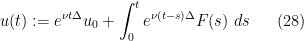
By Duhamel’s formula (Exercise 29(c)), any smooth solution to the initial value problem (33) with obeys the Duhamel formula

(The operator is sometimes referred to as the Oseen operator in the literature.) Conversely, a smooth solution to (34) will solve the initial value problem (33) with initial data .

To obtain existence of smooth periodic solutions (with normalised pressure) to the Navier-Stokes equations with given smooth divergence-free periodic initial data , it thus suffices to find a smooth periodic solution to the integral equation (34). We will achieve this by a two-step procedure:

• (i) (Existence at finite regularity) Construct a solution to (34) in a certain function space with a finite amount of regularity (assuming that the initial data has a similarly finite amount of regularity); and then
• (ii) (Propagation of regularity) show that if is in fact smooth, then the solution constructed in (i) is also smooth.

The reason for this two step procedure is that one wishes to solve (34) using iteration-type methods (which for instance power the contraction mapping theorem that was used to prove the Picard existence theorem); however the function space that one ultimately wishes the solution to lie in is not well adapted for such iteration (for instance, it is not a Banach space, instead being merely a Fréchet space). Instead, we iterate in an auxiliary lower regularity space first, and then “bootstrap” the lower regularity to the desired higher regularity. Observe that the same situation occured with the Picard existence theorem, where one performed the iteration in the low regularity space , even though ultimately one desired the solution to be continuously differentiable or even smooth.

Of course, to run this procedure, one actually has to write down an explicit function space in which one will perform the iteration argument. Selection of this space is actually a non-trivial matter and often requires a substantial amount of trial and error, as well as experience with similar iteration arguments for other PDE. Often one is guided by the function space theory for the linearised counterpart of the PDE, which in this case is the heat equation (23). As such, the following definition can be at least partially motivated by the energy estimates in Exercise 29(d).

Definition 32 (Mild solution) Let , , and let be divergence-free, where denotes the subspace of consisting of mean zero functions. An -mild solution (or Fujita-Kato mild solution to the Navier-Stokes equations with initial data is a function in the function space

that obeys the integral equation (34) (in the sense of distributions) for all . We say that is a mild solution on if it is a mild solution on for every .

Remark 33 The definition of a mild solution could be extended to those choices of initial data that are not divergence-free, but then this solution concept no longer has any direct connection with the Navier-Stokes equations, so we will not consider such “solutions” here. Similarly, one could also consider mild solutions without the mean zero hypothesis, but the function space estimates are slightly less favourable in this setting and so we shall restrict attention to mean zero solutions only.

Note that the regularity on places in (with plenty of room to spare), which is more than enough regularity to make sense of the right-hand side of (34) in a (spacetime) distributional sense at least. One can also define mild solutions for other function spaces than the one provided here, but we focus on this notion for now, which was introduced in the work of Fujita and Kato. We record a simple compatibility property of mild solutions:

Exercise 34 (Splitting) Let , , let be divergence-free, and let

Let . Show that the following are equivalent:

• (i) is an mild solution to the Navier-Stokes equations on with initial data .
• (ii) is an mild solution to the Navier-Stokes equations on with initial data , and the translated function defined by is an mild solution to the Navier-Stokes equations with initial condition .

To use this notion of a mild solution, we will need the following harmonic analysis estimate:

Proposition 35 (Product estimate) Let , and let . Then one has , with the estimate

When this claim follows immediately from Hölder’s inequality. For the claim is similarly immediate from the Leibniz rule and the triangle and Hölder inequalities (noting that is comparable to . For more general the claim is not quite so immediate (for instance, when one runs into difficulties controlling the intermediate term arising in the Leibniz expansion of ). Nevertheless the bound is still true. However, to prove it we will need to introduce a tool from harmonic analysis, namely Littlewood-Paley theory, and we defer the proof to the appendix.

We also need a simple case of Sobolev embedding:

Exercise 36 (Sobolev embedding)

• (a) If , show that for any , one has with

  

• (b) Show that the inequality fails at .
• (c) Establish the same statements with replaced by throughout.

In particular, combining this exercise with Proposition 35 we see that for , is a Banach algebra:

Now we can construct mild solutions at high regularities .

Theorem 37 (Local well-posedness of mild solutions at high regularity) Let , and let be divergence-free. Then there exists a time

and an mild solution to (34). Furthermore, this mild solution is unique.

The hypothesis is not optimal; we return to this point later in these notes.

Proof: We begin with existence. We can write (34) in the fixed point form

where

We remark that this expression automatically has mean zero since has mean zero. Let denote the function space

with norm

This is a Banach space. Because of the mean zero restriction on , we may estimate

Note that if , then by (35), which by Exercise 29(d) (and the fact that commutes with and is a non-expansive map on ) implies that . Thus is a map from to . In fact we can obtain more quantitative control on this map. By using Exercise 29(d), (35), and the Hölder bound

we have

Thus, if we set for a suitably large constant , and set for a sufficienly small constant , then maps the closed ball in to itself. Furthermore, for , we have by similar arguments to above

and hence if the constant is chosen small enough, is also a contraction (with constant, say, ) on . Thus there exists such that , thus is an mild solution.

Now we show that it is the only mild solution. Suppose for contradiction that there is another mild solution with the same initial data . This solution might not lie in , but it will lie in for some . By the same arguments as above, if is sufficiently small depending on then will be a contraction on , which implies that and agree on . Now we apply Exercise 34 to advance in time by and iterate this process (noting that depends on but does not otherwise depend on or ) until one concludes that on all of .

Iterating this as in the proof of Theorem 8, we have

Theorem 38 (Maximal Cauchy development) Let , and let be divergence-free. Then there exists a time and an mild solution to (34), such that if then as . Furthermore, and are unique.

In principle, if the initial data belongs to multiple Sobolev spaces the maximal time of existence could depend on (so that the solution exits different regularity classes at different times). However, this is not the case, because there is an -independent blowup criterion:

Proposition 39 (Blowup criterion) Let be as in Theorem 38. If , then .

Note from Exercise 36 that is finite for any . This shows that is the unique time at which the norm “blows up” (becomes infinite) and thus is independent of .

Proof: Suppose for contradiction that but that the quantity was finite. Let be parameters to be optimised in later. We define the norm

As is a mild solution, this expression is finite.

We adapt the proof of Theorem 37. Using Exercise 29(d) (and Exercise 34) we have

Again we discard and use (a variant of) (37) to conclude

If we now use Proposition 35 in place of (35), we conclude that

If we choose to be sufficiently close to (depending on and ), we can absorb the second term on the RHS into the LHS and conclude that

In particular, stays bounded as , contradicting Theorem 38.

Corollary 40 (Existence of smooth solutions) If is smooth and divergence free then there is a and a smooth periodic solution to the Navier-Stokes equations on with normalised pressure such that if , then . Furthermore, and are unique.

Proof: As discussed previously, we may assume without loss of generality that has mean zero. As is periodic and smooth, it lies in for every . From the preceding discussion we already have and a function that is an mild solution for every , and with if is finite. It will suffice to show that is smooth, since we know from preceding discussion that a smooth solution to (33) can be converted to a smooth solution to (1).

By Exercise 29, one has

in the sense of spacetime distributions. The right-hand side lies in for every , hence the left-hand side does also; this makes lie in . It is then easy to see that this implies that the right-hand side of the above equation lies in for every , and so now lies in for every . Iterating this (and using Sobolev embedding) we conclude that is smooth in space and time, giving the claim.

Remark 41 When , it is a notorious open problem whether the maximal lifespan given by the above corollary is always infinite.

Exercise 42 (Instantaneous smoothing) Let , let be divergence-free, and let be the maximal Cauchy development provided by Theorem 38. Show that is smooth on (note the omission of the initial time ). (Hint: first show that is a mild solution for arbitrarily small .)

Exercise 43 (Lipschitz continuous dependence on initial data) Let , let , and let be divergence-free. Suppose one has an mild solution to the Navier-Stokes equations with initial data . Show that there in a neighbourhood of in (the divergence-free elements of) in , such that for every , there exists an mild solution to the Navier-Stokes equations with initial data with the map from to Lipschitz continuous (using the metric for the initial data and the metric for the solution ).

Now we discuss the issue of relaxing the regularity condition in the above theory. The main inefficiency in the above arguments is the use of the crude estimate (37), which sacrifices some of the exponent in time in exchange for extracting a positive power of the lifespan that can be used to create a contraction mapping, as long as is small enough. It turns out that by using a different energy estimate than Exercise 29(d), one can avoid such an exchange, allowing one to construct solutions at lower regularity, and in particular at the “critical” regularity of . Furthermore, in the category of smooth solutions, one can even achieve the desirable goal of ensuring that the time of existence is infinite – but only provided that the initial data is small. More precisely,

Proposition 44 Let and let . Then the function defined by the Duhamel formula

also has mean zero for all , and obeys the estimates

Proof: By Minkowski’s integral inequality, it will suffice to establish the bounds in the case . The first two norms of the left-hand side are already established by Exercise 29(d), so it remains to establish the estimate

By working with the rescaled function (and also rescaling ), we may normalise . By a limiting argument we may assume without loss of generality that is Schwarz. We cannot directly apply Exercise 36 here due to the failure of endpoint Sobolev embedding; nevertheless we may argue as follows. For any , we see from (31), the mean zero hypothesis, and the triangle inequality that

To proceed further, we choose an exponent such that

(for instance one can take ), and use Cauchy-Schwarz to bound

As , one has the bound

(which can be verified using the integral test for , while for it is easy to bound the LHS by ) and hence

Taking norms and using Fubini’s theorem, we conclude

As , the inner integral can be estimated as

and the claim follows.

This gives the following small data global existence result, also due to Fujita and Kato:

Theorem 45 (Small data global existence) Suppose that is divergence-free with norm at most , where is a sufficiently small constant depending only on . Then there exists a mild solution to the Navier-Stokes equations on . Furthermore, if is smooth, then this mild solution is also smooth.

Proof: By working with the rescaled function , we may normalise . Let denote the Banach space of functions

with the obvious norm

Let be the Duhamel operator (36). If , then by Proposition 44 and Lemma 35 one has

In particular, maps to . A similar argument establishes the bound

for all . For small enough, will be a contraction on for some absolute constant depending only on , and hence has a fixed point which will be the desired mild solution.

Now suppose that is smooth. Let , and let be the maximal Cauchy development provided by Theorem 38. For any , if one defines

then the preceding arguments give

thus either or . On the other hand, depends continuously on and converges to as . For small enough, this implies that for all (this is an example of a “continuity argument”). Next, if we set

then repeating the previous arguments also gives

as is finite and , we conclude (for small enough) that

In particular we have

for all , and hence by Theorem 38 we have . The argument used to prove Corollary 40 shows that is smooth. From the bounds on we see that, lies in with norm at most , and so agrees with the fixed point of located previously. The claim follows.

Remark 46 Modifications of this argument also allow one to establish local existence of mild solutions when the initial data lies in , but has large norm rather than norm less than ; see Exercise 47 below. However, in this case one does not have a lower bound on the time of existence that depends only on the norm of the data, as was the case with Theorem 37. Further modification of the argument also allows one to extend Theorem 38 to the entire “subcritical” range of regularities . See the paper of Fujita and Kato for details.

Exercise 47 (Large data critical local existence) Suppose that is divergence-free. Show that there exists and a mild solution to the Navier-Stokes equations on . Furthermore, if is smooth, then this mild solution is also smooth. (Hint: By choosing small enough, one can ensure that the linear evolution is small in and norms. Now run a contraction mapping argument in a space of functions that are small in and norm and bounded in norm. One will have to carefully choose all the relevant parameters in the right order, and to choose an appropriate weighted metric on this space of functions, in order to actually obtain a contraction.

We now turn attention to the non-periodic case in two and higher dimensions . The theory is largely identical, though with some minor technical differences. Unlike the periodic case, we will not attempt to reduce to the case of having mean zero (indeed, we will not even assume that is absolutely integrable, so that the mean might not even be well defined).

In the periodic case, we focused initially on smooth solutions. Smoothness is not sufficient by itself in the non-periodic setting to provide a good well-posedness theory, as we already saw in Section 3 when discussing the linear heat equation; some additional decay at spatial infinity is needed. There is some flexibility as to how much smoothness to prescribe. Let us say that a solution to Navier-Stokes is classical if and are smooth, and furthermore lies in for every .

Now we work on normalising the pressure. Suppose is a classical solution. As before we may write the Navier-Stokes equation in divergence form as (32). Taking a further divergence we obtain the equation

The function belongs to for every , so if we define the normalised pressure

via the Fourier transform as

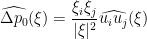then will also belong to for every . We then have for some harmonic function that is smooth in space and continuous in time (thus all spatial derivatives exist and are continuous in both space and time). To control this harmonic function, we return to (32), which we write as

where

and apply the fundamental theorem of calculus to conclude that

The left-hand side is harmonic (thanks to differentiating under the integral sign), and the right-hand side lies in (in fact it is in for every ), hence both sides vanish. By the fundamental theorem of calculus this implies that vanishes identically, thus is constant in space. One can then subtract it from the pressure without affecting (1); also, we now have

which implies that for all , which by the Navier-Stokes equations implies that for all ; iterating this we find eventually that all time derivatives of exist in , and hence is smooth. Thus, in the category of classical solutions, at least, we may assume without loss of generality that we have normalised pressure

in which case the Navier-Stokes equations may be written as before as (33). (See also this paper of mine for some variants of this argument.)

Exercise 48 (Uniqueness with normalised pressure) Let be two smooth classical solutions to (1) on with normalised pressure such that . Then .

We can now define the notion of a Fujita-Kato mild solution as before, except that we replace all mention of the torus with the Euclidean space , and omit all requirements for the solution to be of mean zero. As stated in the appendix, the product estimate in Proposition 35 continues to hold in , so one can obtain the analogue of Theorem 37, Theorem 38, Proposition 39, and Corollary 40 on by repeating the proofs with the obvious changes; we leave the details as an exercise for the interested reader.

Exercise 49 Establish an analogue of Proposition 44 on , using the homogeneous Sobolev space defined to be the closure of the Schwartz functions with respect to the norm

and use this to state and prove an analogue of Theorem 45.

— 5. Heuristics —

There are several further extensions of these types of local and global existence results for smooth solutions, in which the role of the Sobolev spaces here are replaced by other function spaces. For instance, in three dimensions in the non-periodic setting, the role of the critical space was replaced by the larger critical space by Kato, and to the even larger space by Koch and Tataru, who also gave evidence that the latter space essentially the limit of the method; in even larger spaces such as the Besov space , there are constructions of Bourgain and Pavlovic that demonstrate ill-posedness in the sense of “norm inflation” – solutions that start from arbitrarily small norm data but end up being arbitrarily large in arbitrarily small amounts of time. (This grossly abbreviated history skips over dozens of other results, both positive and negative, in yet further function spaces, such as Morrey spaces or Besov spaces. See for instance the recent text of Lemarie-Rieusset for a survey.)

Rather tham detail these other results, let us present instead a scaling heuristic which can be used to interpret these results (and can clarify why all the positive well-posedness results discussed here involve either “subcritical” or “critical” function spaces, rather than “supercritical” ones). For simplicity we restrict our discussion to the non-periodic setting , although the discussion here could also be adapted without much difficulty to the periodic setting (which effectively just imposes an additional constraint on the frequency parameter to be introduced below).

In this heuristic discussion, we assume that any given time , the velocity field is primarily located at a certain frequency (or equivalently, at a certain wavelength ) in the sense that the spatial Fourier transform is largely concentrated in the region . We also assume that at this time, the solution has an amplitude , in the sense that tends to be of order in magnitude in the region where it is concentrated. (We are deliberately leaving terms such as “concentrated” vague for the purposes of this discussion.) Using this ansatz, one can then heuristically compute the magnitude of various terms in the Navier-Stokes equations (1) or the projected version (33). For instance, if has amplitude and frequency , then should have amplitude (and frequency ), since the Laplacian operator multiplies the Fourier transform by ; one can also take a more “physical space” viewpoint and view the second derivatives in as being roughly like dividing out by the wavelength twice. Thus we see that the viscosity term in (1) or (33) should have size about . Similarly, the expression in (33) should have magnitude and frequency (or maybe slightly less due to cancellation), so and hence should have magnitude . The terms and in (1) can similarly be computed to have magnitude . Finally, if the solution oscillates (or blows up) in time in intervals of length (which one can think of as the natural time scale for the solution), then the term should have magnitude .

This leads to the following heuristics:

• If (or equivalently if ), then the viscosity term dominates the nonlinear terms in (1) or (33), and one should expect the Navier-Stokes equations to behave like the heat equation (23) in this regime. In particular solutions should exist and maintain (or even improve) their regularity as long as this regime persists. To balance the equation (1) or (33), one expects , so the natural time scale here is .
• If (or equivalently if ), then nonlinear effects dominate, and the behaviour is likely to be quite different to that of the heat equation. One now expects , so the natural time scale here is . In particular, one could theoretically have blowup or other bad behaviour after this time scale.

As a general rule of thumb, the known well-posedness theory for the Navier-Stokes equation is only applicable when the hypotheses on the initial data (and on the timescale being considered) is compatible either with the viscosity-dominated regime , or the time-limited regime . Outside of these regimes, we expect the evolution to be highly nonlinear in nature, and techniques such as the ones in this set of notes, which are primarily based on approximating the evolution by the linear heat flow, are not expected to apply.

Let’s discuss some of the results in this set of notes using these heuristics. Suppose we are given that the initial data is bounded in norm by some bound :

As in the above heuristics, we assume that exhibits some amplitude and frequency . Heuristically, the norm of should resemble times the norm of , which should be roughly , where is the volume of the region where is concentrated in. Thus we morally have a bound of the form

To use this bound, we invoke (at a heuristic level) the uncertainty principle , which indicates that the data should be spatially spread out at a scale of at least the wavelength , which implies that the volume should be at least . Thus we have

Suppose we have , then we have the crude bound

so we expect to have an amplitude bound . If we are in the nonlinear regime , this implies that , and so the natural time scale here is lower bounded by . This matches up with the local existence time given in Theorem 37 (or the non-periodic analogue of this theorem). However, the use of the crude bound (39) suggests that one can make improvements to this bound when is far from :

Exercise 50 If , make a heuristic argument as to why the optimal lower bound for the time of existence for the Navier-Stokes equation in terms of the norm of the initial data should take the form

In a similar spirit, suppose we have the smallness hypothesis

on the critical norm , then a similar analysis to above leads to

and hence we will be in the viscosity dominated regime if is small enough, regardless of what time scale one uses; this is consistent with the global existence result in Theorem 45. On the other hand, if the norm is much larger than , then can be larger than , and we can fail to be in the viscosity dominated regime at any choice of frequency ; setting to be a large multiple of and sending to infinity, we see that the natural time scale could be arbitrarily small.

Finally, if one only controls a supercritical norm such as for some , this gives a bound on a quantity of the form , which allows one to leave the viscosity dominated regime (with plenty of room to spare) when is large, creating examples of initial data for which the natural time scale can be made arbitrarily small. As increases (restricting to, say, powers of two), the supercritical norm of these examples decays geometrically, so one can superimpose an infinite number of these examples together, leading to a choice of initial data with arbitrarily small supercritical norm for which the natural time scale is in fact zero. This strongly suggests that there is no good local well-posedness theory at such regularities.

Exercise 51 Discuss the product estimate in Proposition 35, the Sobolev estimate in Exercise 36, and the energy estimates in Exercise 29(d) and Proposition 44 using the above heuristics.

Remark 52 These heuristics can also be used to locate errors in many purported solutions to the Navier-Stokes global regularity problem that proceed through a sequence of estimates on a Navier-Stokes solution. At some point, the estimates have to rule out the scenario that the solution leaves the viscosity-dominated regime at larger and larger frequencies (and at smaller and smaller time scales ), with the time scales converging to zero to achieve a finite time blowup. If the estimates in the proposed solution are strong enough to heuristically rule out this scenario by the end of the argument, but not at the beginning of the argument, then there must be some step inside the argument where one moves from “supercritical” estimates that are too weak to rule out this scenario, to “critical” or “subcritical” estimates which are capable of doing so. This step is often where the error in the argument may be found.

The above heuristics are closely tied to the classification of various function space norms as being “subcritical”, “supercritical”, or “critical”. Roughly speaking, a norm is subcritical if bounding that norm heuristically places one in the linear-dominated regime (which, for Navier-Stokes, is the viscosity-dominated regime) at high frequencies; critical if control of the norm very nearly places one in the linear-dominated regime at high frequencies; and supercritical if control of the norm completely fails to place one in the linear-dominated regime at high frequencies. When the equation in question enjoys a scaling symmetry, the distinction between subcritical, supercritical, and critical norms can be made by seeing how the the top-order component of these norms vary with respect to scaling a function to be high frequency. In the case of the Navier-Stokes equations (1), the scaling is given by the formulae

with the initial data similarly being scaled to

Here is a scaling parameter; as , the functions are being sent to increasingly fine scales (i.e., high frequencies). One easily checks that if solves the Navier-Stokes equations (1) with initial data , then solves the same equations with initial data ; similarly for other formulations of the Navier-Stokes equations such as (33) or (34). (In terms of the parameters from the previous heuristic discussion, this scaling corresponds to the map .)

Typically, if one considers a function space norm of (or of or ) in the limit , the top order behaviour will be given by some power of . A norm is called subcritical if the exponent is positive, supercritical if the exponent is negative, and critical if the exponent is zero. For instance, one can calculate the Fourier transform

and hence

As , this expression behaves like to top order; hence the norm is subcritical when , supercritical when , and critical when .

Another way to phrase this classification is to use dimensional analysis. If we use to denote the unit of length, and the unit of time, then the velocity field should have units , and the terms and in (1) then have units . To be dimensionally consistent, the kinematic viscosity must then have the units , and the pressure should have units . (This differs from the usual units given in physics to the pressure, which is where is the unit of mass; the discrepancy comes from the choice to normalise the density, which usually has units , to equal .) If we fix to be a dimensionless constant such as , this forces a relation between the time and length units, so now and have the units and respectively (compare with (40) and (41)). Of course will then also have units . One can then declare a function space norm of , , or to be subcritical if its top order term has units of a negative power of , supercritical if this is a positive power of , and critical if it is dimensionless. For instance, the top order term in is the norm of ; as has the units of , and Lebesgue measure has the units of , we see that has the units of , giving the same division into subcritical, supercritical, and critical spaces as before.

— 6. Appendix: some Littlewood-Paley theory —

We now prove Proposition 35. By a limiting argument it suffices to establish the claim for smooth . The claim is immediate from Hölder’s inequality when , so we will assume . For brevity we shall abbreviate as , and similarly for , etc..

We use the technique of Littlewood-Paley projections. Let be an even bump function (depending only on ) that equals on and is supported on ; for the purposes of asymptotic notation, any bound that depends on can thus be thought of as depending on instead. For any dyadic integer (by which we mean an integer that is a power of ), define the Littlewood-Paley projections on periodic smooth functions by the formulae

and (for )

so one has the Littlewood-Paley decomposition

Here and in the sequel is always understood to be restricted to be a dyadic integer.

The key point of this decomposition is that the and Sobolev norms of the individual components of this decomposition are easier to estimate than the original function . The following estimates in particular will suffice for our applications:

Exercise 53 (Basic Littlewood-Paley estimates)

• (a) For any dyadic integer , show that

  

  where is the inverse Fourier transform of on , and the difference between the coset and the shift is defined in the obvious fashion. In particular if is real-valued then so is and . Conclude the Bernstein inequality

  

  for all smooth functions , all and ; in particular

  

  (Recall our convention that constants that depend on can also be thought of as depending just on .) By the triangle inequality, the same estimates also hold for , .
• (b) For any , show that

  

Remark 54 The more advanced Littlewood-Paley inequality, which is usually proven using the Calderón-Zygmund theory of singular integrals, asserts that

for any . However, we will not use this estimate here.

We return now to the proof of Proposition 35. Let be as above. By Exercise 53, it suffices to establish the bounds

and

The estimate (42) follows by dropping (using Exercise 53) and applying Hölder’s inequality, so we turn to (43). We may restrict attention to those terms where (say) since the other terms can be treated by the same argument used to prove (42).

The basic strategy here is to split the product (or the component of this product) into paraproducts in which some constraint is imposed between the frequencies of the and terms. There are many ways to achieve this splitting; we will use

By the triangle inequality, it suffices to show the estimates

and

We begin with (44). We can expand further

The key point now is that (by inspecting the Fourier series expansions) the first term on the RHS vanishes, and the summands in the second term also vanish unless . Thus

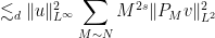and the claim follows by summing in , interchanging the summations, and using Exercise 53. Now we prove (45). We bound

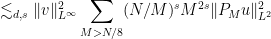using Cauchy-Schwarz, and the claim again follows by summing in , interchanging the summations, and using Exercise 53.

There is an essentially identical theory in the non-periodic setting, in which the role of smooth periodic functions are now replaced by Schwartz functions, the Littlewood-Paley projections are now defined as

and is defined as before.

Exercise 55 (Non-periodic Littlewood-Paley theory) With now denoting instead of , and similarly for other function spaces, establish the non-periodic analogue of Exercise 53 for Schwartz functions .

In particular, one obtains the non-periodic analogue of Proposition 35 by repeating the proof verbatim.