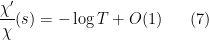
A useful rule of thumb in complex analysis is that holomorphic functions  behave like large degree polynomials
  . This can be evidenced for instance at a “local” level by the Taylor series expansion for a complex analytic function in the disk, or at a “global” level by factorisation theorems such as the Weierstrass factorisation theorem (or the closely related Hadamard factorisation theorem). One can truncate these theorems in a variety of ways (e.g., Taylor’s theorem with remainder) to be able to approximate a holomorphic function by a polynomial on various domains.
In some cases it can be convenient instead to work with polynomials  of another variable
  such as
  (or more generally
  for a scaling parameter
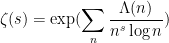
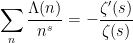
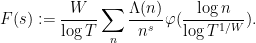
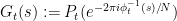
  ). In the case of the Riemann zeta function, defined by meromorphic continuation of the formula

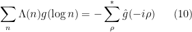
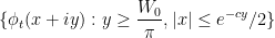
one ends up having the following heuristic approximation in the neighbourhood of a point  on the critical line:
Heuristic 1 (Polynomial approximation) Let  be a height, let
  be a “typical” element of
 ![{[T,2T]}](https://s0.wp.com/latex.php?latex=%7B%5BT%2C2T%5D%7D&bg=ffffff&fg=000000&s=0&c=20201002) , and let
, and let  be an integer. Let
  be the linear change of variables
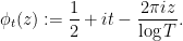
Then one has an approximation

for  and some polynomial
  of degree .
The requirement  is necessary since the right-hand side is periodic with period in the
  variable (or period
  in the
  variable), whereas the zeta function is not expected to have any such periodicity, even approximately.
Let us give two non-rigorous justifications of this heuristic. Firstly, it is standard that inside the critical strip (with  ) we have an approximate form

of (11). If we group the integers  from
from  to
to  into bins depending on what powers of
  they lie between, we thus have

For with and  we heuristically have

and so

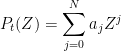
where  are the partial Dirichlet series
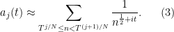
This gives the desired polynomial approximation.
A second non-rigorous justification is as follows. From factorisation theorems such as the Hadamard factorisation theorem we expect to have
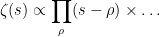
where  runs over the non-trivial zeroes of
  , and there are some additional factors arising from the trivial zeroes and poles of which we will ignore here; we will also completely ignore the issue of how to renormalise the product to make it converge properly. In the region
  , the dominant contribution to this product (besides multiplicative constants) should arise from zeroes that are also in this region. The Riemann-von Mangoldt formula suggests that for “typical” one should have about such zeroes. If one lets
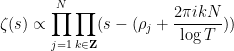
  be any enumeration of zeroes closest to , and then repeats this set of zeroes periodically by period , one then expects to have an approximation of the form
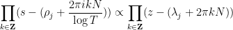
again ignoring all issues of convergence. If one writes and  , then Euler’s famous product formula for sine basically gives
(here we are glossing over some technical issues regarding renormalisation of the infinite products, which can be dealt with by studying the asymptotics as  ) and hence we expect

This again gives the desired polynomial approximation.
Below the fold we give a rigorous version of the second argument suitable for “microscale” analysis. More precisely, we will show
Theorem 2 Let  be an integer going sufficiently slowly to infinity. Let
  go to zero sufficiently slowly depending on . Let be drawn uniformly at random from . Then with probability
  (in the limit
  ), and possibly after adjusting by , there exists a polynomial
  of degree and obeying the functional equation (9) below, such that

whenever  .
.
It should be possible to refine the arguments to extend this theorem to the mesoscale setting by letting be anything growing like  , and
, and  anything growing like
  ; also we should be able to delete the need to adjust by . We have not attempted these optimisations here.
Many conjectures and arguments involving the Riemann zeta function can be heuristically translated into arguments involving the polynomials , which one can view as random degree polynomials if is interpreted as a random variable drawn uniformly at random from . These can be viewed as providing a “toy model” for the theory of the Riemann zeta function, in which the complex analysis is simplified to the study of the zeroes and coefficients of this random polynomial (for instance, the role of the gamma function is now played by a monomial in ). This model also makes the zeta function theory more closely resemble the function field analogues of this theory (in which the analogue of the zeta function is also a polynomial (or a rational function) in some variable , as per the Weil conjectures). The parameter is at our disposal to choose, and reflects the scale  at which one wishes to study the zeta function. For “macroscopic” questions, at which one wishes to understand the zeta function at unit scales, it is natural to take
  (or very slightly larger), while for “microscopic” questions one would take close to and only growing very slowly with . For the intermediate “mesoscopic” scales one would take somewhere between and
  . Unfortunately, the statistical properties of
  are only understood well at a conjectural level at present; even if one assumes the Riemann hypothesis, our understanding of is largely restricted to the computation of low moments (e.g., the second or fourth moments) of various linear statistics of and related functions (e.g.,
  ,
,  , or
, or  ).
).
Let’s now heuristically explore the polynomial analogues of this theory in a bit more detail. The Riemann hypothesis basically corresponds to the assertion that all the zeroes of the polynomial lie on the unit circle  (which, after the change of variables
  , corresponds to being real); in a similar vein, the GUE hypothesis corresponds to having the asymptotic law of a random scalar
  times the characteristic polynomial of a random unitary
  matrix. Next, we consider what happens to the functional equation

where

A routine calculation involving Stirling’s formula reveals that

with  ; one also has the closely related approximation
and hence

when  . Since
  , applying (5) with and using the approximation (2) suggests a functional equation for :

or in terms of  ,
,

where  is the polynomial with all the coefficients replaced by their complex conjugate. Thus if we write
then the functional equation can be written as

We remark that if we use the heuristic (3) (interpreting the cutoffs in the summation in a suitably vague fashion) then this equation can be viewed as an instance of the Poisson summation formula.
Another consequence of the functional equation is that the zeroes of are symmetric with respect to inversion  across the unit circle. This is of course consistent with the Riemann hypothesis, but does not obviously imply it. The phase
  is of little consequence in this functional equation; one could easily conceal it by working with the phase rotation
  of instead.
One consequence of the functional equation is that 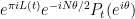 is real for any
  ; the same is then true for the derivative
  . Among other things, this implies that
  cannot vanish unless
  does also; thus the zeroes of
  will not lie on the unit circle except where has repeated zeroes. The analogous statement is true for ; the zeroes of
  will not lie on the critical line except where has repeated zeroes.
Relating to this fact, it is a classical result of Speiser that the Riemann hypothesis is true if and only if all the zeroes of the derivative of the zeta function in the critical strip lie on or to the right of the critical line. The analogous result for polynomials is
Proposition 3 We have

(where all zeroes are counted with multiplicity.) In particular, the zeroes of all lie on the unit circle if and only if the zeroes of  lie in the closed unit disk.
Proof: From the functional equation we have

Thus it will suffice to show that and have the same number of zeroes outside the closed unit disk.
Set  , then
  is a rational function that does not have a zero or pole at infinity. For
  not a zero of , we have already seen that and are real, so on dividing we see that
  is always real, that is to say
(This can also be seen by writing  , where
  runs over the zeroes of , and using the fact that these zeroes are symmetric with respect to reflection across the unit circle.) When is a zero of , has a simple pole at with residue a positive multiple of , and so stays on the right half-plane if one traverses a semicircular arc around outside the unit disk. From this and continuity we see that stays on the right-half plane in a circle slightly larger than the unit circle, and hence by the argument principle it has the same number of zeroes and poles outside of this circle, giving the claim.
From the functional equation and the chain rule, is a zero of if and only if  is a zero of
  . We can thus write the above proposition in the equivalent form

One can use this identity to get a lower bound on the number of zeroes of by the method of mollifiers. Namely, for any other polynomial  , we clearly have


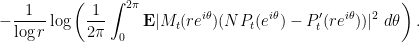
By Jensen’s formula, we have for any  that
that


We therefore have

As the logarithm function is concave, we can apply Jensen’s inequality to conclude

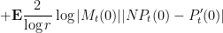
where the expectation is over the parameter. It turns out that by choosing the mollifier carefully in order to make  behave like the function (while keeping the degree small enough that one can compute the second moment here), and then optimising in
  , one can use this inequality to get a positive fraction of zeroes of on the unit circle on average. This is the polynomial analogue of a classical argument of Levinson, who used this to show that at least one third of the zeroes of the Riemann zeta function are on the critical line; all later improvements on this fraction have been based on some version of Levinson’s method, mainly focusing on more advanced choices for the mollifier and of the differential operator
  that implicitly appears in the above approach. (The most recent lower bound I know of is
  , due to Pratt and Robles. In principle (as observed by Farmer) this bound can get arbitrarily close to if one is allowed to use arbitrarily long mollifiers, but establishing this seems of comparable difficulty to unsolved problems such as the pair correlation conjecture; see this paper of Radziwill for more discussion.) A variant of these techniques can also establish “zero density estimates” of the following form: for any
  , the number of zeroes of that lie further than
  from the unit circle is of order
  on average for some absolute constant
  . Thus, roughly speaking, most zeroes of lie within
  of the unit circle. (Analogues of these results for the Riemann zeta function were worked out by Selberg, by Jutila, and by Conrey, with increasingly strong values of
  .)
.)
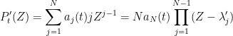
The zeroes of tend to live somewhat closer to the origin than the zeroes of . Suppose for instance that we write

where  are the zeroes of , then by evaluating at zero we see that

and the right-hand side is of unit magnitude by the functional equation. However, if we differentiate
where  are the zeroes of , then by evaluating at zero we now see that

The right-hand side would now be typically expected to be of size  , and so on average we expect the
  to have magnitude like
  , that is to say pushed inwards from the unit circle by a distance roughly
  . The analogous result for the Riemann zeta function is that the zeroes of
  at height
  lie at a distance roughly
  to the right of the critical line on the average; see this paper of Levinson and Montgomery for a precise statement.
— 1. An exact factorisation of —
In this section we give an an exact factorisation of into a “mesoscopic” part involving a finite Dirichlet series relating to the von Mangoldt function, and a “microscopic” part involving nearby zeroes; this can be viewed as an interpolant between the classical formula
for  on one hand, and the Weierstrass or Hadamard factorisations on the other. This factorisation will be useful in the eventual proof of Theorem 2. (UPDATE: I have since learned that this factorisation was previously introduced by Gonek, Hughes, and Keating (see also this later paper of Gonek), for essentially the same purposes as in this post.)
The starting point will be the explicit formula, which we use in the form
for any test function  supported in
  , where
  is the von Mangoldt function,
  is the Fourier transform

and  sums over all zeroes of the Riemann zeta function (both trivial and non-trivial), together with the pole at
  counted wiht multiplicity
  . See for instance Exercise 46 of this previous blog post. If
  is a test function that equals near the origin, and
  has sufficiently large real part, then this formula, together with a limiting argument, implies that

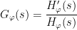
where
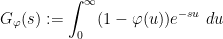
is the Laplace transform of  . Since
we conclude that
when the real part of  is sufficiently large. We can integrate by parts to write

and now it is clear  extends meromorphically to the entire complex plane with a simple pole at
  with residue
  ; also, since
  is smooth and supported in some compact subinterval
 ![{[c_1,c_2]}](https://s0.wp.com/latex.php?latex=%7B%5Bc_1%2Cc_2%5D%7D&bg=ffffff&fg=000000&s=0&c=20201002) of
of  , we see that we have estimates of the form

for any  , thus
  decays exponentially as
  and is rapidly decreasing as
  . (If
. (If  is not merely smooth, but is in fact in a Gevrey class, one can improve the
  factor to
  for some and
  . This is basically the maximum decay one can hope for here thanks to the Paley-Wiener theorem (or the more advanced Beurling-Malliavin theorem). However, we will not need such strong decay here.) Both sides of (11) now extend meromorphically to the entire complex plane and so the identity (11) holds for all other than the zeroes and poles of .
By taking an antiderivative of and then integrating, we may write
for some entire function  that has a simple zero at and no other zeroes, and converges to at
  ; one can express
  explicitly in terms of the exponential integral
  as
as

for  , and then extended continuously to the negative real axis. From (12) one has the bounds

for  , and
, and

for  and any , for any
  .
.
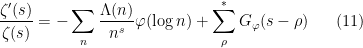
From (11) we have

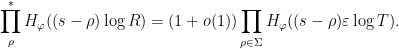
and we can integrate this to obtain

at least when the real part of is large enough (and we choose branches of  and
and  to vanish at ); one can justify the interchange of summation and integration using (13) (and the fact that is of order ). We can then exponentiate to conclude the formula

for  sufficiently large (where the factor at the pole
  is
is  due to the negative multiplicity); the right-hand side extends meromorphically to the entire complex plane, so (14) in fact holds for all
  .
.
Rescaling  to
to  (which rescales to
  ) for any
  , we obtain the generalisation

for all . While this formula is valid in the entire complex plane (other than the pole ), it is most useful to the right of the critical line, where most of the  factors become close to thanks to (13).
— 2. A microscale zero-free region —
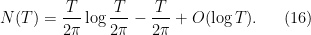
Let  denote the non-trivial zeroes of zeta (counting multiplicity), and let
  denote the number elements of with
  . The Riemann-von Mangoldt formula then gives the asymptotic
For any  , let
, let  denote the number of elements of with
  and . Clearly
  . The Riemann hypothesis asserts that
  . The Density hypothesis (in the log-free form) asserts the weaker bound that

This remains open; however bounds of the form

are known unconditionally for some . This was first achieved by Selberg for  , by Jutila for any
  , and by Conrey for any
  . However, for our analysis any positive value of will suffice.
As a corollary of (17) (and (16)), we see that for any  , there are
  zeroes
  with
with  and
and  . If we denote this set of zeroes by
  , then by the Hardy-Littlewood maximal inequality (applied to the sum of Dirac masses at the imaginary parts of these zeroes), for any
  , the event

holds with probability 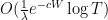 . Setting
  and then taking the union bound over
  that are powers of two, we conclude that with probability , one has

for all  and all that are a power of two. From this, (16), and renormalising
  , we thus have with probability that

for all  and
and  .
.
A similar argument (using the Riemann-von Mangoldt formula) shows that with probability , one has

for all (in fact one could replace  here by any other quantity that goes to infinity). We will improve this bound later (after discarding another exceptional event of ‘s).
Henceforth we restrict to the event that (18), (19) both hold. Since the left-hand side of (18) cannot go below one without vanishing entirely, we now have a “microscale” zero-free region
(say) for the Riemann zeta function. If we define the rescaled zero set

then we can rescale (18), (19) to be

for all and , and

for all  .
.
After shrinking the region a little bit, we have a quite precise formula for in this region:
Proposition 4 If  lies in the region
and  , then

for some absolute constant  . (We allow implied constants to depend on .)
Proof: We apply (15) with  . We have

and

for all  , so
, so
To evaluate the product, we write  , so that

We first consider those rescaled zeroes for which  . Here we see from (13) and the triangle inequality that

which we can then multiply using (22) and dyadic decomposition to conclude that

Now consider those for which  for some
  . Here we see from (13) that

for any  . Multiplying this using (21) and dyadic decomposition, we conclude for
  large enough that

Putting all this together, we conclude (23).
From the Cauchy integral formula one then has the bound
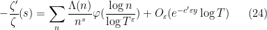
for all in the region

We can use the moment method to control the right-hand side of (24).
Proposition 5 Let  be fixed. With probability , one has the bound

for all in the region

One could improve the  loss here somewhat, in the spirit of the law of the iterated logarithm, but we will not attempt to do so here.
Proof: We can tile the region (25) by squares of the form

for various and  . By the union bound, it will suffice to show the bound

with probability  (say) for each such square
  , after restricting to the event that Proposition 4. Taking
  , it then suffices by that proposition to show that

with probability  , where
Let  be a large fixed even integer depending on
  .
.

where  is Lebesgue measure on . By linearity of expectation and Markov’s inequality, it then suffices to establish the bounds

and

uniformly for  . But this is a routine moment calculation (after first restoring the exceptional events in which (19), (22) fail in order to more easily compute the moment).
— 3. Microscale Riemann-von Mangoldt formulae —
Henceforth we restrict attention to the probability event where (19), (22), and Proposition 5 all hold. Then we have a microscale zero-free region slightly to the right of the critical line with good bounds on the log-derivative; by the functional equation, we also have good bounds slightly to the left of the critical line. Meanwhile, (19), (22) gives some preliminary control between these two lines. One can then put all this information together by standard techniques to obtain a microscale version of the Riemann-von Mangoldt formula, which we can then use to establish Theorem 2.
We turn to the details. We start from the well known identity

(see e.g., equation (45) of this previous blog post) for an absolute constant  and all
  that are not zeroes or poles of . In particular we have

On the other hand, from the functional equation (5) one has
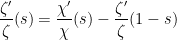
and hence

so that
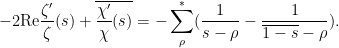
Writing and using (7), (20) we conclude

Using the functional equation we can replace  here by
  , and conclude that

In particular from Proposition 5 and writing  one has

when one is in the region (25) with  . The zeroes of imaginary part less than
  give a positive contribution to the LHS (which is comparable to
  when
when  , while the contributions of the zeroes of imaginary part greater than or equal to is
  for some
  thanks to (18). We conclude in particular the crude estimate

whenever one is in the region (25) with . If we then go back to (27) and integrate it for  in an interval
  in
in ![{[-e^{-cy/16}, e^{cy/16}]}](https://s0.wp.com/latex.php?latex=%7B%5B-e%5E%7B-cy%2F16%7D%2C+e%5E%7Bcy%2F16%7D%5D%7D&bg=ffffff&fg=000000&s=0&c=20201002) and use (28) to control errors, we conclude that
and use (28) to control errors, we conclude that

In particular, if we arrange the sort the rescaled zeroes  in nondecreasing order of real part, with
  for
for  and
and  for
for  , and such that any conjugate pairs of zeroes are consecutive, then we have the microscale Riemann-von Mangoldt formula

for  (as can be seen by applying the above formula with
 ![{I = [0,x]}](https://s0.wp.com/latex.php?latex=%7BI+%3D+%5B0%2Cx%5D%7D&bg=ffffff&fg=000000&s=0&c=20201002) or
or ![{I = [-x,0]}](https://s0.wp.com/latex.php?latex=%7BI+%3D+%5B-x%2C0%5D%7D&bg=ffffff&fg=000000&s=0&c=20201002) for
for  near
near  and
and  . Likely the error term can be improved with further effort. For
  one can also get very good control on
  from the classical Riemann-von Mangoldt formula.
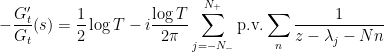
From (26) we have
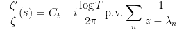
for some constant  depending on but not on , where we use (29) (and the classical Riemann-von Mangoldt formula) to ensure convergence of the principal value summation. If we set
  for some
  then from (29) we have

while from Proposition 5 one has

and hence  . Optimising in
  we thus have
  (say), hence

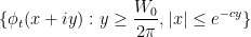
Next, let  be a consecutive string of rescaled zeroes in
  with
with  . By adjusting by one if necessary, we can assume that there are exactly zeroes in this string and that whenever one complex zero is in this set, its complex conjugate is also. Then we can define a degree polynomial

for some non-zero constant to be chosen later. This polynomial obeys a functional equation

for some phase  (which at present need not be equal to
  , but we will address this issue later). If we set
then  is an entire function, and from the Euler product formula for sine we have
whenever . Thus if we factor  , then by using (29) one can compute that

if  . Thus,
  only fluctuates by
  in this region. By choosing the normalising constant appropriately, one may thus ensure that
  in this region, thus giving the approximation (4) when . From (5) one thus has

when . From (8) one has

and thus

for at least one choice of . Thus the phase in (30) differs from by  (after shifting by an integer). Thus by adjusting the normalising constant by a multiplicative factor of
  , we obtain (9) as required.


29 comments
Comments feed for this article
4 May, 2019 at 7:18 am
Anonymous
The local trigonometric polynomial approximation to should be a good example for large x (for which
  zeros “solidify” to be very close to the zeros of a trigonometric polynomial), is it possible to generalize this to L- functions (or even to a larger class of Dirichlet series)?
4 May, 2019 at 1:06 pm
JDM
is there any way to turn these theoretical results about the zeta function into arithmetically useful information?
6 May, 2019 at 6:50 am
Terence Tao
Well, certainly many existing results and conjectures about the zeta function can be phrased in this framework, where they become marginally cleaner. For instance, one can establish the Selberg central limit theorem using this formalism: by pushing the analysis in this post a bit further, one can extract a factorisation
where and
and  is a polynomial which is “bounded in probability” in some sense (it is determined more or less completely by the nearby zeroes of zeta). The first factor has an asymptotically log-normal distribution and dominates the second factor (in probability) at say
  , which gives the Selberg central limit theorem. Conjecturally,
  should essentially be the characteristic polynomial of a random unitary matrix distributed using Haar measure, which would give the GUE hypothesis (and also 100% of zeroes on the critical line), and also predicts things like the moment and ratio conjectures for the Riemann zeta function.
9 May, 2019 at 12:27 pm
Anonymous
Study the harmonic series since it’s a prime source of prime number theory in regards to the Riemann Hypothesis and the Prime Number Theorem. Gauss and Riemann applied some tools of real analysis and complex analysis, respectively, to the harmonic series to achieve some great results.
Too much esoteric theory (above) is beside the point — it’s fancy mathematics which may lead one astray…
6 May, 2019 at 7:58 am
Anonymous
Is the Riemann Hypothesis true?
7 May, 2019 at 8:53 am
Anonymous
Hmm. Let’s take a poll. (It does not require a RH proof here.)
Press ‘Thumb Up’ Button to indicate a ‘Yes’ answer.
Press ‘Thumb Down’ Button to indicate a ‘No’ answer.
8 May, 2019 at 12:06 pm
Anonymous
Hints: A nontrivial zeta zero off the critical line (Re(z) = 1/2) does not make any sense. There’s no good reason for it. And it’s pure fiction or fake news too think otherwise.
9 May, 2019 at 9:44 am
Anonymous
Yes! Any attempt to refute the famous and important Riemann Hypothesis, Re(z_n) = 1/2, is a very futile exercise since the hypothesis is true! Please do something worthwhile.
And I can give you n (from one to infinity) reasons why the Riemann Hypothesis is true! Amen!
Moreover, it is unsound (incomplete) to discuss the properties of the nontrivial and simple zeta zeros of the Riemann Zeta Function without discussing the properties of primes.
They are are interdependent or interrelated. Amen!
Note: The nth nontrivial and simple zeta zero exists if and only if the nth prime exists.
13 May, 2019 at 10:32 am
Anonymous
Since my work in mathematics has brought me no happiness nor awards, I have decided to retire from it today…
Goodbye and good luck to all,
David Cole,
https://www.researchgate.net/profile/David_Cole29
22 May, 2019 at 1:42 pm
Anonymous
Keywords: Fundamental Theorem of Arithmetic and the Riemann Hypothesis
Basic and Important Fact Confirming RH (Riemann Hypothesis or Right Hypothesis, Re(z) = 1/2) where z is any nontrivial and simple zero of the Riemann Zeta Function:
For all n > 1, where n is any positive composite number, there exists a prime number, p, such that p|n (p divides n) where p ≤ n^(1/2) (p is less than or equal to the square root of n).
And thus, the exponent of of the expression, n^(1/2), which is 1/2 represents the critical line (Re(z) = 1/2) and confirms RH. And in turn, RH confirms the above basic and important fact. Amen!
The Riemann Hypothesis or the Right Hypothesis is true! Please acknowledge that fact!
David Cole.
Relevant Reference Link:
https://www.math10.com/forum/viewtopic.php?f=63&t=1549
P.S. I cannot retired from mathematics in peace while there are ‘experts’
of RH who claimed RH is still a open problem. They are either in denial or they do not understand RH!
.
27 June, 2019 at 4:45 pm
Anonymous
I made some harsh/ignorant comments below…, and I apologize. I wish everyone the best. David Cole.
6 May, 2019 at 3:29 pm
Joseph
About a local approximation of by trigonometric polynomials, I have thought about the following expression, for any
  :
:
which approximate the Riemann-Siegel function with an error
  for
for ![t \in [t_0 - t_0^{1/4}, t_0 + t_0^{1/4}]](https://s0.wp.com/latex.php?latex=t+%5Cin+%5Bt_0+-+t_0%5E%7B1%2F4%7D%2C+t_0+%2B+t_0%5E%7B1%2F4%7D%5D&bg=ffffff&fg=545454&s=0&c=20201002) (a consequence of the Riemann-Siegel formula, after linearizing the Riemann-Siegel theta function around
(a consequence of the Riemann-Siegel formula, after linearizing the Riemann-Siegel theta function around  ).
). on the real line, in function of
  . I don’t know if there are sufficiently convenient and powerful tools to study that. A few numerical simulations suggested me that most of the zeros of
  are on the real line for
  close to
  (where
  approximates
  well), but not for
  far from
  , except for values of
  such that he sum defining
  has one or two terms.
I have been curious about the behavior of the asymptotic proportion of zeros
8 May, 2019 at 5:42 am
Anonymous
Suppose that is allowed to be a quadratic polynomial in
  , is there an optimal coefficient (which may depend on
  ) of
) of  ?
?
8 May, 2019 at 11:28 am
Terence Tao
Right now describes a linear change of variables between the global coordinate
  and a “microscale” coordinate
  , which one can then convert nonlinearly to the coordinate
  . Both coordinates have some convenient features: in the microscale coordinate
  , the critical line is the real line (and the symmetry is reflection around that line), and in the nonlinear coordinate
  the critical line is now the unit circle (and the symmetry is the usual inversion across that circle). In the spirit of the Riemann mapping theorem one could consider a conformal change of coordinates to make the critical line some other Jordan curve, but it’s hard to imagine any of these being any more tractable than the line or circle, given how well understood the half-plane and disk domains are in complex analysis.
10 May, 2019 at 8:37 am
The alternative hypothesis for unitary matrices | What's new
[…] a recent post I discussed how the Riemann zeta function can be locally approximated by a polynomial, in the […]
15 May, 2019 at 7:52 am
Anonymous
Are these new results (especially Proposition 5) ? It seems quite strong.
15 May, 2019 at 8:54 am
Terence Tao
The basic tool powering these results – the zero density theorems of Selberg, Jutlia, and Conrey near the critical line – are not new, but I haven’t seen this application of these theorems in the prior literature. It was already known that these theorems tell us that “most” of the zeroes of zeta lie within of the critical line, giving a reasonable substitute for RH near a generic height
  ; the calculations here carry this sort of “near-RH on average” a bit further, giving a number of results of comparable strength to RH at generic heights. For instance there is also a prime number theorem for partial sums of
  with RH-like error term that one could get from Proposition 5 and Perron’s formula, though I didn’t write it down explicitly here.
15 May, 2019 at 8:38 am
Anonymous
Is it possible to combine theorem 2 and the probabilistic method to establish certain deterministic structures among consecutive zeta zeros on sufficiently short intervals?
15 May, 2019 at 8:56 am
Terence Tao
Possibly, if one also was able to get further information on the polynomial . Certainly for instance one can reinterpret existing results regarding the proportion of zeroes on the critical line, or bounds on the smallest or largest gap between zeroes, using this language, and viewing various known mean value theorems and moment theorems for the zeta function and related Dirichlet series as probabilistic estimates on
  (or on the log derivative of
  , or on moments of the zeroes, etc.)
17 May, 2019 at 8:53 am
A function field analogue of Riemann zeta statistics | What's new
[…] is another sequel to a recent post in which I showed the Riemann zeta function can be locally approximated by a polynomial, in the […]
25 May, 2019 at 1:41 pm
Anonymous
Are these polynomial approximations related to the Jensen polynomials being discussed in that paper making the news recently? https://www.pnas.org/content/early/2019/05/20/1902572116
Have you read it? Could you comment on the significance of their findings and maybe on the if and how of it relating to the things you’ve been looking at with respect to the RH?
25 May, 2019 at 3:29 pm
Terence Tao
I don’t see any connection. The approximations in this post are to the Riemann zeta function in a region at large height in the critical strip. The polynomials in that paper are constructed instead out of a (smoothed out) Taylor approximation of a high derivative of the Riemann xi function (with poles removed) at the central point
  . In this regime there does not seem to be a strong influence of either the zeroes of zeta or the rational primes, which are of course the two aspects of the zeta function that are of most importance in analytic number theory., and as a consequence the authors are able to get quite strong asymptotics in this regime.
29 May, 2019 at 11:36 am
Sunkhirous
Roots are all on Zero line S = 0+- i(pi +2kpi)/lnP^2^n , P is Prime pi =3.14… It’s sad that every mathematician trying to prove they lie on 1/2 line where don’t even know the exact value of these zeros , XI function have 1/2
29 May, 2019 at 12:33 pm
Anonymous
Sunkhirous, is that a formula for the nontrivial zeros of the Riemann zeta function?
29 May, 2019 at 12:35 pm
Anonymous
Yes
29 May, 2019 at 12:38 pm
Sunkhirous
i is for imaginary for S in the formula
29 May, 2019 at 2:32 pm
Sunkhirous
i = -1^.5
30 May, 2019 at 6:07 am
Anonymous
How are k, P, and n related to each other?
31 May, 2019 at 4:13 pm
Sunkhirous
k = 0,1,2,3…. n= 0,1,2… use k=0 for Riemann f(x) function