I’ve just uploaded to the arXiv my paper “Almost all Collatz orbits attain almost bounded values“, submitted to the proceedings of the Forum of Mathematics, Pi. In this paper I returned to the topic of the notorious Collatz conjecture (also known as the  conjecture), which I previously discussed in this blog post. This conjecture can be phrased as follows. Let
  denote the positive integers (with
  the natural numbers), and let
  be the map defined by setting
  equal to
  when
when  is odd and
  when is even. Let
  be the minimal element of the Collatz orbit
  . Then we have
Conjecture 1 (Collatz conjecture) One has  for all
  .
.
Establishing the conjecture for all remains out of reach of current techniques (for instance, as discussed in the previous blog post, it is basically at least as difficult as Baker’s theorem, all known proofs of which are quite difficult). However, the situation is more promising if one is willing to settle for results which only hold for “most” in some sense. For instance, it is a result of Krasikov and Lagarias that

for all sufficiently large  . In another direction, it was shown by Terras that for almost all (in the sense of natural density), one has
  . This was then improved by Allouche to
  for almost all and any fixed
  , and extended later by Korec to cover all
  . In this paper we obtain the following further improvement (at the cost of weakening natural density to logarithmic density):
Theorem 2 Let  be any function with
  . Then we have
  for almost all (in the sense of logarithmic density).
Thus for instance one has  for almost all (in the sense of logarithmic density).
The difficulty here is one usually only expects to establish “local-in-time” results that control the evolution  for times
  that only get as large as a small multiple
  of
of  ; the aforementioned results of Terras, Allouche, and Korec, for instance, are of this type. However, to get all the way down to
  one needs something more like an “(almost) global-in-time” result, where the evolution remains under control for so long that the orbit has nearly reached the bounded state
  .
.
However, as observed by Bourgain in the context of nonlinear Schrödinger equations, one can iterate “almost sure local wellposedness” type results (which give local control for almost all initial data from a given distribution) into “almost sure (almost) global wellposedness” type results if one is fortunate enough to draw one’s data from an invariant measure for the dynamics. To illustrate the idea, let us take Korec’s aforementioned result that if  one picks at random an integer from a large interval
 ![{[1,x]}](https://s0.wp.com/latex.php?latex=%7B%5B1%2Cx%5D%7D&bg=ffffff&fg=000000&s=0&c=20201002) , then in most cases, the orbit of will eventually move into the interval
, then in most cases, the orbit of will eventually move into the interval ![{[1,x^{\theta}]}](https://s0.wp.com/latex.php?latex=%7B%5B1%2Cx%5E%7B%5Ctheta%7D%5D%7D&bg=ffffff&fg=000000&s=0&c=20201002) . Similarly, if one picks an integer
. Similarly, if one picks an integer  at random from
 ![{[1,x^\theta]}](https://s0.wp.com/latex.php?latex=%7B%5B1%2Cx%5E%5Ctheta%5D%7D&bg=ffffff&fg=000000&s=0&c=20201002) , then in most cases, the orbit of will eventually move into
, then in most cases, the orbit of will eventually move into ![{[1,x^{\theta^2}]}](https://s0.wp.com/latex.php?latex=%7B%5B1%2Cx%5E%7B%5Ctheta%5E2%7D%5D%7D&bg=ffffff&fg=000000&s=0&c=20201002) . It is then tempting to concatenate the two statements and conclude that for most in , the orbit will eventually move . Unfortunately, this argument does not quite work, because by the time the orbit from a randomly drawn
. It is then tempting to concatenate the two statements and conclude that for most in , the orbit will eventually move . Unfortunately, this argument does not quite work, because by the time the orbit from a randomly drawn ![{N \in [1,x]}](https://s0.wp.com/latex.php?latex=%7BN+%5Cin+%5B1%2Cx%5D%7D&bg=ffffff&fg=000000&s=0&c=20201002) reaches , the distribution of the final value is unlikely to be close to being uniformly distributed on , and in particular could potentially concentrate almost entirely in the exceptional set of
reaches , the distribution of the final value is unlikely to be close to being uniformly distributed on , and in particular could potentially concentrate almost entirely in the exceptional set of ![{M \in [1,x^\theta]}](https://s0.wp.com/latex.php?latex=%7BM+%5Cin+%5B1%2Cx%5E%5Ctheta%5D%7D&bg=ffffff&fg=000000&s=0&c=20201002) that do not make it into . The point here is the uniform measure on is not transported by Collatz dynamics to anything resembling the uniform measure on .
that do not make it into . The point here is the uniform measure on is not transported by Collatz dynamics to anything resembling the uniform measure on .
So, one now needs to locate a measure which has better invariance properties under the Collatz dynamics. It turns out to be technically convenient to work with a standard acceleration of the Collatz map known as the Syracuse map  , defined on the odd numbers
  by setting
  , where
  is the largest power of
  that divides . (The advantage of using the Syracuse map over the Collatz map is that it performs precisely one multiplication of
  at each iteration step, which makes the map better behaved when performing “-adic” analysis.)
When viewed -adically, we soon see that iterations of the Syracuse map become somewhat irregular. Most obviously,  is never divisible by . A little less obviously, is twice as likely to equal mod as it is to equal
  mod . This is because for a randomly chosen odd
  , the number of times
  that divides
  can be seen to have a geometric distribution of mean – it equals any given value
  with probability
  . Such a geometric random variable is twice as likely to be odd as to be even, which is what gives the above irregularity. There are similar irregularities modulo higher powers of . For instance, one can compute that for large random odd ,
  will take the residue classes
  with probabilities
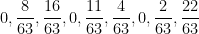
respectively. More generally, for any ,  will be distributed according to the law of a random variable
  on
on  that we call a Syracuse random variable, and can be described explicitly as

where  are iid copies of a geometric random variable of mean .
In view of this, any proposed “invariant” (or approximately invariant) measure (or family of measures) for the Syracuse dynamics should take this -adic irregularity of distribution into account. It turns out that one can use the Syracuse random variables to construct such a measure, but only if these random variables stabilise in the limit  in a certain total variation sense. More precisely, in the paper we establish the estimate


for any  and any
  . This type of stabilisation is plausible from entropy heuristics – the tuple
  of geometric random variables that generates has Shannon entropy
  , which is significantly larger than the total entropy
  of the uniform distribution on , so we expect a lot of “mixing” and “collision” to occur when converting the tuple to ; these heuristics can be supported by numerics (which I was able to work out up to about
  before running into memory and CPU issues), but it turns out to be surprisingly delicate to make this precise.
A first hint of how to proceed comes from the elementary number theory observation (easily proven by induction) that the rational numbers

are all distinct as  vary over tuples in
  . Unfortunately, the process of reducing mod
  creates a lot of collisions (as must happen from the pigeonhole principle); however, by a simple “Lefschetz principle” type argument one can at least show that the reductions

are mostly distinct for “typical”  (as drawn using the geometric distribution) as long as
  is a bit smaller than
  (basically because the rational number appearing in (3) then typically takes a form like
  with an integer between
  and ). This analysis of the component (3) of (1) is already enough to get quite a bit of spreading on
  (roughly speaking, when the argument is optimised, it shows that this random variable cannot concentrate in any subset of of density less than
  for some large absolute constant
  ). To get from this to a stabilisation property (2) we have to exploit the mixing effects of the remaining portion of (1) that does not come from (3). After some standard Fourier-analytic manipulations, matters then boil down to obtaining non-trivial decay of the characteristic function of , and more precisely in showing that

for any and any  that is not divisible by .
If the random variable (1) was the sum of independent terms, one could express this characteristic function as something like a Riesz product, which would be straightforward to estimate well. Unfortunately, the terms in (1) are loosely coupled together, and so the characteristic factor does not immediately factor into a Riesz product. However, if one groups adjacent terms in (1) together, one can rewrite it (assuming is even for sake of discussion) as


where  . The point here is that after conditioning on the
  to be fixed, the random variables
  remain independent (though the distribution of each
  depends on the value that we conditioned
  to), and so the above expression is a conditional sum of independent random variables. This lets one express the characeteristic function of (1) as an averaged Riesz product. One can use this to establish the bound (4) as long as one can show that the expression

is not close to an integer for a moderately large number ( , to be precise) of indices
  . (Actually, for technical reasons we have to also restrict to those
  for which
  , but let us ignore this detail here.) To put it another way, if we let
  denote the set of pairs
  for which
![\displaystyle \frac{\xi 3^{2j-2} (2^{-l+1} \mod 3^n)}{3^n} \in [-\varepsilon,\varepsilon] + {\bf Z},](https://s0.wp.com/latex.php?latex=%5Cdisplaystyle++%5Cfrac%7B%5Cxi+3%5E%7B2j-2%7D+%282%5E%7B-l%2B1%7D+%5Cmod+3%5En%29%7D%7B3%5En%7D+%5Cin+%5B-%5Cvarepsilon%2C%5Cvarepsilon%5D+%2B+%7B%5Cbf+Z%7D%2C+&bg=ffffff&fg=000000&s=0&c=20201002)
we have to show that (with overwhelming probability) the random walk

(which we view as a two-dimensional renewal process) contains at least a few points lying outside of .
A little bit of elementary number theory and combinatorics allows one to describe the set as the union of “triangles” with a certain non-zero separation between them. If the triangles were all fairly small, then one expects the renewal process to visit at least one point outside of after passing through any given such triangle, and it then becomes relatively easy to then show that the renewal process usually has the required number of points outside of . The most difficult case is when the renewal process passes through a particularly large triangle in . However, it turns out that large triangles enjoy particularly good separation properties, and in particular afer passing through a large triangle one is likely to only encounter nothing but small triangles for a while. After making these heuristics more precise, one is finally able to get enough points on the renewal process outside of that one can finish the proof of (4), and thus Theorem 2.


480 comments
Comments feed for this article
31 August, 2021 at 9:16 am
Wulf Rehder
Calculating the Total Stopping Time N(T):
[Note: In my last reply of August 29, above, the final sentence has a typo: “ratio (m+k)^N” should read “ratio (m+k)/N”.]
My previous comments on the Collatz Conjecture in this thread have shown that the stopping time N=N(S) can be determined by the proportion of divisions by 2 and the constant t, which is related to the Cantor fractal dimension r=log2/log3 or, equivalently, to the Sierpinski fractal dimension s=1/r, by the relationship t=1/(r+1)=s/(s+1)=0.613147…. To wit: If m is the number of multiplications by 3 and m+k the number of divisions by 2 up to the index N=m+m+k, then N=N(S) is the stopping time of this sequence iff at this N the proportion
(*) (m+k)/N >= t for the first time.
The starting element c(0) (the “seed”) of the Collatz sequence does not explicitly appear in this formula. This characterization of the stopping time in terms of a fractal dimension has been verified with all available data, for instance https://en.wikipedia.org/wiki/Collatz_conjecture#Empirical_data as well as for the Collatz-relevant sequences A006884 and A006577 in the OEIS.
In a similar way, the total stopping time N(T), the index at which the Collatz sequence hits down to 1, can be characterized in terms of s, r, and t. Here, however, the seed c(0) figures explicitly. Again we are looking for the excess k of the number of divisions by 2 over the number m of multiplications by 3, such that this excess pushes the seed c(0) down to 1:
(**) c(0) 3^m/2^(m+k) N(S) and
(***) [k+m-log(c(0))/log2]/[N-log(c(0))/log2] >= t,
with t being the threshold defined above.
Comparing (***) to (*) shows how the seed c(0) enters the calculation of the total stopping time explicitly. [N(T)>N(S) is added because for some small N=1,2,3, … = C, or (k+m)-sm >= D,
with C>0 and D>0 depending on the seed c(0): The Collatz sequence with seed c(0) reaches 1 after m+m+k steps, iff the relationship between the m+k divisions by 2 and the m multiplications by 3 are given by the fractal dimensions r and s in (****).
None of this proves the Collatz Conjecture, of course. However, the somewhat elusive conjecture “The sequence eventually reaches 1” can be more concretely expressed in terms of the inequalities (***) or (****). A counter-example to the Collatz Conjecture would require a seed c(0) such that, for instance, r(k+m)-m < C for all N=m+m+k..
P.S.: A reader who intends to “Rate Down” this or any other post – which seems to happen almost automatically in this thread, quite drastically even for contributions by Dr. Tao – is politely requested to give a reason in a reply, or better even, a counter-example. I’d be happy to explain further. Thanks!
31 August, 2021 at 11:25 pm
Wulf Rehder
Calculating the Total Stopping Time N(T)
For mysterious reasons a part of the text was excised in the copy-paste process of the above posting: Instead of the text from “Comparing (***) to (*) …” and “… r and s in (****)” the correct text should read:
“Comparing (***) to (*) shows how the seed c(0) enters the calculation of the total stopping time explicitly. [N(T)>N(S) is added because for some small N=1,2,3, … = C, or (k+m)-sm >= D,
with C>0 and D>0 depending on the seed c(0): The Collatz sequence with seed c(0) reaches 1 after m+m+k steps, iff the relationship between the m+k divisions by 2 and the m multiplications by 3 are given by the fractal dimensions r and s in (****).”
31 August, 2021 at 11:43 pm
Wulf Rehder
Calculating the Total Stopping Time N(T)
I found the mysterious reason: There was a “smaller than” symbol in the text, which is fatal in certain versions of wordpress. Now then: Instead of the text from “Comparing (***) to (*) …” and “… r and s in (****)” the correct text should read:
“Comparing (***) to (*) shows how the seed c(0) enters the calculation of the total stopping time explicitly. [N(T)>N(S) is added because for some small N=1,2,3, … smaller than N(S) the ratio (***) may be large or even negative.] This too has been corroborated with a wide variety of interesting seeds c(0)=27, 97, 871, 6 171, 77 031, 837 799, … and OEIS sequences.
Defining the constants A=log(c(0))/log2, B=tA, (A-B)/t=C, D=C/r makes (***) more compact:
(****) r(k+m)-m >= C, or (k+m)-sm >= D,
with C>0 and D>0 depending on the seed c(0): The Collatz sequence with seed c(0) reaches 1 after m+m+k steps, iff the relationship between the m+k divisions by 2 and the m multiplications by 3 are given by the fractal dimensions r and s in (****).”
Sorry about this.
20 September, 2021 at 7:40 am
De Wi
Wulf Rehder, I am writing some code on Collatz Sequences on Tool Control Language, TCL. Thanks for your previous (TAO) posts on subject. Is there a “formula” or psuedocode steps to estimate the number of elements or steps of a Collatz Sequence before computing the Collatz Sequence by the computer. The complement to your Rehder_limt is 0.3868528072345415 or 38.6 percent. Might useful in some situations. Thank you.
Tool Control Language = TCL.
—————————————————-
proc collatz_sequences_Krasikov_Lagarias_limit {limit} {
if { $limit <= 1 } {
return -code error "The limit must be larger than 1"
}
expr {$limit** 0.84}
}
# Krasikov and Lagarias limit 4 3.204
# Krasikov and Lagarias limit 5 3.864
# Krasikov and Lagarias limit 10 6.918
# Krasikov and Lagarias limit 20 12.384
# Krasikov and Lagarias limit 50 26.738
set Rehder_limit_collatz_sequences [ return [ expr { (log(3)/log(2))/(log(3)/log(2)+1.)} ] ]
# returns 0.61314719276545848 or or 61.3 percent
set Rehder_limit_complement [ return [ expr { 1.- (log(3)/log(2))/(log(3)/log(2)+1.)} ] ]
# returns 0.3868528072345415 or 38.6 percent
20 September, 2021 at 8:04 am
michaelmross
There is the special case of 4n+1 being always a sequence with one more step than sequence n – really the same sequence with one earlier step. Now also remember, that the stopping time of every number in a sequence is known from the first number in the sequence. Every number can only be a member of one sequence.
Besides that there are nonrecursive functions – that is, ones that eliminate division or exponentiation, so they have linear running time, such as:
One may also consider the possibility that sequences are actually superfluous, and the conjecture concerns the finitude of the input and output of a table with three congruences and three operations. https://youtu.be/q1F50FTpg8A
7 February, 2023 at 7:07 pm
Andrew Croft
I have also produced the function michaelmross describes, working with the Syracuse sequence, as every step in a single iteration is tidy, which I prefer to dividing by 2 to a variable power, but I fail to see it contributing to the global question of everything going to 1.
Each step in the sequence depends on the behaviour of n mod 8, and when you iterate this function, it’s quite tidy provided n mod 8 is 3 or 7, but as soon as it switches to n mod 8 being 1 or 5, and then switches back, then the number of terms involves blows up … which is why the global problem is so hard.
An equivalent function can be produced for the 3n-1 problem with its 3 cycles, but this function doesn’t explain the 3 cycles vs the 1 for 3n+1, well not to me anyway.
Back to the drawing board and trying in my amateur way to understand Prof Tao’s papers.
22 September, 2021 at 7:14 am
De Wi
Subject: Possible Uses for Collatz Sequences Conjecture?
#### A novice programmer (me) has received offsite query from “senior programmer in charge” ..>>> .. ” While I am fascinated by the Collatz problem, I do not see much practical use for it. In what kind of computer applications would you use this?”
—————————
#### Answer, As understood here, the Collatz Sequences Conjecture is called pure mathematics. Paul Erdős said about the Collatz conjecture: “Mathematics may not be ready for such problems.” The Collatz Sequences Conjecture is at the forefront of human mathematics. From what an outsider can tell, the Collatz Sequences are being generated with supercomputers and distributed computing algoritms on the numeric issues. Apparently, the Collatz Sequences are as valid a test for computing machines, parallel algoritms, and distributed computing algoritms as the 1) search for pi , 2) search for highest prime number, 3) Twin Prime Conjecture, and 4) factoring numbers . The novice has written TCL hacks on all five subjects. In 2020, starting values up to 2**268 approximating 2.95*1020 have been checked in the Collatz conjecture. I suppose the question is valid, if one is advocating spending time, salaried employees, and resources on pure mathematics and the Collatz Sequences Conjecture to decision making nodes. .I am a retired engineer. Maybe the pure mathematicians among us may offer some more practical uses for the Collatz Sequences Conjecture?
Samples from Tool Control Language = TCL.
—————————————————-
proc collatz_sequences_Krasikov_Lagarias_limit {limit} {
if { $limit <= 1 } {
return -code error "The limit must be larger than 1"
}
expr {$limit** 0.84}
}
# Krasikov and Lagarias limit 4 3.204
# Krasikov and Lagarias limit 5 3.864
# Krasikov and Lagarias limit 10 6.918
# Krasikov and Lagarias limit 20 12.384
# Krasikov and Lagarias limit 50 26.738
set Rehder_limit_collatz_sequences [ return [ expr { (log(3)/log(2))/(log(3)/log(2)+1.)} ] ]
# returns 0.61314719276545848 or or 61.3 percent
set Rehder_limit_complement [ return [ expr { 1.- (log(3)/log(2))/(log(3)/log(2)+1.)} ] ]
# returns 0.3868528072345415 or 38.6 percent
19 October, 2021 at 3:50 pm
E F
Dear All,
Today I posted a document on Reddit regarding the Collatz conjecture (Family Tree Problem). I have tried to approach the Collatz conjecture in a different way with the idea of discovering new patterns. I have a strongly believe that the mathematical functions f(n) = 3n – 1, f(n) = 2n – 1, f(n) = 3n + 1 and f(n) = 4n + 1 are closely related to the Family Tree Anomalies (Loops related to f(n) = 3n + 1) especially for n = 0, n = -2, n = -6 and n = -8. Please take a look at it if you have any spare time these days.
I tried to copy some details of the document for you, but maybe the readability is not best.
Family Tree “Genealogy” Problem (Reverse Collatz Conjecture)
By EF
October 15, 2021
*THE MATHEMATICAL FUNCTIONS RELATED TO THE FAMILY TREE PROBLEM ARE:
f(n) = 3n + 1; to generate Parent of n
f(n) = n + [(n – 1) / 3]; to generate Child (firstborn) of n
f(n) = n – [(n + 1) / 3]; to generate Child (firstborn) of n
f(n) = 2n; to generate Child (firstborn) of n (n divisible by 3 doesn’t have any odd children)
f(n) = 4n + 1; to generate Sibling of n
f(m,n) = {[(4^(m-1)).(3n + 1)] – 1} / 3; to generate Birth order of e.g. Siblings or Children of n, where m = Birth order
*EXAMPLE PERSON N = 11
9 Grandchild ; f(9) = 2n = 18 (n divisible by 3 doesn’t have any odd
children)
x3 + 1 =
28 f(9) = 3n + 1
/2 =
14 f(9) = (3n + 1) / 2
/2 =
7 Child (firstborn) ; f(9) = ((3n + 1) / 2) / 2 ; f(11) = n – [(n + 1) / 3] = 7
(Firstborn of 11)
x3 + 1 =
22 f(7) = 3n + 1
/2 =
11 Person ; f(7) = (3n + 1) / 2 ; f(17) = n – [(n + 1) / 3] = 11 (Firstborn of 17)
x3 + 1 =
34 f(11) = 3n + 1
/2 =
17 Parent ; f(11) = (3n + 1) / 2 ; f(13) = n + [(n – 1) / 3] = 17 (Firstborn of 13)
x3 + 1 =
52 f(17) = 3n + 1
/2 =
26 f(17) = (3n + 1) / 2
/2 =
13 Grandparent ; f(17) = ((3n + 1) / 2) / 2 ;
f(2,5) = {[(4^(m-1)).(3n + 1)] – 1} / 3 = 13 (Second Child of 5)
x3 + 1 =
40 f(13) = 3n + 1
/2 =
20 f(13) = (3n + 1) / 2
/2 =
10 f(13) = ((3n + 1) / 2) / 2
/2 =
5 Great-Grandparent ; f(13) = (((3n + 1) / 2) / 2) / 2 ;
f(2,1) = {[(4^(m-1)).(3n + 1)] – 1} / 3 = 5 (Second Child of 1)
x3 + 1 =
16 f(5) = 3n + 1
/2 =
8 f(5) = (3n + 1) / 2
/2 =
4 f(5) = ((3n + 1) / 2) / 2
/2 =
2 f(5) = (((3n + 1) / 2) / 2) / 2
/2 =
1 Great-Great-Grandparent and Sibling of Great-Grandparent are the
same person (Parent and Firstborn Child are the same person)
f(5) = ((((3n + 1) / 2) / 2) / 2) / 2
x3 + 1 =
4 f(1) = 3n + 1
/2 =
2 f(1) = (3n + 1) / 2
/2 =
1 Progenitor (Founder of the Collatz family); 1 is Parent of Firstborn Child
1 and Grandparent of Firstborn Grandchild 1 (Parent and Firstborn
Child and Firstborn Grandchild are the same person namely 1)
f(1) = ((3n + 1) / 2) / 2
*EXAMPLE PERSON N = 11
f(m,n) = {[(4^(m-1)).(3n + 1)] – 1} / 3 ; Birth order of siblings or children of n ; where m = Birth Order
Siblings of 9 (Grandsons and Granddaughters of 11)
37 (second sibling); 149 (third sibling); 597 (fourth sibling); 2389 (fifth sibling) f(9) = 4n + 1
(m,n) = (1,9) = 9; (m,n) = (2,9) = 37; (m,n) = (3,9) = 149; (m,n) = (4,9) = 597; (m,n) = (5,9) = 2389
Siblings of 7 (Sons and Daughters of 11)
29 (second sibling); 117 (third sibling); 469 (fourth sibling); 1877 (fifth sibling) f(7) = 4n + 1
(m,n) = (1,7) = 7; (m,n) = (2,7) = 29; (m,n) = (3,7) = 117; (m,n) = (4,7) = 469; (m,n) = (5,7) = 1877
Siblings of 11 (Brothers and Sisters of 11)
45 (second sibling); 181 (third sibling); 725 (fourth sibling); 2901 (fifth sibling) f(11) = 4n + 1
(m,n) = (1,11)= 11; (m,n) = (2,11) = 45; (m,n) = (3,11) = 181; (m,n) = (4,11) = 725; (m,n) = (5,11) = 2901
Siblings of 17 (Aunts and Uncles of 11)
69 (second sibling); 277 (third sibling); 1109 (fourth sibling); 4437 (fifth sibling) f(17) = 4n + 1
(m,n) = (1,17) = 17; (m,n) = (2,17) = 69; (m,n) = (3,17) = 277; (m,n) = (4,17) = 1109; (m,n) = (5,17) = 4437
Siblings of 13 (Grandaunts and Granduncles of 11)
3 (first sibling); 53 (third sibling); 213 (fourth sibling); 853 (fifth sibling) f(13) = 4n + 1
(m,n) = (1,13) = 13; (m,n) = (2,13) = 53; (m,n) = (3,13) = 213; (m,n) = (4,13) = 853; (m,n) = (5,13) = 3413
(m,n) = (1,3) = 3; (m,n) = (2,3) = 13; (m,n) = (3,3) = 53; (m,n) = (4,3) = 213; (m,n) = (5,3) = 853
Siblings of 5 (Great-Grandaunts and Great-Granduncles of 11)
1 (first sibling); 21 (third sibling); 85 (fourth sibling); 341 (fifth sibling) f(5) = 4n + 1
(m,n) = (1,5) = 5; (m,n) = (2,5) = 21; (m,n) = (3,5) = 85; (m,n) = (4,5) = 341; (m,n) = (5,5) = 1365
(m,n) = (1,1) = 1; (m,n) = (2,1) = 5; (m,n) = (3,1) = 21; (m,n) = (4,1) = 85; (m,n) = (5,1) = 341
Siblings of 1
5 (second sibling); 21 (third sibling); 85 (fourth sibling); 341 (fifth sibling)
(m,n) = (1,1) = 1; (m,n) = (2,1) = 5; (m,n) = (3,1) = 21; (m,n) = (4,1) = 85; (m,n) = (5,1) = 341
The loops regarding f(n) = 3n + 1 can be explained as anomalies related to the Family Tree.
*LOOPS OF F(N) = 3N + 1 (ANOMALIES IN FAMILY TREES)
f(n) = 3n + 1 f(n) = n + [(n – 1) / 3] f(n) = n – [(n + 1) / 3] f(n) = 4n + 1
Parent of n Child (firstborn) of n Child (firstborn) of n Siblings of n
n = 1
4 1 5
/ 2 21
2 85
/ 2 341
1
1 is Parent of Firstborn Child 1 and Grandparent of Firstborn Grandchild 1 (Parent and Firstborn Child and Firstborn Grandchild are the same person namely 1)
n = -1
-2 -1 -3
/ 2 -11
-1 -43
-1 is Parent of Firstborn Child -1 and Grandparent of Firstborn Grandchild -1
(Parent and Firstborn Child and Firstborn Grandchild are the same person namely -1)
n = -5
-14 -7 -19
/ 2 -75
-7 -299
-7 is Parent of Firstborn Child -5 and Grandparent of Firstborn Grandchild -7 (Grandparent and Firstborn Grandchild are the same person namely -7)
n = -7
-20 -5 -27
/ 2 -107
-10 -427
/ 2
-5
-5 is Parent of Firstborn Child -7 and Grandparent of Firstborn Grandchild -5 (Grandparent and Firstborn Grandchild are the same person namely -5)
n = -23
-68 -31 (-23 is Firstborn and -91 is Second Child of -17) /2
-34 -91
/ 2 -363
-17 -1451
n = -17
-50 -23 (-17 is Parent of -23) -67
/ 2 -267
-25 -1067
n = -25
-74 (-25 is Parent of -17) -17 -99
/ 2 -395
-37 -1579
n = -37
-110 (-37 is Grandparent of -17) -25 -147
/ 2 -587
-55 -2347
n = -55
-164 -37 (-55 is Great-Grandparent of -17) -219
/ 2 -875
-82 -3499
/2
-41
n = -41
-122 -55 (-41 is Great-Great-Grandparent of -17)
/ 2 -163
-61 -651
-2603
n = -61
-182
/ 2
-91
-61 is Great-Great-Great-Grandparent of -17 and Great-Great-Great-Great-Grandparent of -91
-91 is Great-Great-Great-Great-Grandparent of -17 and Great-Great-Great-Great-Great-Grandparent of -91
-91 is Second Child of -17 and Great-Great-Great-Great-Grandchild of -61
(‘Great-Great-Great-Great-Great-Grandchild’ and ‘Great-Great-Great-Great-Great-Grandparent’ are the same person namely -91)
n = -91
-272
/ 2
-136
/ 2
-68
/ 2
-34
/ 2
-17
*THE FUNCTIONS F(N) = 3N – 1, F(N) = 2N – 1, F(N) = 3N + 1 AND F(N) = 4N + 1 ARE CLOSELY RELATED TO THE FAMILY TREE ANOMALIES (LOOPS RELATED TO F(N) = 3N + 1) ESPECIALLY FOR N = 0, N = -2, N = -6 AND N = -8.
The difference of P and C is n The difference of C and P is n
(3n -1) – (2n -1) = n (4n + 1) – (3n + 1) = n
Parent Child Parent Child
f(n) = 3n – 1 f(n) = 2n – 1 n f(n) = 3n + 1 f(n) = 4n + 1
-106 -71 -35 -104 -139
-103 -69 -34 -101 -135
-100 -67 -33 -98 -131
-97 -65 -32 -95 -127
-94 -63 -31 -92 -123
-91 -61 -30 -89 -119
-88 -59 -29 -86 -115
-85 -57 -28 -83 -111
-82 -55 -27 -80 -107
-79 -53 -26 -77 -103
-76 -51 -25 -74 -99
-73 -49 -24 -71 -95
-70 -47 -23 -68 -91
-67 -45 -22 -65 -87
-64 -43 -21 -62 -83
-61 -41 -20 -59 -79
-58 -39 -19 -56 -75
-55 -37 -18 -53 -71
-52 -35 -17 -50 -67
-49 -33 -16 -47 -63
-46 -31 -15 -44 -59
-43 -29 -14 -41 -55
-40 -27 -13 -38 -51
-37 -25 -12 -35 -47
-34 -23 -11 -32 -43
-31 -21 -10 -29 -39
-28 -19 -9 -26 -35
-25 -17 -8 -23 -31
-22 -15 -7 -20 -27
-19 -13 -6 -17 -23
-16 -11 -5 -14 -19
-13 -9 -4 -11 -15
-10 -7 -3 -8 -11
-7 -5 -2 -5 -7
-4 -3 -1 -2 -3
-1 -1 0 1 1
2 1 1 4 5
5 3 2 7 9
8 5 3 10 13
11 7 4 13 17
14 9 5 16 21
17 11 6 19 25
20 13 7 22 29
23 15 8 25 33
26 17 9 28 37
29 19 10 31 41
32 21 11 34 45
35 23 12 37 49
38 25 13 40 53
41 27 14 43 57
44 29 15 46 61
47 31 16 49 65
50 33 17 52 69
53 35 18 55 73
56 37 19 58 77
59 39 20 61 81
62 41 21 64 85
65 43 22 67 89
68 45 23 70 93
71 47 24 73 97
74 49 25 76 101
Intersection Point f(n) = 3n + 1 and f(n) = 4n + 1 (0 ; 1)
Intersection Point f(n) = 2n – 1 and f(n) = 3n + 1 (-2 ; -5)
Intersection Point f(n) = 2n – 1 and f(n) = 3n – 1 (0 ; -1)
Intersection Point f(n) = 3n – 1 and f(n) = 2n (1 ; 2)
Intersection Point f(n) = 3n + 1 and f(n) = 2n (-1 ; -2)
Intersection Point f(n) = 2n – 1 and f(n) = n + [(n – 1) / 3] (1 ; 1)
Intersection Point f(n) = 2n – 1 and f(n) = 4n + 1 (-1 ; -3)
Intersection Point f(n) = 2n – 1 and f(n) = n – [(n + 1) / 3] (0,5 ; 0)
Intersection Point f(n) = 4n + 1 and f(n) = 2n and f(n) = n + [(n – 1) / 3]
(-0,5 ; -1)
Intersection Point f(n) = n + [(n – 1) / 3] and f(n) = n – [(n + 1) / 3] (0 ; -1/3)
Intersection Point f(n) = 3n – 1 and f(n) = 4n + 1 (-2 ; -7)
Intersection Point f(n) = 3n – 1 and f(n) = n + [(n – 1) / 3] (2/5 ; 1/5)
N = 4
f(4) = 3n + 1 = 13 f(13) = 3n + 1 = 40 / 2 = 20 / 2 = 10 / 2 = 5
(5 is parent of 13)
f(4) = 4n + 1 = 17 f(17) = 3n + 1 = 52 / 2 = 26 / 2 = 13
(13 is parent of 17)
f(4) = 2n – 1 = 7 f(7) = 3n + 1 = 22 / 2 = 11 (11 is parent of 7)
f(4) = 3n – 1 = 11 f(11) = 3n + 1 = 34 / 2 = 17 (17 is parent of 11)
7 x 3 + 1 = 22 / 2 = 11 x 3 + 1 = 34 / 2 = 17 x 3 + 1 = 52 / 2 = 26 / 2 = 13 x 3 + 1 = 40 / 2 = 20 / 2 = 10 / 2 = 5
13 is Great-Grandparent of 7
17 is Grandparent of 7
11 is Parent of 7
N = -8
f(-8) = 4n + 1 = -31 f(-31) = 3n + 1 = -92 / 2 = -46 / 2 = -23
-23 is parent of -31 (-31 is Grandchild of -17)
f(-8) = 3n + 1 = -23 f(-23) = 3n + 1 = -68 / 2 = -34 / 2 = -17
-17 is parent of -23 (-23 is child of -17)
f(-8) = 2n – 1 = -17 f(-17) = 3n + 1 = -50 / 2 = -25
-25 is Parent of -17 (-25 is parent of -17)
f(-8) = 3n – 1 = -25 f(-25) = 3n + 1 = -74 / 2 = -37
-37 is Parent of -25 (-37 is Grandparent of -17)
-31 x 3 + 1 = -92 / 2 = -46 / 2 = -23 x 3 + 1 = -68 / 2 = -34 / 2 = -17 x 3 + 1 = -50 / 2 = -25 x 3 + 1 = -74 / 2 = -37
N = -6 N = -8
f(-6) = 4n + 1 = -23 f(-8) = 3n + 1 = -23
-23 is Child of -17 -23 is Child of -17
f(-6) = 3n + 1 = -17 f(-8) = 2n – 1 = -17
(3n -1) – (2n -1) = 0 and n = 0 (4n + 1) – (3n + 1) = 0 and n = 0
-1 – -1 = 0 1 – 1 = 0
n = -1 n = 1
-2 4
-1 2
-2 1
-1 4
2
1
(3n -1) – (2n -1) = -2 and n = -2 (4n + 1) – (3n + 1) = -2 and n = -2
-7 – -5 = -2 -7 – -5 = -2
n = -5 n = -7
-14 -20
-7 -10
-20 -5
-10 -14
-5 -7
-14 -20
-7 -10
-20 -5
-10 -14
-5 -7
(3n -1) – (2n -1) = -8 (4n + 1) – (3n + 1) = -8 (4n + 1) – (3n + 1) = -6
and n = -8 and n = -8 and n = -6
-25 – -17 = -8 -31 – -23 = -8 -23 – -17 = -6
n = -31 n = -31 n = -31
-92 -92 -92
-46 -46 -46
-23 -23 -23
-68 -68 -68
-34 -34 -34
-17 -17 -17
-50 -50 -50
-25 -25 -25
-74 -74 -74
-37 -37 -37
-110 -110 -110
-55 -55 -55
-164 -164 -164
-82 -82 -82
-41 -41 -41
-122 -122 -122
-61 -61 -61
-182 -182 -182
-91 -91 -91
-272 -272 -272
-136 -136 -136
-68 -68 -68
-34 -34 -34
-17 -17 -17
MISCELLANEOUS:
*f(-0,5) = 3 x -0,5 + 1 = -0,5 (shortest loop).
*1 is the only positive integer that fulfill three different roles namely Parent, Firstborn Child and Firstborn Grandchild as well and thus ends in a vicious circle (1-4-2-1 loop).
*If it can be proven that the existing loops mentioned above (1 ; 1), (-1 ; -1), (-5 ; -7, -7 ; -5) and (-23 ; -17) are the only 4 anomalies related to the Family Tree Problem, f(n) = 3n + 1, then the Collatz Conjecture is true.
20 October, 2021 at 12:06 pm
Anonymous
Any (valid) proof of the Collatz conjecture must use new(!) methods.
21 October, 2021 at 10:06 pm
Gaurav Krishna
Here is the proof for Collatz Conjecture
https://vixra.org/abs/2110.0119
#Collatz #3n+1
27 November, 2021 at 1:18 pm
Anonymous
can I get a good email contact for someone who has studied this conjecture , I think I might have an idea.
1 December, 2021 at 6:37 am
sacirisi
With the Collatz algorithm it is not possible to process all natural numbers because we do not know: quantities and values of even and odd numbers and all their factors. From Tartaglia’s triangle we can detect odd numbers which are the sum of the results of the infinite powers of 2 which have an even index and which are also equal to the previous odd * 4 + 1. These are all the odd numbers that * 3 + 1 generate an even number that is the result of a base power 2 and even index 2 ^ (2 * n≥1) and that, the nth half, ends at 1 because ½ of 2 ^ 1 = 2 ^ 0 = 1. https://www.facebook.com/groups/5349868060/my_posted_content
29 December, 2021 at 7:23 pm
Anonymous
Collatz value-dropping formulas:
If the first lower value for odd `c2` is (odd or even) `c3`,
and it takes `p2` halvings and `p3` triplings to get there,
then any (2^`p2`*i + `c2`) has (3^`p3`*i +`c3`) (i >= 0)
as its first lower value,
and `p2` = floor(1+`p3`*log(3)/log(2)) = floor(1+log(3^`p3`)/log(2))
and `p3` = floor(0+`p2`*log(2)/log(3)) = floor(0+log(2^`p2`)/log(3)).
First four formulas, for 1,3,7,11:
(4*i + 1) -> (3*i + 1)
(16*i + 3) -> (9*i + 2)
(128*i + 7) -> (81*i + 5)
(32*i + 11) -> (27*i + 10)
No formula for (4*i+5), (4*i+9), etc., because that is already covered by (4*i+1).
Assuming that for any odd `c2` such a formula can be derived
(notice that this just might! need Collatz to be true),
then Collatz would be proven.
Formula for 27:
((2^59)*i + 27) -> ((3^37)*i + 23)
(so the “sieving power” of 27 is relatively small)
There is no specific reason to stop at the first lower value,
so if a next lower value for any `c2`
can be reached with less assumptions,
that would be stronger.
All even values get halved, so that weeds out 50% of all x > 0
(strikingly similar to how 2 makes all other evens not to be prime).
The formula for (4*i+1) weeds out 2/4th of the odds, so 75% done.
Next formula (16*i + 3) weeds out 2/16th of the odds, which makes it 81%.
Etc. This is similar to Tao’s result that the portion still to go can be made as minimal as desired (but not zero yet).
29 December, 2021 at 8:24 pm
druud62
Finally managed to login. Let me know where my wording is overly dramatic etc. :)
29 December, 2021 at 8:50 pm
druud62
“No formula for (4*i+5), (4*i+9), etc., because that is already covered by (4*i+1).” is meant to imply that you can do the same for any early formula, so (16*i + 3) -> (9*i + 2) also covers ((16*(i+1)+3) -> (9*(i+1)+2)) = ((16*i+19) -> (9*i+11)), etc.
30 December, 2021 at 12:30 am
satyrchary
Hi Dr.TT and others :) I’d appreciate your thoughts on this: https://bit.ly/CollatzProof
Thank you!
30 December, 2021 at 12:59 am
druud62
Formula-0 is ((2*i+0)->(1*i+0)), which covers the evens.
https://oeis.org/A122458 is `p3` (with a(0)=1).
The `p2` sequence (2,4,16,4,128,4,32,…) or rather (1,2,4,2,7,2,5,…) can be derived as mentioned from `p3`, and is also A260590 (with a(0)=1 prepended).
30 December, 2021 at 1:06 am
druud62
Oh, and please forgive me for using the ‘Collatz proof’ term (read it again and see how I worded it), as that was purely done to trigger some hives.
30 December, 2021 at 3:58 am
druud62
For PARI-code, see
https://pari.math.u-bordeaux.fr/archives/pari-users-2112/msg00061.html
Example results:
? run2(2^11+1)
– – – – –
#s : 8197 (bits)
max(c2) : 4099
next(c2): 8245
sieved : 97.24%
took : 2.98s
? run2(2^12+1)
– – – – –
#s : 16389 (bits)
max(c2) : 8195
next(c2): 16437
sieved : 97.76%
took : 12.18s
30 December, 2021 at 6:47 am
druud62
Am now checking my sieve-stats once more …
(it’s good to keep doubting)
30 December, 2021 at 8:06 am
druud62
All looks fine to me, beyond an irrelevant (…) off-by-factor-2 number in the stats-print.
30 December, 2021 at 8:52 am
druud62
If you know of articles about Collatz-sieving, please mention them.
There is also (for example) 8x+5 -> 2x+1 (repeatedly, A350091), and A096773 (one of my favorites).
30 December, 2021 at 3:35 pm
Michael M. Ross
There are three nth-term formulas for the whole 3x+1 odd-only map. Two that are linear (A004767, A017077) are sufficient, but be willing to permit n == 0 mod 3. One little trick you’ll have to figure out. The third is a geometric series (A002450) with an adaptation – only if you’re willing to permit (n-1)1/4. Again, one little trick you’ll have to figure out. In fact, defining the N superset with these additions is entirely logical if you make the cognitive switch from even-odd to odd-only. Put the three together and you have one result: Global finitude with respect to 1.
30 December, 2021 at 4:10 pm
druud62
The next trick I am thinking about, is to use a repeated transformation from the odd towards its first lower value (either even or odd would be fine) that has a built-in switch to “degrade” into divisions-by-1/additions-of-0 once the lower value is reached.
30 December, 2021 at 4:32 pm
druud62
Odd-only is fine, and is mostly how I reason about it. But it is like calling 2 a special prime only because it is not odd, to which I never hesitate to object. To me 2 is special because it controls exactly 50%. :)
30 December, 2021 at 7:37 pm
Michael M. Ross
But I ask you, if you know the nth term of any sequence, does that not mean the game is over for this conjecture? It’s not a dynamical system – it’s a deterministic, well-ordered system. I’ve known this from a computational framework for a long time, but it might be more meaningful to mathematicians to have an nth-term solution. We’ll see. https://qr.ae/pG6p8y. As I see it, this conjecture is not an isolated, rugged mountain, more a playground in the garden of mathematics.
30 December, 2021 at 8:17 pm
Aditya Guha Roy
I would request you all to stop spamming this space. More than 70% of the comments on page 4 are rubbish and one should realize that this is a bad thing. If you have genuine ideas please post them on arxiv or send it to some appropriate journal. Like any other mathematician, prof. Tao is already too busy with many important things, and so it is not at all rational to assume that he would go over any of these computational algorithms. It is just his generosity that he has not deleted these comments or that commenting on his blog doesn’t require the wordpress approval feature. Respect this thing but don’t take it as your impunity to spam here. Many important comments may go unnoticed this way.
30 December, 2021 at 8:26 pm
satyrchary
Aditya, good point. I’d LOVE to delete the only comment I put up above (12:30am) – but am unable :(
I did not look before posting, about being able to delete (simply assumed I could!).
31 December, 2021 at 12:44 am
druud62
Yes, it would good to be able to (delete your own) comments.
31 December, 2021 at 2:56 am
Alberto Ibañez
For every odd n, exist infinite solutions ?
20 August, 2022 at 7:39 pm
Andersays
I have a much simpler method that also works for the negatives. To see a glimpse, a 3-column spreadsheet is all that is needed. First column (C1) is just a list of integers from 0 to n (any arbitrary number will do, 100 is usually a nice amount). Second column (C2) is the Collatz using C1 as the value for x in 2x+1. Third column (C3) is the mod(C2,6) command. Simple predictability from a much simpler approach.
27 October, 2022 at 2:27 am
Anonymous
If you write a program which comes to 1 , you have the effort 10*n*log(n) to do. But keep in mind, if you try all numbers from 1, you have only to come to a number
smaller that you have already tried. Here the effort is
only 5.238077*n or O(n)
27 October, 2022 at 2:29 am
Anonymous
sry, 5.238977 (instead of 5.238077)
27 October, 2022 at 2:31 am
Anonymous
And, with this convergent effort to 5.238977*n , for me the conjecture is proven.
27 October, 2022 at 4:24 am
druud62
To prove that there can be no cycle above your current “ceiling”, remains to be done. I think still easiest is to show that any number but 1, has a lower successor in its trajectory. The atomic values for this are in oeis:A243115. So show that there is a map from any number to its “3x+1”-atom. See also oeis:A076227.
27 October, 2022 at 8:05 am
Anonymous
thanks for the oeis sequences. But the effort (count 1 for
x/2 and count 1 for 3*x+1) can NOT be found in oeis:
1,7,8,11,12,23,24,27,28,36,37,40,41,52,53,56,57,63,
These efforts are the complete effort until this number
(Summation of all previous efforts)
Interstingly, not in oeis. If i divide this amount effort
by the loop counter, i get 5.238977…
27 October, 2022 at 8:08 am
Anonymous
pls replace “until this number” to “until the loop counter number”
27 October, 2022 at 8:56 am
Anonymous
and pls replace “i get 5.238977…” to “it converges to
5.238977 for very big (loop counter) numbers” sry.
9 November, 2022 at 1:42 am
Anonymous
1: [ ] cnt_this_seq=0 cnt_all_seq=0
2: [ 1 ] cnt_this_seq=1 cnt_all_seq=1
3: [ 10 5 16 8 4 2 ] cnt_this_seq=6 cnt_all_seq=7
4: [ 2 ] cnt_this_seq=1 cnt_all_seq=8
5: [ 16 8 4 ] cnt_this_seq=3 cnt_all_seq=11
6: [ 3 ] cnt_this_seq=1 cnt_all_seq=12
7: [ 22 11 34 17 52 26 13 40 20 10 5 ] cnt_this_seq=11 cnt_all_seq=23
8: [ 4 ] cnt_this_seq=1 cnt_all_seq=24
9: [ 28 14 7 ] cnt_this_seq=3 cnt_all_seq=27
10: [ 5 ] cnt_this_seq=1 cnt_all_seq=28
11: [ 34 17 52 26 13 40 20 10 ] cnt_this_seq=8 cnt_all_seq=36
12: [ 6 ] cnt_this_seq=1 cnt_all_seq=37
13: [ 40 20 10 ] cnt_this_seq=3 cnt_all_seq=40
14: [ 7 ] cnt_this_seq=1 cnt_all_seq=41
15: [ 46 23 70 35 106 53 160 80 40 20 10 ] cnt_this_seq=11 cnt_all_seq=52
16: [ 8 ] cnt_this_seq=1 cnt_all_seq=53
9 November, 2022 at 1:47 am
Anonymous
and cnt_all_seq/n converges to 5.238977
8 February, 2023 at 3:53 am
Wulf Rehder
(This is a belated answer to De Wi and of Andrew Croft’s posting of Feb 7, 2023).
Yes, there exists a simple conditional formula for the steps until the stopping time S and also to the final stopping time T; conditional, because it depends, strictly speaking, on the assumption that S and T are actually being reached, in other words: on the assumption that the Collatz conjecture is true. If it is (and all examples so far speak in favor of it), all Collatz 3x+1 sequences can be split into equivalence classes and studied further. For instance, it becomes clear that not all natural numbers can be stopping times of a Collatz sequence. Moreover, it then leads to a curious invention of “primal numbers” that are similar to prime numbers (“additive” prime numbers), and you can do further numerical and theoretical research on twin primal numbers, define an Eratosthenes primal sieve for them, check on the validity of Bertrand’s Postulate for primal numbers, and so on. In other words, assuming the Collatz conjecture provides a large mathematical playground. I have written up some of it in a mathematical essay “Fun Facts about Collatz 3x+1 Sequences.” It is available through Amazon in Germany and the UK; but I’ve sent the pdf (generated from LaTeX) to several colleagues, for free of course. Whoever wants it, please contact me by gmail, with my first and last name written as one word (in case we are not supposed to overtly advertise our address here).
15 February, 2023 at 7:19 am
Even the Smartest Mathematicians Can’t Solve the Collatz Conjecture - newsonetop.com
[…] one of the most gifted mathematicians of the past century, published a paper in 2019 titled “Almost All Collatz Orbits Attain Almost Bounded Values.” Tao is no slouch — he earned his Ph.D. from Princeton at the age of 21 and became the […]
16 February, 2023 at 2:21 am
Even the Smartest Mathematicians Can't Solve the Collatz Conjecture - Your Lifestyle Magazine
[…] one of the most gifted mathematicians of the past century, published a paper in 2019 titled “Almost All Collatz Orbits Attain Almost Bounded Values.” Tao is no slouch — he earned his Ph.D. from Princeton at the age of 21 and became the […]
17 February, 2023 at 1:36 am
Even the Smartest Mathematicians Can't Solve the Collatz Conjecture - Your Lifestyle Magazine 2023
[…] one of the most gifted mathematicians of the past century, published a paper in 2019 titled “Almost All Collatz Orbits Attain Almost Bounded Values.” Tao is no slouch — he earned his Ph.D. from Princeton at the age of 21 and became the […]
1 March, 2023 at 2:28 pm
G.g.
All that work to assume it is almost sure the conjecture is true is assuming the fact that the problem is not solved
Why there are not studies searching the conter exemple a sequence not ending by one? Finally may be more easy and over all more simple.
12 August, 2023 at 3:20 am
Anonymous
Is logarithmic density weaker than natural density?
A set has logarithmic density =1 in the positive integer set, but has natural density<1, is this possible?
14 August, 2023 at 8:38 pm
Terence Tao
If the natural density exists, then the logarithmic density also exists and is equal to the natural density (this is an exercise in summation by parts (see Exercise 6 of this previous set of notes). However, it is possible for the logarithmic density to exist without the natural density existing (see Exercise 7 of the same notes), so in that sense the notion of logarithmic density is a weaker notion.
15 August, 2023 at 11:41 am
michaelmross
One need not be concerned with logarithmic approximations if the nth terms yield to arithmetic and elementary set theory, which they do.
https://qr.ae/pyD8Nk
13 October, 2023 at 9:37 am
Anonymous
Everyone is afraid of Collatz Conjecture (no one wants to risk their own reputation :), which is why publication of the proof is IMPOSSIBLE. However you are welcome to check it here:
https://www.researchgate.net/publication/351347153
13 October, 2023 at 10:04 am
michaelmross
I’m not afraid of it! There are two parts to a proof of the nth terms of convergence of the Collatz map. A general statement of the theorem, https://qr.ae/pyD8Nk, and an inductive proof of that theorem, https://qr.ae/pKRv1A. I would think a serious mathematician could find the general proof from my foundation.
13 October, 2023 at 10:24 am
Anonymous
I meant “afraid to confirm that the paper is correct” :) At the risk that if NOT, who confirmed it will lose the reputation as a mathematician, reviewer or publisher :)
13 October, 2023 at 12:16 pm
Anonymous
The proof of Collatz conjecture can be achieved without discussions about cycles.
As presented in
Gunther J. Wirsching, The dynamical system generated by the 3n+1 function, Lecture Notes in Mathematics, vol. 1681, Springer-Verlag, Berlin, 1998, pg. 18.
and in
B o h m C . , S o n t a c c h i G . On the existence of cycles of given length in integer sequence // Attidella Accademia Nazionale dei Lincei, Classe di Scienze Fisiche, Matematiche e Naturali. — 1978.— 64, N 2. — P. 260–264; Crandall, R. (1978) On the “3x + 1” Problem. Mathematics of Computation. 32 (144), 1281
(you can find this fragment under the link http://www.bdim.eu/item?fmt=pdf&id=RLINA_1978_8_64_3_260_0)
it is enough that we can proof that each natural number can be expressed in the form (**) in PROPOSITION 7 (page 264) at the end of the second paper (link above) .
I proposed an algorithm how to achieve this for every natural number and proven that this algorithm will always stop. Therefore required representation for every natural number can be found.
https://www.researchgate.net/publication/351347153
3 November, 2023 at 4:57 am
Anonymous
Youtube video “The Proof of Collatz Conjecture – Explained” -> https://www.youtube.com/watch?v=FIZjITBbi2Y
14 December, 2023 at 1:11 am
Anonymous
Why did you called the accelerated Collatz map Syracuse map ? Who first defined it ? Any reference ? Thanks.
16 December, 2023 at 8:28 am
Terence Tao
I’m not sure where it first appears, but here for instance is one reference from 1988: https://www.sciencedirect.com/science/article/pii/0012365X88901215
14 January, 2024 at 10:17 pm
Anonymous
I think I have fondamentali the solution, with the help of a new set of axioms. Here is a video presentino the paper https://youtu.be/fHt3lk7e8hE?feature=shared
15 February, 2024 at 11:22 am
Anonymous
I came upon the 3N+1 conjecture by accident. I am not a mathematician so my “solving” of the problem is probably not a mathematical solution; however, I will share my take. All numbers using this formula will eventually have their ones digit reduced to a 1 or 0. Since all numbers are statistically reduced by about 3/4 using the conjecture the numbers get smaller, eventually settling on the 4,2,1 infinite loop. We can prove that any ones digit (0-9) when multiplied by 3 and adding 1 (for odds) equals an even. We can prove that any even number can be broke in half and will create an odd or even number. I chased every ones digit using this conjecture until everyone eventually landed back at 0 or 1. The odds are super quick (9 to 8, 7 to 2, 5 to 6, 3 to 0, and 1 to 4). The evens took a few loops (0 to 0 and/or 0 to 5, 2 to 1 or 6, 4 to 2 or 7, 6 to 3 or 8, and 8 to 4 or 9) but produce an odd half the time and an even the other half. The loop can be near infinite but eventually has to break off the loop and move on. For instance, 9 always becomes 8 and 8 becomes 9 half the time. With the right number we could have the ones digit going between 8 and 9 as we multiply then divide. Eventually, the 8 in the ones place will have an even number in the tens place and break the loop allowing us to now chase a 4. The 4 resolves to a 2 or 7. The 7 always becomes a 2. The 2 has a small loop by becoming a 1 or 6. The 1 quickly resolves to 0 by going to the 4, 2, 6, 3, 0 route. The 6 takes the 3 to 0 or 8,4,2,6,3,0 route. No matter what the route ends back at 0 or 1 for the ones digit every time. Large numbers will continue to break down at a statistical rate of .75N until we get the infinite 4,2,1 loop. So, can I use fancy letters or symbols to prove this? no. Can I prove every number between 1 and infinity? no. Can I prove that even 1 number will not eventually break down at a rate of 3/4N? no. Some fancy mathematicians can take my “breakthrough” (like no one else has ever thought of this before) and make it confusing for the average person. I scribbled on a sheet of paper the ones loop of possible outcomes and they always come back to 1 or 0 (always 0 if the number is large enough but there are tons of examples of getting back to a 1 then never getting to a 0 when the numbers are relatively small like under 1,000,000). “Solution” by Eddie the non-mathematician
17 February, 2024 at 12:38 pm
Anonymous
How I predicted the total number of iterations in Collatz conjecture sequence in case of 2^100000-1 and 3^100000-1 with an error less than 0.065%.
In case 2^100000-1 this number in binary is 100000 times 1.
11111111….. (100000 times)
1.When process via Collatz it starts with 100000 steps where the length of the number in binary is extended by 1.58496 bit/iteration to total length 158496 after 100000 first iterations.
2.Starting from this iteration it goes through random process to 1 which shorten the length of this number on average by 0.415037 bit/iteration. It gives additional 381884 steps.
When we sum up 1. and 2. we have total 481884 iterations. In reality it was 481603 steps (0.058%off). This part counted only 3n+1 operations.
To count also div by 2 operations we have:
1.First 100000 it is 1 by 1 so for every single operation 3n+1 is one “div by 2” in total 100000 “div by 2” iterations.
2. In remaining part starting from the length of the binary number 158496 bits, half of this number will have one “div by 2”, 1/4th will have 2 “div by 2” per one 3n+1, 1/8th will have 3 “div by 2” per one 3n+1 and so on. In total this will give 763739 operations “div by 2”.
Summing up 1. and 2. we have 863739times “div by 2”.
Predicted number of all operations (3n+1 and “div by 2”) is 1345623. In reality it was1344926 (0.051% off).
In case of 3^100000-1 this number in binary is total chaos of the length 158496. It is easier.
To know number of “odd steps” (3n+1) we know it is shortened on average by 0.415037 bit/iteration. We have 381884 “odd steps”. In reality it was 381603 (0.073%away).
To count number of “div by 2” steps again half of it has one “div by 2” per one “odd step”, 1/4th has 2 “div by 2” steps per one 3n+1, 1/8th has 3 “div by 2” steps and so on. In total it is 763739.
Sum of odd and even steps (3n+1 and “div by 2”) is 1145623. In reality 1144925 (my prediction is 0.061%off).
My method is explained in the video on youtube “The Proof of Collatz Conjecture – For Dummies” https://www.youtube.com/watch?v=J8kHjNPsFJY