
The square root cancellation heuristic, briefly mentioned in the preceding set of notes, predicts that if a collection 
similarly, if 

We have already seen one instance in which this heuristic can be made precise, namely when the phases of 
or a reverse square function estimate
(or both) are known or conjectured to hold. For instance, the useful Littlewood-Paley inequality implies (among other things) that for any 
whenever the Fourier transforms 


if there is some separation between the annuli (for instance if the 


In particular, this identity holds if the 

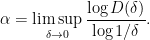
In recent years, it has begun to be realised that in the regime 

(actually in practice we often permit small losses such as 

and taking the square root of both side to conclude that
However, the flip side of this weakness is that (2) can be easier to prove. One key reason for this is the ability to iterate decoupling estimates such as (2), in a way that does not seem to be possible with reverse square function estimates such as (1). For instance, suppose that one has a decoupling inequality such as (2), and furthermore each 
Then by inserting these bounds back into (2) we see that we have the combined decoupling inequality

This iterative feature of decoupling inequalities means that such inequalities work well with the method of induction on scales, that we introduced in the previous set of notes.
In fact, decoupling estimates share many features in common with restriction theorems; in addition to induction on scales, there are several other techniques that first emerged in the restriction theory literature, such as wave packet decompositions, rescaling, and bilinear or multilinear reductions, that turned out to also be well suited to proving decoupling estimates. As with restriction, the curvature or transversality of the different Fourier supports of the
Strikingly, in many important model cases, the optimal decoupling inequalities (except possibly for epsilon losses in the exponents) are now known. These estimates have in turn had a number of important applications, such as establishing certain discrete analogues of the restriction conjecture, or the first proof of the main conjecture for Vinogradov mean value theorems in analytic number theory.
These notes only serve as a brief introduction to decoupling. A systematic exploration of this topic can be found in this recent text of Demeter.
— 1. Square function and reverse square function estimates —
We begin with a form of the Littlewood-Paley inequalities. Given a region 


Theorem 1 (Littlewood-Paley inequalities) Let
, let
be distinct integers, let
let
be a function with Fourier support in the annulus
.
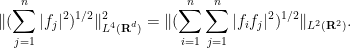
- (i) (Reverse square function inequality) One has
- (ii) (Square function inequality) If the
for any
) then

Proof: We begin with (ii). We use a randomisation argument. Let 


at least for functions 


Now let 

The operator 

uniformly in the 

Now we turn to (i). By treating the

for any

Applying the Hörmander-Mikhlin theorem as before, we conclude that
and on taking

Exercise 2 (Smooth Littlewood-Paley estimate) Let
be a bump function supported on
that equals
on
. For any integer
, let
denote the Fourier multiplier, defined on Schwartz functions
and extended to
functions by continuity. Show that for any
, one has
(in particular, the left-hand side is finite).


We remark that when 
Exercise 3 (Unboundedness of the disc multiplier) Let
denote either the disk
or the annulus
denote the Fourier multiplier defined on Schwartz functions
by
- (i) Show that for any collection
of half-planes in
, and any functions
, that
(Hint: first rescale the set
, apply the Marcinkiewicz-Zygmund theorem (Exercise 7 from Notes 1), exploit the symmetries of the Fourier transform, then take a limit as
.)
- (ii) Let
be a collection of
rectangles for some
, and for each
be a rectangle formed from
by translating by a distance
(Hint: a direct application of (i) will give just one side of this estimate, but then one can use symmetry to obtain the other side.)
- (iii) In Fefferman’s paper, modifying a classic construction of a Besicovitch set, it was shown that for any
, there exists a collection of
rectangles
with
such that all the rectangles
has measure
. Assuming this fact, conclude that the multiplier estimate (4) fails unless
- (iv) Show that Theorem 1(ii) fails when
and the requirement that the


Exercise 4 Let
be a bump function supported on
that equals one on
. For each integer
, let
be the Fourier multiplier defined for
by
and also define
- (i) For any
, establish the square function estimate
for
cases, and for the latter use Plancherel’s theorem for Fourier series.)
- (ii) For any
, establish the square function estimate
for
is bounded in
.)
- (iii) For any
, establish the reverse square function estimate
for
- (iv) Show that the estimate (ii) fails for
, and similarly the estimate (iii) fails for
.

![\displaystyle \widehat{P_{[n,n+1]} f}(\xi) := 1_{[n,n+1]}(\xi) \hat f(\xi).](https://s0.wp.com/latex.php?latex=%5Cdisplaystyle+%5Cwidehat%7BP_%7B%5Bn%2Cn%2B1%5D%7D+f%7D%28%5Cxi%29+%3A%3D+1_%7B%5Bn%2Cn%2B1%5D%7D%28%5Cxi%29+%5Chat+f%28%5Cxi%29.&bg=ffffff&fg=000000&s=0&c=20201002)

![\displaystyle \| (\sum_{n \in {\bf Z}} |P_{[n,n+1]} f|^2)^{1/2} \|_{L^p({\bf R})} \lesssim_p \|f\|_{L^p({\bf R})}](https://s0.wp.com/latex.php?latex=%5Cdisplaystyle+%5C%7C+%28%5Csum_%7Bn+%5Cin+%7B%5Cbf+Z%7D%7D+%7CP_%7B%5Bn%2Cn%2B1%5D%7D+f%7C%5E2%29%5E%7B1%2F2%7D+%5C%7C_%7BL%5Ep%28%7B%5Cbf+R%7D%29%7D+%5Clesssim_p+%5C%7Cf%5C%7C_%7BL%5Ep%28%7B%5Cbf+R%7D%29%7D&bg=ffffff&fg=000000&s=0&c=20201002)
![\displaystyle \|f\|_{L^p({\bf R})} \lesssim_p \| (\sum_{n \in {\bf Z}} |P_{[n,n+1]} f|^2)^{1/2} \|_{L^p({\bf R})}](https://s0.wp.com/latex.php?latex=%5Cdisplaystyle+%5C%7Cf%5C%7C_%7BL%5Ep%28%7B%5Cbf+R%7D%29%7D+%5Clesssim_p+%5C%7C+%28%5Csum_%7Bn+%5Cin+%7B%5Cbf+Z%7D%7D+%7CP_%7B%5Bn%2Cn%2B1%5D%7D+f%7C%5E2%29%5E%7B1%2F2%7D+%5C%7C_%7BL%5Ep%28%7B%5Cbf+R%7D%29%7D&bg=ffffff&fg=000000&s=0&c=20201002)
Remark 5 The inequalities in Exercise 4 have been generalised by replacing the partition
with an arbitrary partition of the real line into intervals; see this paper of Rubio de Francia.
If 
We have the following variants of this claim:
Lemma 6 (
and
reverse square function estimates) Let
respectively.
- (i) (Almost orthogonality) If the sets
have overlap at most
(i.e., every
lies in at most
) for some
, then
- (ii) (Almost bi-orthogonality) If the sets
with
have overlap at most
for some
, then

Proof: For (i), observe from Plancherel’s theorem that

By hypothesis, for each frequency 
and hence by Fubini’s theorem
The claim then follows by a further application of Plancherel’s theorem and Fubini’s theorem. For (ii), we observe that
and
Since 

Remark 7 By using
in place of
. It is also clear how to extend the lemma to other even exponent Lebesgue spaces such as
; see for instance this recent paper of Gressman, Guo, Pierce, Roos, and Yung. However, we will not use these variants here.
We can use this lemma to establish the following
Exercise 8 (Square function estimate for circle and parabola) Let
, let
-separated subset of the unit circle
, and for each
, let
have Fourier support in the rectangle
- (i) Use Lemma 6(ii) to establish the reverse square function estimate
- (ii) If the elements of
-separated for a sufficiently large absolute constant
, establish the matching square function estimate
- (iii) Obtain analogous claims to (i), (ii) in which
for some
-separated subset
of
, where
is the graphing function
, and to each
one uses the parallelogram
in place of
.
- (iv) (Optional, as it was added after this exercise was first assigned as homework) Show that in (i) one cannot replace the
. (Hint: use a Knapp type example for each
and ensure that there is enough constructive interference in
near the origin.) On the other hand, using Exercise 4 show that the


For a more sophisticated estimate along these lines, using sectors of the plane rather than rectangles near the unit circle, see this paper of Cordóba. An analogous reverse square function estimate is also conjectured in higher dimensions (with 
— 2. Decoupling estimates —
We now turn to decoupling estimates. We begin with a general definition.
Definition 9 (Decoupling constant) Let
be a finite collection of non-empty open subsets of
(we permit repetitions, so
may be a multi-set rather than a set), and let
. We define the decoupling constant
to be the smallest constant for which one has the inequality
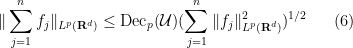
 has Fourier support in
 We have the trivial upper and lower bounds

with the lower bound arising from restricting to the case when all but one of the 


Exercise 10 (Elementary properties of decoupling constants) Let
- (i) (Monotonicity) Show that
whenever
are non-empty open subsets of
for
- (ii) (Triangle inequality) Show that
for any finite non-empty collections
of open non-empty subsets of
- (iii) (Affine invariance) Show that
whenever
are open non-empty and
is an invertible affine transformation.
- (iv) (Interpolation) Suppose that
for some
and
, and suppose also that
for all
,
, and
is defined by
Show that
- (v) (Multiplicativity) Suppose that
is a family of open non-empty subsets of
containing further open non-empty subsets
for
. Show that
- (vi) (Adding dimensions) Suppose that
is a family of disjoint open non-empty subsets of
. Show that for any
, one has
where the right-hand side is a decoupling constant in
.


The most useful decoupling inequalites in practice turn out to be those where the decoupling constant
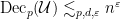
for every
For 

if the sets
when the sets 
For 

Exercise 11 If
for any
. (Hint: select the
Henceforth we now focus on the regime 

Exercise 12 If
, and
(Hint: for the upper bound, use a variant of Exercise 24(ii) from Notes 1, or adapt the interpolation arguemnt used to establish that exercise.)
Now we establish a significantly more non-trivial decoupling theorem:
Theorem 13 (Decoupling for the parabola) Let
, and to each
be the parallelogram (5). Then
for any
This result was first established by Bourgain and Demeter; our arguments here will loosely follow an argument of Li, that is based in turn on the efficient congruencing methods of Wooley, as recounted for instance in this exposition of Pierce.
We first explain the significance of the exponent 


for all
On the other hand, we have 


Comparing this with (6), we conclude that
so Theorem 13 cannot hold if the exponent 


For any 


for any
We first make a minor observation on the stability of 
 are such that
  then
then  .
.Proof: Without loss of generality we may assume that 


whenever 


The claim now follows from Exercise 10(i) and the inclusion

Conversely, we need to show that

whenever ![{\Sigma' \subset [-1,1]}](https://s0.wp.com/latex.php?latex=%7B%5CSigma%27+%5Csubset+%5B-1%2C1%5D%7D&bg=ffffff&fg=000000&s=0&c=20201002)

when 


![{[\xi'-\delta',\xi'+\delta']}](https://s0.wp.com/latex.php?latex=%7B%5B%5Cxi%27-%5Cdelta%27%2C%5Cxi%27%2B%5Cdelta%27%5D%7D&bg=ffffff&fg=000000&s=0&c=20201002)


where each 

Now the collection 

and thus

Applying (10), (11) we obtain the claim.
More importantly, we can use the symmetries of the parabola to control decoupling constants for parallelograms 


Proposition 15 (Parabolic rescaling) Let
, and let
of length
. Then

Proof: We can assume that 


![{I = [\xi_0-\delta_0,\xi_0+\delta_0]}](https://s0.wp.com/latex.php?latex=%7BI+%3D+%5B%5Cxi_0-%5Cdelta_0%2C%5Cxi_0%2B%5Cdelta_0%5D%7D&bg=ffffff&fg=000000&s=0&c=20201002)

(which preserves the parabola, and maps parallelograms 

![{\Sigma \subset [-\delta_0,\delta_0]}](https://s0.wp.com/latex.php?latex=%7B%5CSigma+%5Csubset+%5B-%5Cdelta_0%2C%5Cdelta_0%5D%7D&bg=ffffff&fg=000000&s=0&c=20201002)
Now let 

Observe that 


since 

 for all
  .
.The multiplicativity property in Exercise 16 suggests that an induction on scales approach could be fruitful to establish (9). Interestingly, it does not seem possible to induct directly on
Definition 17 (Bilinear decoupling constant) Let
. Define
to be the best constant for which one has the estimate
whenever
are
of length
respectively with
, and for each
,
has Fourier support in
, and similarly for each
,
has Fourier support in
.


The scale 


From Hölder’s inequality, the left-hand side of (13) is bounded by

from which we conclude the bound

When 

Proposition 18 (Bilinear reduction) If
, then

Proof: Let 

We partition 


From the pigeonhole principle, this implies at least one of the following statements needs to hold for each given 
- (i) (Narrow case) There exists
such that
- (ii) (Broad case) There exist distinct intervals
with
such that


(The reason for this is as follows. Write 


(We remark that more advanced versions of this “narrow-broad decomposition” in higher dimensions, taking into account more of the geometry of the various frequencies 

while from Proposition 15 we have

and hence


Combining all these estimates, we obtain the claim.
In practice the 


If we immediately apply insert (14) into the above lemma, we obtain a useless inequality due to the loss of 
Proposition 19 (Key estimate) If
with
then

Proof: It will suffice to show that

whenever 
![{I, J \subset [-1,1]}](https://s0.wp.com/latex.php?latex=%7BI%2C+J+%5Csubset+%5B-1%2C1%5D%7D&bg=ffffff&fg=000000&s=0&c=20201002)


We can partition 


where

and

From (13) we have

so it will suffice to prove the almost orthogonality estimate

By Lemma 6(i), it suffices to show that the Fourier supports of 

Applying a Galilean transformation, we may normalise the interval 
![{J = [-\rho_2/2,\rho_2/2]}](https://s0.wp.com/latex.php?latex=%7BJ+%3D+%5B-%5Crho_2%2F2%2C%5Crho_2%2F2%5D%7D&bg=ffffff&fg=000000&s=0&c=20201002)


![{[-2,2]}](https://s0.wp.com/latex.php?latex=%7B%5B-2%2C2%5D%7D&bg=ffffff&fg=000000&s=0&c=20201002)


![{\xi \in [-2,2]}](https://s0.wp.com/latex.php?latex=%7B%5Cxi+%5Cin+%5B-2%2C2%5D%7D&bg=ffffff&fg=000000&s=0&c=20201002)


The final ingredient needed is a simple application of Hölder’s inequality to allow one to (partially) swap 

Exercise 20 For any
, establish the inequality

Now we have enough inequalities to establish the claim (9). Let 
for all
Another equivalent formulation is that

as 


Suppose for contradiction that 

as 
Let

Since 


if

for various 


and then by Proposition 19

if

The crucial fact here is that we gain a small power of 


for any given 


which when inserted back into (20), (19) gives

If we then choose
Remark 21 An alternate arrangement of the above argument is as follows. For any exponent
, let
denote the claim that
whenever
fixed. The bounds (14), (17) give the claim
. On the other hand, the bound (21) shows that
for any given

Exercise 22 By carefully unpacking the above iterative arguments, establish a bound of the form
for all sufficiently small
. (This bound was first established by Li.)

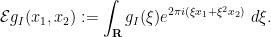
Exercise 23 (Localised decoupling) Let
be an integrable function supported on
denote the extension operator
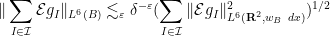
For any ball
of radius
, use Theorem 13 to establish the local decoupling inequality
for any
is the weight function

The decoupling theorem for the parabola has been extended in a number of directions. Bourgain and Demeter obtained the analogous decoupling theorem for the paraboloid:
Theorem 24 (Decoupling for the paraboloid) Let
, let
, where
is the map
, and to each
let
be the disk
Then one has
for any

Clearly Theorem 13 is the
Exercise 25 Show that the exponent
in Theorem 24 cannot be replaced by any larger exponent.
We will not prove Theorem 24 here; the proof in Bourgain-Demeter shares some features in common with the one given above (for instance, it focuses on a 
Somewhat analogously to how the multilinear Kakeya conjecture could be used in Notes 1 to establish the multilinear restriction conjecture (up to some epsilon losses) by an induction on scales argument, the decoupling theorem for the paraboloid can be used to establish decoupling theorems for other surfaces, such as the sphere:
Exercise 26 (Decoupling for the sphere) Let
. To each
be the disk
Assuming Theorem 24, establish the bound
for any
denote the supremum over all expressions of the form of the left-hand side of (23), use Exercise 10 and Theorem 24 to establish a bound of the form
, taking advantage of the fact that a sphere resembles a paraboloid at small scales. This argument can also be found in the above-mentioned paper of Bourgain and Demeter.)


An induction on scales argument (somewhat similar to the one used to establish the multilinear Kakeya estimate in Notes 1) can similarly be used to establish decoupling theorems for the cone

from the decoupling theorem for the parabola (Theorem 13). It will be convenient to rewrite the equation for the cone as 
which can be viewed as a projective version of the parabola 
Exercise 27 (Decoupling for the cone) For
denote the supremum of the decoupling constants
where
denotes the sector
More generally, if
, let
denote the supremum of the decoupling constants
where
denotes the shortened sector
- (i) For any
, show that
.
- (ii) For any
for any
- (iii) For any
, show that
. (Hint: adapt the argument used to establish Exercise 16, taking advantage of the invariance of the tilted light cone under projective parabolic rescaling
and projective Galilean transformations
; these maps can also be viewed as tilted (conformal) Lorentz transformations ).
- (iv) Show that
for any
- (v) State and prove a generalisation of (iv) to higher dimensions, using Theorem 24 in place of Theorem 13.
This argument can also be found in the above-mentioned paper of Bourgain and Demeter.


A separate generalization of Theorem 13, to the moment curve

was obtained by Bourgain, Demeter, and Guth:
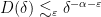
Theorem 28 (Decoupling for the moment curve) Let
, let
denote the region
where
is the map
Then
for any
![\displaystyle R_{t,\delta} := \{ \xi \in {\bf R}^d: |\xi - \phi(t')| \leq \delta^d \hbox{ for some } t' \in [t-\delta,t+\delta] \}](https://s0.wp.com/latex.php?latex=%5Cdisplaystyle+R_%7Bt%2C%5Cdelta%7D+%3A%3D+%5C%7B+%5Cxi+%5Cin+%7B%5Cbf+R%7D%5Ed%3A+%7C%5Cxi+-+%5Cphi%28t%27%29%7C+%5Cleq+%5Cdelta%5Ed+%5Chbox%7B+for+some+%7D+t%27+%5Cin+%5Bt-%5Cdelta%2Ct%2B%5Cdelta%5D+%5C%7D&bg=ffffff&fg=000000&s=0&c=20201002)

Exercise 29 Show that the exponent
in Theorem 28 cannot be replaced by any higher exponent.
It is not difficult to use Exercise 10 to deduce Theorem 13 from the 

The original proof of Theorem 28 by Bourgain-Demeter-Guth was rather intricate, using for instance a version of the multilinear Kakeya estimate from Notes 1. A shorter proof, similar to the one used to prove Theorem 13 in these notes, was recently given by Guo, Li, Yung, and Zorin-Kranich, adapting the “nested efficient congruencing” method of Wooley, which we will not discuss here, save to say that this method can be viewed as a
Perhaps the most striking application of Theorem 28 is the following conjecture of Vinogradov:
Exercise 30 (Main conjecture for the Vinogradov mean value theorem) Let
and any
, let
denote the quantity
where
.
- (i) If
is a natural number, show that
of natural numbers between
obeying the system of equations
for
.
- (ii) Using Theorem 28, establish the bound
for all
. (Hint: set
and
, and apply the decoupling inequality to functions
that are adapted to a small ball around
.)
- (iii) More generally, establish the bound
for any
factors.
![\displaystyle J_{s,d}(N) := \int_{[0,1]^d} |\sum_{n=1}^N e( x_1 n + x_2 n^2 + \dots + x_d n^d )|^{2s}\ dx_1 \dots dx_n](https://s0.wp.com/latex.php?latex=%5Cdisplaystyle+J_%7Bs%2Cd%7D%28N%29+%3A%3D+%5Cint_%7B%5B0%2C1%5D%5Ed%7D+%7C%5Csum_%7Bn%3D1%7D%5EN+e%28+x_1+n+%2B+x_2+n%5E2+%2B+%5Cdots+%2B+x_d+n%5Ed+%29%7C%5E%7B2s%7D%5C+dx_1+%5Cdots+dx_n&bg=ffffff&fg=000000&s=0&c=20201002)


Remark 31 Estimates of the form (24) are known as mean value theorems, and were first established by Vinogradov in 1937 in the case when
for which (24) was established was improved over the years, with much recent progress by Wooley using his method of efficient congruencing; see this survey of Pierce for a detailed history. In particular, these methods can supply an alternate proof of (24); see this paper of Wooley.
Exercise 32 (Discrete restriction) Let
. Using Theorem 24 and Exercise 26, show that for any radius
and any complex numbers
, one has the discrete restriction estimate
Explain why the exponent


For further applications of decoupling estimates, such as restriction and Strichartz estimates on tori, and application to combinatorial incidence geometry, see the text of Demeter.
[These exercises will be moved to a more appropriate location at the end of the course, but are placed here for now so as not to affect numbering of existing exercises.]
Exercise 33 Show that the inequality in (8) is actually an equality, if
is the maximal overlap of the
Exercise 34 Show that
whenever
. (Hint: despite superficial similarity, this is not related to Lemma 14. Instead, adapt the parabolic rescaling argument used to establish Proposition 15.)

95 comments
Comments feed for this article
14 April, 2020 at 3:06 am
mohsen
Hello professor.
A PURPOSE!
Please put your pdf version of your notes on this website too!
thanks alot!
14 April, 2020 at 4:07 am
Anonymous
This has been asked many times. See for instance this thread: https://terrytao.wordpress.com/2020/03/29/247b-notes-1-restriction-theory/#comment-549677
If you print a blog post to PDF it should be fairly readable.
14 April, 2020 at 4:31 am
Irkutsk
There should be an absolute value on the LHS of the first displayed formula.
14 April, 2020 at 5:29 am
shapiro
In Exercise 4 (iv), what kind of counterexamples should I be looking at? I tried a family of dilated bump functions but it is really tough to compute the projections on frequency. I do not even know if this is the right family of function to test. Do you have any hint?
14 April, 2020 at 6:08 am
shapiro
Well, it seems that after writing this comment I finally found an answer: condering a function f such that P_[k,k+1] (f)= the same bump function works just fine!
14 April, 2020 at 5:48 am
Trevor Wooley
Just a note on nomenclature: in Exercise 30 you refer to the “Vinogradov main conjecture”, which seems to have entered usage in the literature in the past few years in the harmonic analysis community. In the number theory community the name has been different, partly owing to the fact that there are many conjectures associated with the name I. M. Vinogradov, including for example his famous conjecture concerning non-trivial cancellation in short character sums. The phrase “Vinogradov’s mean value theorem” was used to describe any non-trivial estimate (optimal or not) for the mean value of exponential sums (or moment estimate) in question, and the estimate in Exercise 30 was often referred to as the “optimal estimate in Vinogradov’s mean value theorem”, or by me and others over the past decade as the “main conjecture in Vinogradov’s mean value theorem”.
For what it is worth, the “nested efficient congruencing method” can be seen as a p-adic decoupling method, which leads to some unification of all the ideas currently in play.
14 April, 2020 at 7:57 am
Terence Tao
Thanks for this! I realise that I have indeed mentally contracted “main conjecture for the Vinogradov mean value theorem” as “Vinogradov main conjecture”, and have now corrected this in the text. Also I realise that in my rush to push out these notes I had omitted the historical remarks on this conjecture, which I have now also added.
27 April, 2020 at 9:14 pm
Anon
Could you describe what a p-adic decoupling method is (even if the term isn’t strictly defined)?
3 May, 2020 at 5:50 pm
Anon
Dear Professor Tao, you are also welcome to answer this if you wish.
14 April, 2020 at 6:28 am
Lior Silberman
In the line after equation (1), it is the that are supported on the annuli, right? (I guess you follow the physics convention where the variable name specifies the coordinate system).
[Corrected, thanks – T.]
14 April, 2020 at 6:36 am
Lior Silberman
In the equation after you mention Hormander–Miklin there is a missing on the LHS and the subscript didn’t come out.
[Corrected, thanks – T.]
14 April, 2020 at 5:33 pm
Anon
Note:the same small issue also appears at end of proof of Thm1
[Corrected, thanks – T.]
14 April, 2020 at 6:38 am
Lior Silberman
In exercise 2 you need to swap the two balls (so the bump function is supported on the ball of radius 2, equal to 1 on the ball of radius 1).
[Corrected, thanks – T.]
14 April, 2020 at 11:24 am
extremal010101
proof of theorem 1, part (i): why ? I assume
  . The bump function
  is supported on
  , and the frequencies of
  are not “2-separated”, then
  may have frequencies not in
  , or am I missing something?
14 April, 2020 at 11:47 am
Terence Tao
In this part of the argument we are proving (ii), not (i).
17 April, 2020 at 5:16 am
dn1214
In Exercise 4 (i), how do you use Parseval for series to get the case? If I introduce the function
  then I can not compute easily the
  norm of this function and I’m stuck.
The proof I know goes roughly as follows: for any we write
  where
where  and then we use the decay of
  to conclude.
17 April, 2020 at 10:20 am
Terence Tao
The function can be expressed in terms of
  in a tractable form using either the Poisson summation formula or the Fourier inversion formula for periodic functions, after a certain amount of standard manipulation using the usual Fourier identities. The duality method you indicate would also work.
27 April, 2020 at 12:01 pm
hhy177
To apply the Poisson summation formula here, don’t we need to be Schwartz in
  ? Writing
  , it seems like
  is smooth with not enough decay in
  . After I proceed formally with this calculation (such as taking inverse Fourier transform of 1 in the process), I seem to get something looking more tractable, from which I could derive the boundedness of the square estimate in 4.(i) when
  .
.
27 April, 2020 at 12:44 pm
Terence Tao
To convert your formal computations to a rigorous argument, one can either (a) try to work in the language of (tempered) distributions, (b) using some sort of limiting argument, or (c) take the final expression for that you obtained and try to prove it by a different (and fully rigorous) method (e.g., by first establishing a “Fourier transform” of your identity and then applying the Fourier inversion formula).
19 April, 2020 at 5:42 am
dn1214
I have two questions about exercise 3: and
and  are two fully independent collections of rectangles (pick one collection of disjoint rectangles, and the other to be all the same rectangle), I am wondering how to use that the
  are translations of
  ? Does it require to use the boundedness of the disc multiplier?
 ), is it normal?
– In (ii) I am not able to prove the result; since the result is false if
– I was surprised that without using (ii), one can solve (iv) only using (i) (taking
There is also a minor typo: at the begining of the exercise, I guess.
Thank you a lot.
19 April, 2020 at 11:56 am
Terence Tao
Yes, one should use part (i) to establish part (ii).
The definition of encompasses both
  and
and  , which is why I used a different symbol from either here.
21 April, 2020 at 10:22 am
dn1214
Thank you for the clarification!
21 April, 2020 at 12:02 am
Anonymous
I’m curious if one should expect to be able to replace the ball of integration on the left in the local decoupling estimates with an integral over a smaller more tubular region?
It seems that when you ultimately rescale and plug in lattice points to prove Vinogrodov-type estimates, there ends up being redundancy in the integral, and that an estimate over a more tubular region would more naturally lead to a the the exact Vinogrodov integral (and be a stronger estimate).
21 April, 2020 at 7:30 am
Terence Tao
Good question. There are counterexamples that show that the balls on which decoupling occurs cannot be replaced by smaller balls without significant increase in the decoupling constants, but there may be some possibility of additional useful decoupling estimates involving more eccentric domains than balls. For instance if one is trying to decouple arcs in Fourier space contained in a narrow arc of the paraboloid, then by applying a suitable Galilean transformation and parabolic rescaling, followed by Exercise 23, one obtains a local decoupling estimate involving a certain rectangular region that is a little bit smaller in one dimension than the ball one would get from direct application of Exercise 23. So perhaps there is some “time-frequency” version of decoupling that is a little bit smarter about the spatial localisation, and as you say the redundancy in the Vinogradov integral also points to some possibility of improvement in this direction also.
21 April, 2020 at 10:47 pm
dn1214
Aren’t there typos in the proof of Lemma 14? e.g. “assuming that “, since we have
  , I would expect a
  sign. And in the proof you write “since
  contains
  “: one of the
  should be a
  .
.
22 April, 2020 at 7:57 am
Terence Tao
The additional restriction is intentional; if one can prove the claim in the special case
  then by transitivity one then obtains the general case
  as a corollary, because in the latter case one can find a third scale
  for which
  .
.
The statement “ contains
  ” is stated correctly, but there is an unfortunate placement of a comma immediately afterwards.
27 April, 2020 at 1:02 am
Rex
It might be helpful to add a white space just before the comma, so that it doesn’t get confused with a prime. I was also disoriented for a moment by this.
[Reworded -T.]
24 April, 2020 at 1:48 pm
Anonymous
In the proof of Theorem 1, how does one get that ?
?
24 April, 2020 at 2:53 pm
Anonymous
Multiplier equals 1 on the fourier support of f_j and 0 for all the others
24 April, 2020 at 3:24 pm
Terence Tao
By computing Fourier transforms one can see that is equal to
  when
when  and vanishes when
  .
.
24 April, 2020 at 1:54 pm
Anonymous
Can one say that “decoupling” is sort of “partition of unity” in the Fourier space? (I may have a very wrong impression.)
24 April, 2020 at 3:27 pm
Terence Tao
Decoupling is a property of some partitions of unity in Fourier space, but not all partitions of Fourier space have good decoupling estimates (and some partitions only have good decoupling for some exponents and not others). The presence of an
  decoupling estimate can be viewed as saying that the
  geometry of that partition behaves somewhat like a Hilbert space geometry in the sense that a (weak) version of the Pythagorean theorem remains valid in this setting.
24 April, 2020 at 5:24 pm
Anonymous
In high dimension, if we use a dyadic cubic projection rather than the dyadic ball projection in the note, can the condition that the
  being 2-separated be removed from Theorem 1(ii)? This would at least avoid encountering the disk multiplier.
[Yes – T.]
25 April, 2020 at 3:08 am
Rex
In exercise 10.ii (triangle inequality), one of the mathcal Us in the statement of the inequality is missing a ‘
[Corrected, thanks – T.]
25 April, 2020 at 6:47 pm
Rex
Does this blog entry load correctly for the other people? I am getting something very messy with “formula does not parse”, visible “”, “”, etc. everywhere starting about 10 hours ago. Everything was fine before then. No other blog entries seem to have this issue.
[Corrected, thanks – T.]
25 April, 2020 at 7:56 pm
Rex
Minor omission: in the proof of lemma 6, the A in “By hypothesis, for each frequency {\xi} at most {A} of the {\hat f_j(\xi)} are non-zero, thus by Cauchy-Schwarz” is missing a subscript.
26 April, 2020 at 5:05 am
Xiao-Chuan Liu
For Exercise 3, I can compute and obtain that will take uniform positive value restricted to
  . Is there some easy way to see this should be true (without computing it)?
26 April, 2020 at 8:44 am
Terence Tao
Not really: lower bounds generally are more delicate than upper bounds and usually require some calculation to ensure that one does not have some unexpected cancellation. (In some cases, the function will obey some sort of PDE and one can use tools from the theory of unique continuation to obtain some lower bounds. It’s possible that one could pull off this trick here using the connection between the Hilbert transform and harmonic conjugates, but it is simpler to just directly calculate in this case.)
26 April, 2020 at 6:36 am
Rex
The formula
“ .”
.”
under Theorem 13 has a \Vert on the left and a parenthesis on the right.
[Corrected, thanks – T.]
27 April, 2020 at 12:04 pm
hhy177
For Ex 4 (ii), how do one see the boundedness of![P_{[0,1]}](https://s0.wp.com/latex.php?latex=P_%7B%5B0%2C1%5D%7D&bg=ffffff&fg=545454&s=0&c=20201002) on
on  from the boundedness of the Hilbert transform? Since both operator is equal (up to a factor of
  ) on Schwartz functions with Fourier support in
 ![[0,1]](https://s0.wp.com/latex.php?latex=%5B0%2C1%5D&bg=ffffff&fg=545454&s=0&c=20201002) , I can conclude
, I can conclude ![P_{[0,1]}](https://s0.wp.com/latex.php?latex=P_%7B%5B0%2C1%5D%7D&bg=ffffff&fg=545454&s=0&c=20201002) is bounded on on Schwartz functions with Fourier support in
is bounded on on Schwartz functions with Fourier support in ![[0,1]](https://s0.wp.com/latex.php?latex=%5B0%2C1%5D&bg=ffffff&fg=545454&s=0&c=20201002) . How do I see it for arbitrary functions?
. How do I see it for arbitrary functions?
27 April, 2020 at 12:45 pm
Terence Tao
Express![P_{[0,1]}](https://s0.wp.com/latex.php?latex=P_%7B%5B0%2C1%5D%7D&bg=ffffff&fg=545454&s=0&c=20201002) as the difference of
as the difference of  and
and  .
.
27 April, 2020 at 9:46 pm
Anonymous
Dear Pro Tao,
Whether you want it or not, Twin prime conjecture is certainly solved in 2020. By any rate, you must succeed. The historic seconds is coming, you have no choice. An only way for you, you can not come back, only go aheah! I think Sir will understand my imply. As you win , it will be useful for many people.
Lovely Pro.Tao,
28 April, 2020 at 9:35 am
Anonymous
What’s this about?
27 April, 2020 at 1:56 pm
Anonymous
Dear Professor Tao, in the proof of the Key estimate (Proposition 19), you said “ , hence
  “. I think one needs
  in order to do so. Otherwise, could you please give me some hints on how it works? Thank you very much.
[Oops, there are some losses of here that I forgot to take into account; however, these turn out to be acceptable losses for this argument, which is now reworded accordingly. -T]
28 April, 2020 at 12:02 pm
Rex
In the proof of lemma 14:
“(we can extend from {C^\infty_c({\bf R}^2)} to all of {L^6({\bf R}^2)} by a limiting argument).”
I assume that this should be changed to Schwartz functions?
[Corrected, thanks – T.]
29 April, 2020 at 11:41 am
Anonymous
For the triangle inequality of decoupling constants, I got the inequality the other way around. I basically used the monotonicity for U and U’ (i.e. ), square both sides then add them, and take square root, I got

How to get the inequality the other way around?
29 April, 2020 at 2:24 pm
Lior Silberman
Apply the 2d C–S inequality to the dot product where
where  (resp.
  ) have Fourier support in
  (resp.
  ).
).
29 April, 2020 at 2:56 pm
Terence Tao
One trick that can help conceptually with trying to prove estimates of the form or
or  is to deconstruct the degenerate version of these inequalities, namely that “If
  vanishes (or is very small), then
  must also vanish (or is very small)”. Suppose you know that
  vanishes (or is very small). What does this tell you about
  ? If one approaches this question literally it is vacuous due to the fact that decoupling constants are necessarily bounded from below by 1, but try to ignore this fact for the purposes of performing a mental exercise. Your answer to this exercise will help suggest how to actually approach the inequality at hand.
29 April, 2020 at 2:26 pm
Lior Silberman
Question about Ex. 10(v): where do we use the disjointness? It seems to me that the argument works whenever are any sets such that (up to sets of measure zero)
  .
.
[Good point; I’ve reworded the exercise accordingly. -T]
29 April, 2020 at 3:19 pm
Anonymous
In the explanation of significance of , how do you get the factor of
  for the
  norm of
  , ie.
, ie.
 (the 2nd equation after Theorem 13)? Also, I am not sure how do you get
  in the 3rd equation after we restrict
  to a small ball of radius
  .
.
29 April, 2020 at 6:26 pm
Terence Tao
Both of these follow from the previously mentioned fact that has cardinality
  .
.
1 May, 2020 at 6:49 am
Rex
In proof of Prop 18:
“(ii) (Broad case) There exist distinct intervals {I,J \in {\mathcal I}} with {\mathrm{dist}(I,J) \geq \nu} such that
\displaystyle |\sum_{\omega \in \phi(\Sigma)} f_\omega(x)| \lesssim \nu^{-O(1)} |\sum_{\omega \in \phi(\Sigma_I)} f_\omega(x)|, \nu^{-O(1)} |\sum_{\omega \in \phi(\Sigma_I)} f_\omega(x)|.”
One of the subscripts should be a _J instead of a _I, I assume.
Could you say more about how this pigeonhole argument works? I’m not seeing why the broad case should follow if the narrow case doesn’t hold.
[More details added – T.]
1 May, 2020 at 8:48 am
Rex
More in the same proof:
“From (13) we have
\displaystyle \int_{{\bf R}^2} |\sum_{\omega \in \phi(\Sigma_I)} f_\omega|^2 |\sum_{\omega \in \phi(\Sigma_I)} f_\omega|^4 \lesssim M_{2,4}(\delta,\nu,\nu,\nu)
while”
Another subscript here should be _J, and the constant M should be M^6
[Corrected, thanks – T.]
1 May, 2020 at 11:27 am
Rex
In the same proof:
“If we immediately apply insert (14) into the above lemma, we obtain a useless inequality due to the loss of {\nu^{-O(1)})} in the main term on the…”
has an extra parenthesis.
[Corrected, thanks – T.]
1 May, 2020 at 7:51 am
Anonymous
Is the subset really supposed to be a subset of
 ![[\xi' - 10\delta, \xi' + 10\delta]](https://s0.wp.com/latex.php?latex=%5B%5Cxi%27+-+10%5Cdelta%2C+%5Cxi%27+%2B+10%5Cdelta%5D&bg=ffffff&fg=545454&s=0&c=20201002) and of cardinality O(1)? Shouldn’t it be
and of cardinality O(1)? Shouldn’t it be ![[\xi' - \delta', \xi' + \delta']](https://s0.wp.com/latex.php?latex=%5B%5Cxi%27+-+%5Cdelta%27%2C+%5Cxi%27+%2B+%5Cdelta%27%5D&bg=ffffff&fg=545454&s=0&c=20201002) and the cardinality isn’t used in the rest of the proof.
and the cardinality isn’t used in the rest of the proof.
[Corrected, thanks. The cardinality bound is needed for a minor reason, namely to ensure that the polygons formed by taking various boolean combinations of the parallelograms involved only have sides. -T.]
1 May, 2020 at 11:04 am
Anonymous
Should the RHS of eq.(13) in the definition of bilinear decoupling constant be instead of
  ?
?
1 May, 2020 at 11:11 am
Anonymous
Sorry, it is right.
1 May, 2020 at 12:24 pm
Alan Chang
In the proof of Lemma 14, why do you assume instead of just
  ?
?
2 May, 2020 at 8:32 am
Terence Tao
Huh, I think that was a relic from an earlier version of the argument. You are right, the extra safety margin of is not needed here.
1 May, 2020 at 2:41 pm
Lior Silberman
In the second equation after (21), I would replace with
with  .
.
[Corrected, thanks – T.]
3 May, 2020 at 1:37 am
Rex
In the proof of Prop 19:
“we have the normalisation
\displaystyle \sum_{\omega_1 \in \phi(\Sigma_1)} \|f_{\omega_1}\|_{L^6({\bf R}^2)} = \sum_{\omega_2 \in \phi(\Sigma_2)} \|g_{\omega_2}\|_{L^6({\bf R}^2)}^2 = 1.
We can partition {\Sigma_1} as {\sum_{I’ \in {\mathcal I}’} \Sigma_{1,I’}}, where {{\mathcal I}’} is a collection of intervals”
The left side of the displayed formula is missing an exponent of 2 (sum of squares of norms rather than norms).
[Corrected, thanks – T.]
3 May, 2020 at 12:01 pm
Rex
In the same proof:
“We can partition {\Sigma_1} as {\sum_{I’ \in {\mathcal I}’} \Sigma_{1,I’}}, where {{\mathcal I}’} is a collection of intervals {I’ \subset [-1,1]} of length {\rho’_1} that have bounded overlap,”
I think here you mean to write union rather than sum over the I’.
[Corrected, thanks – T.]
3 May, 2020 at 12:04 pm
Rex
(or better yet, \coprod since this is a disjoint union)
3 May, 2020 at 12:26 pm
Rex
Also
“here
\displaystyle F_{I’} := \sum_{\omega_1 \in \phi(\Sigma_{1,I})} f_{\omega_1}
and”
has a missing ‘ in the subscript
[Corrected, thanks – T.]
3 May, 2020 at 7:59 am
Alan Chang
In the Knapp-type example to show that decoupling cannot hold for , is there a good way to understand why Khintchine cannot be used to obtain a good lower bound for
  ?
?
In the notes, we used the following pointwise bound: on a ball of radius
However, by randomization, we could instead try to use the following pointwise bound: on a ball of radius
  .
.
To me, it is not clear at first which of these two estimates will do better. After some computations, I see that the random estimate doesn’t give anything useful about (since all the
  s cancel out), but is there a way to see this in advance?
3 May, 2020 at 8:34 am
Terence Tao
Khintchine tells us that random sums always decouple on the average (for ):
):
So if one wants to create a good counterexample to decoupling one has to produce constructive interference (in which is significantly larger in magnitude than the square function
  on some non-empty region of space) rather than random-type interference.
3 May, 2020 at 2:18 pm
John Mangual
What is an example of “independent” phases ?
  is a complex number. The relation
  could possibly be replaced with
  or
or  …
…
Also is there any way to visualize Fourier series with disjoint annuli? In position space or momentum space.
3 May, 2020 at 5:45 pm
Alan Chang
In the centered equation preceding (21), should be
be  ?
?
[Corrected, thanks – T.]
4 May, 2020 at 8:05 am
Alan Chang
Actually, now I think that in the displayed equation preceding (21), the should be
  and that this change should propogate down through the displayed equations that follow.
Also, two displayed equations after (21), should be
  .
.
[Corrected, thanks – T.]
4 May, 2020 at 10:40 am
Anonymous
To prove Prop.18, why is it sufficient to prove equation (14)?
5 May, 2020 at 9:48 am
Terence Tao
I assume you mean (15) instead of (14). From (15) and the definition of we conclude that
(noting that in the definition of decoupling constants we are free to normalise without loss of generality), which then gives Proposition 18.
4 May, 2020 at 1:19 pm
Lior Silberman
In the counter-example after the statement of Thm 13 (significance of the exponent 6) shouldn’t be
be  ?
?
[Corrected, thanks – T.]
5 May, 2020 at 11:29 am
Anonymous
What is Exercise 27(ii) supposed to say? I think it’s incomplete as stated. There’s also a typo in the third line after Exercise 20 “for all 00”.
[Corrected, thanks – T.]
5 May, 2020 at 5:50 pm
Alan Chang
In the centered equation above “so it will suffice to prove the almost orthogonality estimate,” the M_{2,4} constant should be raised to the 6th power.
Also, in the last paragraph of that proof, “(with slightly different implied constants in the O() notation” is missing a closing parenthesis.
[Corrected, thanks – T.]
6 May, 2020 at 11:13 am
Garo
What are some of the heuristic explanations for the gap between the best possible decoupling results for curves with torsion and the conjectured bounds on exponential sums? For example, we get decoupling on
  for
for  but expect the estimate to hold for exponential sums up to
  .
.
7 May, 2020 at 10:08 am
Anon
One direct explanation is the lack of self-similarity in the phase, or the lack of a ‘Galilean’ invariance symmetry. For the parabola notice that an affine change of variables of the form preserves the parabola extension operator after a simple change of variables; this is no longer true if the phase is changed to
  . This self-similarity plays an important role in the proof of decoupling inequalities via parabolic rescaling.
8 May, 2020 at 7:37 am
Anonymous
I think an easier way to do the upper bound in Exercise 12 is to interpolate the p = 2 bound from Plancherel with the trivial bound.
[Hint reworded – T.]
9 May, 2020 at 8:40 am
Alan Chang
In the proof of Proposition 19, I see four instances of L^2(R^d) which should be L^2(R^2).
[Corrected, thanks – T.]
2 June, 2020 at 12:37 am
MATH 247B: Modern Real-Variable Harmonic Analysis – Countable Infinity
[…] Decoupling Estimates […]
4 June, 2020 at 2:34 pm
Anonymous
A small comment (please don’t take my words for granted):
For the Littlewood-Paley inequalities, once
is shown, it follows (by choosing optimizing values for ) that the minimum and maximum (over all sign choices) of the expression
are comparable, and therefore we in fact have
After that, Khintchine will yield both directions of the proof.
This may help clarify the second bit of the proof; it is the same idea expressed differently, i.e. one may also prove
and then use Khintchine on either side.
7 June, 2020 at 2:26 pm
Alan Chang
I have two questions about Remark 21.
1. “On the other hand, the bound (21) shows that implies
  for any given
  .”
.”
In the sentence quoted above, should be
be  ?
?
2. “Thus if , we can establish
  for arbitrarily large
  , and for
  large enough we can insert the bound (22) (with {a=1}) into (19), (20) to obtain the required claim (18).”
From (22) with a = 1, we gain a factor , but this is not necessarily an improvement, since the constant in the exponent can depend on theta. It seems like we need the
  to actually be
  ?
?
8 June, 2020 at 8:39 am
Terence Tao
Oops, it isn’t enough to take , one has to take
  sufficiently large depending on
  in order to overcome both the
  losses, and the
  losses when one converts the estimate back to control on
  .
.
Thanks for the corrections!
8 June, 2020 at 9:26 am
Alan Chang
Thanks!
What do you mean by “convert the estimate back to control on “? If we don’t take
  in (22), how do we use (19) and (20)?
8 June, 2020 at 12:06 pm
Terence Tao
There is an easy triangle inequality argument that shows that . Granted, this makes this version of the argument slightly different from the one in the notes, which required more precise bookkeeping of what in this formulation is the
  error, but it hopefully illustrates that that bookkeeping is not an essential part of the argument.
29 September, 2020 at 6:45 pm
zorich
Dear Tao ,
I have a small question, you said:
“Note from the boundedness of the Hilbert transform that a Fourier projection to any polygon of bounded many sides will be bounded in ."
."
But I think polygons can be used to construct the same counter-example as balls.
Use the same construction in Fefferman's example, if (U is the polygon) is bounded in
  ,then for any dilation and rigid motion L
  is also bounded with the same norm.Then rescale U based on a point on its edges (but not vertices) to exhaust the whole half plane.By Fatou's lemma, it implies the boundness of projection to half plane…
1 October, 2020 at 7:51 am
Terence Tao
The square function over any bounded number of half-planes is still bounded. Only the square function over an unbounded number of half-planes becomes unbounded. Similarly, the multiplier to a polygon with boundedly many sides remains bounded in , but as the number of sides goes to infinity, the
  operator norm will also go to infinity (assuming the orientations of the sides are suitably well distributed in space).
4 October, 2020 at 5:06 am
zorich
Thanks a lot! For polygons, to get half plane pointing different directions, we must use rotations, but can’t be controlled by
  If
If  is different rotations.but for spheres, we only need to use translation(multiplied by a phase) and dilation
4 February, 2021 at 8:05 am
Small typo
Small typo on the index of the random signs:
“…with symbol {\sum_{j=1}^n \epsilon_n \psi(\xi/2^{k_j})}.”, should be “…with symbol {\sum_{j=1}^n \epsilon_j\psi(\xi/2^{k_j})}.”
[Corrected, thanks – T.]
26 July, 2021 at 2:24 pm
B
I’m a little confused as to how to make use of the boundedness of the Fourier projection operators in Exercise 10(iv); any advice? I’m guessing it must be needed to get some sort of “reverse interpolation inequality”, but I’m not sure how to make this precise.
[In order to apply an interpolation theorem, such as Riesz-Thorin, the estimates one is interpolating must be allowed to range freely the entirety of an space; one cannot automatically impose a restriction on these functions, such as a requirement that the functions have specified Fourier support, and still expect to have an interpolation theorem. However, one can get around this for this particular problem by inserting Fourier projections into the decoupling inequality to be proven, which permit the functions involved to now have arbitrary Fourier support. -T]
16 September, 2021 at 8:57 am
Anonymous
In the statememt of Ex 3, $\Omega$ should be $D$ right? Or am I missing smth?
[I am defining the projections here for arbitrary sets
  , such as the half-planes
  in part (i). -T.]