
This is a spinoff from the previous post. In that post, we remarked that whenever one receives a new piece of information 


 is the likelihood of this information under the alternative hypothesis , and
  is the likelihood of this information under the null hypothesis . If there are no other hypotheses under consideration, then the two posterior probabilities
  ,
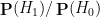
,  must add up to one, and so can be recovered from the posterior odds
  by the formulae

A PDF version of the worksheet and instructions can be found here. One can fill in this worksheet in the following order:
- In Box 1, one enters in the precise statement of the null hypothesis
- In Box 2, one enters in the precise statement of the alternative hypothesis
- In Box 3, one enters in the prior probability
(or the best estimate thereof) of the null hypothesis
- In Box 4, one enters in the prior probability
(or the best estimate thereof) of the alternative hypothesis
.
- In Box 5, one enters in the ratio
between Box 4 and Box 3.
- In Box 6, one enters in the precise new information
- In Box 7, one enters in the likelihood
- In Box 8, one enters in the likelihood
- In Box 9, one enters in the ratio
betwen Box 8 and Box 7.
- In Box 10, one enters in the product of Box 5 and Box 9.
- (Assuming there are no other hypotheses than
divided by
- (Assuming there are no other hypotheses than
To illustrate this procedure, let us consider a standard Bayesian update problem. Suppose that a given point in time, 


We can fill out the entries in the worksheet one at a time:
- Box 1: The null hypothesis
- Box 2: The alternative hypothesis
- Box 3: In the absence of any better information, the prior probability
, or
.
- Box 4: Similarly, the prior probability
.
- Box 5: The prior odds
.
- Box 6: The new information
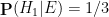
- Box 7: The likelihood
(the false positive rate).
- Box 8: The likelihood
, or
(one minus the false negative rate).
- Box 9: The likelihood ratio
.
- Box 10: The product of Box 5 and Box 9 is approximately
.
- Box 11: The posterior probability
is approximately
.
- Box 12: The posterior probability
is approximately
.
The filled worksheet looks like this:

Perhaps surprisingly, despite the positive COVID test, the employee 
We remark that if we switch the roles of the null hypothesis and alternative hypothesis, then some of the odds in the worksheet change, but the ultimate conclusions remain unchanged:

So the question of which hypothesis to designate as the null hypothesis and which one to designate as the alternative hypothesis is largely a matter of convention.
Now let us take a superficially similar situation in which a mother observers her daughter exhibiting COVID-like symptoms, to the point where she estimates the probability of her daughter having COVID at 
One can fill out the worksheet much as before, but now with the prior probability of the alternative hypothesis raised from 

Thus we see that prior probabilities can make a significant impact on the posterior probabilities.
Now we use the worksheet to analyze an infamous probability puzzle, the Monty Hall problem. Let us use the formulation given in that Wikipedia page:
Problem 1 Suppose you’re on a game show, and you’re given the choice of three doors: Behind one door is a car; behind the others, goats. You pick a door, say No. 1, and the host, who knows what’s behind the doors, opens another door, say No. 3, which has a goat. He then says to you, “Do you want to pick door No. 2?” Is it to your advantage to switch your choice?
For this problem, the precise formulation of the null hypothesis and the alternative hypothesis become rather important. Suppose we take the following two hypotheses:
- Null hypothesis
- Alternative hypothesis
 and
and  . The new information is that, after door 1 is selected, door 3 is revealed and shown to be a goat. After some thought, we conclude that is equal to
  (the host has a fifty-fifty chance of revealing door 3 instead of door 2) but that is also equal to (if the car is behind door 2, the host must reveal door 3, whereas if the car is behind door 3, the host cannot reveal door 3). Filling in the worksheet, we see that the new information does not in fact alter the odds, and the probability that the car is not behind door 1 remains at 2/3, so it is advantageous to switch.

However, consider the following different set of hypotheses:
- Null hypothesis
: The car is behind door number 1, and if you pick the door with the car, the host will reveal another door to entice you to switch. Otherwise, the host will not reveal a door.
- Alternative hypothesis
: The car is behind door number 2 or 3, and if you pick the door with the car, the host will reveal another door to entice you to switch. Otherwise, the host will not reveal a door.
Here we still have 


Finally, we consider another famous probability puzzle, the Sleeping Beauty problem. Again we quote the problem as formulated on the Wikipedia page:
Problem 2 Sleeping Beauty volunteers to undergo the following experiment and is told all of the following details: On Sunday she will be put to sleep. Once or twice, during the experiment, Sleeping Beauty will be awakened, interviewed, and put back to sleep with an amnesia-inducing drug that makes her forget that awakening. A fair coin will be tossed to determine which experimental procedure to undertake:Any time Sleeping Beauty is awakened and interviewed she will not be able to tell which day it is or whether she has been awakened before. During the interview Sleeping Beauty is asked: “What is your credence now for the proposition that the coin landed heads?”‘
- If the coin comes up heads, Sleeping Beauty will be awakened and interviewed on Monday only.
- If the coin comes up tails, she will be awakened and interviewed on Monday and Tuesday.
- In either case, she will be awakened on Wednesday without interview and the experiment ends.
Here the situation can be confusing because there are key portions of this experiment in which the observer is unconscious, but nevertheless Bayesian probability continues to operate regardless of whether the observer is conscious. To make this issue more precise, let us assume that the awakenings mentioned in the problem always occur at 8am, so in particular at 7am, Sleeping beauty will always be unconscious.
Here, the null and alternative hypotheses are easy to state precisely:
- Null hypothesis
- Alternative hypothesis
The subtle thing here is to work out what the correct prior state is (in most other applications of Bayesian probability, this state is obvious from the problem). It turns out that the most reasonable choice of prior state is “unconscious at 7am, on either Monday or Tuesday, with an equal chance of each”. (Note that whatever the outcome of the coin flip is, Sleeping Beauty will be unconscious at 7am Monday and unconscious again at 7am Tuesday, so it makes sense to give each of these two states an equal probability.) The new information is then
- New information
With this formulation, we see that 


There are arguments advanced in the literature to adopt the position that
If one has multiple pieces of information 
 is withheld from the person filling out the worksheet, for instance if that person relies exclusively on a news source that only reports information that supports the alternative hypothesis and omits information that debunks it, then the outcome of the worksheet is likely to be highly inaccurate, and one should only perform a Bayesian analysis when one has a high confidence that all relevant information (both favorable and unfavorable to the alternative hypothesis) is being reported to the user.

28 comments
Comments feed for this article
7 October, 2022 at 4:01 pm
A Bayesian probability worksheet – Marxist Statistics
[…] A Bayesian probability worksheet […]
7 October, 2022 at 6:49 pm
mgflax
Starting in elementary school, we teach children to think of likelihood in terms of a probability lying in [0,1] — and then later Bayesists tell them to exclude 0 and 1 as not actually possible. But I’m wondering if it wouldn’t be more natural to have students *start* with an odds formulation of likelihood, with values lying in (0,\infty). If it’s the natural way gamblers think, perhaps it’s more fundamental in general?
10 October, 2022 at 9:58 am
Terence Tao
In this specific problem of updating Bayesian priors, the prior odds and the posterior odds
 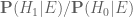 are indeed convenient quantities to use. However for the likelihoods
  ,
,  it is still convenient to use the actual probabilities rather than their associated odds
  ,
,  . Furthermore, many of the laws of probability are easier to state using probabilities than odds. For instance, the union bound
* If ,
,  are two events, then
  is at most
  , with equality when
  are disjoint
or the independence rule
* If ,
,  are two independent events, then
become more unwieldy when phrased in terms of odds. So I think one has to teach both probabilities and odds, and how to convert between each other (much like how one teaches real arithmetic with both decimals and fractions simultaneously); there isn’t a “one-size-fits-all” convention that simplifies all calculations simultaneously.
8 October, 2022 at 10:55 am
Anonymous
In the wikipedia article on the Monty Hall problem (problem 1 above) it is stated that even Erdos had difficulty to accept the correct solution.
8 October, 2022 at 11:59 pm
James Smith
Good to see you linking to the Monty Hall problem on Wikipedia. I remember trying to explain the result to my student a few years back. I had several stabs at it but in the end had to admit to myself, and to my student, that I really didn’t know what I was talking about! The proof that was there didn’t help, it was clearly bogus, so in the end we decided that we should just figure it out from first principles ourselves. Since neither of us were experts, it took several hours!
Here is link to that proof:
https://en.wikipedia.org/w/index.php?title=Monty_Hall_problem&oldid=818327855#Direct_calculation
I give it here because it has since been rewritten again and the current rewrite is perhaps a little less expansive. For this reason, I keep the above link on my home page. Anyway, perhaps the proof will help someone gain some insight.
I still cannot quite believe the end result myself.
9 October, 2022 at 8:48 pm
Des Smith
Please help!
Consider the first example, where 2\% of the population is infected with COVID-19, the COVID-19 test has a 20\% chance of a false negative, and a 5\% chance of a false positive. My na\”ive calculation is that a positive test implies a probability of the test subject actually having the disease of
Using the concrete numbers provided:
This result is somewhat different from the worked example value and, further, does not require the false negative rate which the worked example employs.
What am I doing wrong?
10 October, 2022 at 9:51 am
Terence Tao
The true positive rate is , not
, not  .
.
10 October, 2022 at 10:13 am
Des Smith
Oh yes, I see now, thank you so much. Your comment prompted me to draw out a forking diagram of possibilities and I now understand much better. Thanks so much again!
12 October, 2022 at 6:30 am
Vincent
Can I make a request concerning notation? Would you please not refer to ratios of probabilities (such as $P(H_1)/P(H_0)$) as ‘odds ratios’ but reserve the term ‘odds ratio’ for a number that is actually the ratio between two odds? Odds ratios in the sense of ratios between odds are ubiquitous in medical and epidemilogical research as they are the thing that logistic models output. But in media representations of the same research these odds ratios are often misrepresented as ratios of probabilities (e.g. risk ratios) which can be seriously misleading (unless the probabilities in question are close to zero, in which case the difference is also small).
Of course this particular misunderstanding will not be gone from the world anytime soon, especially since in everyday use ‘odds’ and ‘probability’ are used interchangeably. But still I think it is useful if in more technical publications we try not to further the confusion between odds ratios, odds and (other) ratios of probability and stick to the established terminology.
So my request is: please call $P(H_1)/P(H_0)$ simply ‘the odds of $H_1$’, or if you want to stress that (like any odds) it is also a ratio , maybe you can write something like ‘The ratio $P(H_1)/P(H_0)$, known as the odds’ or similar.
Thanks in advance!
[Corrected, thanks – T.]
13 October, 2022 at 7:39 am
Weekly Non-Covid News #1 (10/13/22) | Don't Worry About the Vase
[…] Terrance Tao offers worksheet on Bayesian probability. No idea if this would be helpful to someone who didn’t already ‘get it.’ […]
14 October, 2022 at 6:39 am
Skylar English
Shouldn’t box 8 in the “switched” worksheet be 0.05 instead of 0.5? The chance of a false positive is still 0.05. I felt something must be wrong because the outcome of the probabilities should not have stayed the same when we inverted our definition of the null, they should have swapped places. Our definition of the null vs alternative for the same events wouldn’t change the probability mass of those events.
[Typo corrected, thanks – T.]
18 October, 2022 at 12:17 am
James Payor
Regarding Sleeping Beauty, I think there’s structure not captured by simply P(Heads) = 1/3. I’m not sure what the fuller story is.
Let’s imagine Beauty has a trust fund for her daughter, and that I will visit her on both Monday and Tuesday offering her an investment she can make (if she’s awake).
Suppose the investment loses $60 if the coin landed heads, but pays out $40 on tails. Beauty should take it when she wakes up. (This is because she buys it twice when the coin is tails, earning $80.)
Suppose instead that Beauty can make the investment at most once – if she asks for it on Monday and Tuesday she only gets one copy. Now it’s a bad idea, losing $10 on average.
The first case is kinda consistent with “P(heads) = 1/3“, but this would give you the wrong answer in the second case.
I think it matters then what you’re aiming for in your probability estimates. Do you care about the log probability that Beauty assigns to the true outcome, summed across all times she wakes up? Or do you only care about what she says on Monday, or perhaps her average answer across wakings?
These probably correspond to different methods of obtaining the prior. I remain pretty confused about the right way to think about all this.
19 October, 2022 at 1:51 am
Radford Neal
“The first case is kinda consistent with P(heads) = 1/3, but this would give you the wrong answer in the second case.”
Actually, P(Heads) = 1/3 is consistent with the right answer in the second case as well.
First, to find the optimal strategy in this situation where investing when Heads yields -60 for Beauty, and investing when Tails yields +40 for Beauty, but only once if Beauty decides to invest on both wakenings, we need to consider random strategies in which with probability q, Beauty does not invest, and with probability (1-q) she does invest.
Beauty’s expected gain if she follows such a strategy is (1/2)40(1-q^2)-(1/2)60(1-q). Taking the derivative, we get -40q+30, and solving for this being zero gives q=3/4 as the optimal value. So Beauty should invest with probability 1/4, which works out to giving her an average return of (1/2)40(7/16)-(1/2)60(1/4)=5/4.
That’s all when working out the strategy beforehand. But what if Beauty re-thinks her strategy when she is woken? Will she change her mind, making this strategy inconsistent?
Well, she will think that with probability 1/3, the coin landed Heads, and the investment will lose 60, and with probability 2/3, the coin landed Tails, in which case the investment will gain 40, but only if she didn’t/doesn’t invest in her other wakening. If she follows the strategy worked out above, in her other wakening, she doesn’t invest with probability 3/4, and if Beauty thinks things over with that assumption, she will see her expected gain as (2/3)(3/4)40-(1/3)60=0. With a zero expected gain, Beauty would seem indifferent to investing or not investing, and so has no reason to depart from the randomized strategy worked out beforehand. We might hope that this reasoning would lead to a positive recommendation to randomize, not just acquiescence to doing that, but in Bayesian decision theory randomization is never required, so if there’s a problem here it’s with Bayesian decision theory, not with the Sleeping Beauty problem in particular.
19 October, 2022 at 6:03 pm
James Payor
Okay yeah randomized strategies are a good way to still exploit the difference between one and two awakenings! That’s awesome.
But also, there should be no difference in the calculation for what policy to follow before and after observing an awakening. Beauty should not acquire incorrect beliefs about the state of the trust fund just because she awakened and thereby acquired more information! This indicates an error in the reasoning (that I would confidently bet is not some core issue with Bayesianism but rather confusions in the application here).
To be clear, if you calculate “what conditional policy should I follow to maximize trust fund money when I observe I have awakened”, you simply get the right answers.
19 October, 2022 at 6:08 pm
James Payor
I guess you have spent a bunch of time thinking about this :)
My main trailhead for all this is trying to better track the difference between “what do I expect to see next, given my uncertainty over which observer I am” and “what policy do I think best achieves my goals in the world I’m in when instantiated across my copies”.
19 October, 2022 at 7:12 pm
Radford Neal
I’m not sure what you’re saying here. Do you think there is something wrong with the analysis I present above?
In my analysis, I assumed that after deciding beforehand to invest with probability (1-q), Beauty assumes that she did/will invest with that probability on any other awakening. I then show that her reasoning after awakening does not contradict this – though it doesn’t exactly recommend that strategy either, being instead indeterminate about with what probability Beauty should invest.
So I don’t see how Beauty acquires any incorrect beliefs after awakening.
I’m also not sure how you “simply” get the right answers. Are you referring to my analysis (which I’d say is a bit subtle, though of course not really complex), or do you think there is a simpler way?
15 November, 2022 at 10:16 am
Richard Ngo
This comment makes an excellent point, which is fleshed out in the more general case in Armstrong’s paper on anthropic decision theory: https://www.fhi.ox.ac.uk/wp-content/uploads/Anthropic_Decision_Theory_Tech_Report.pdf (which itself is a special case of functional decision theory: https://arxiv.org/abs/1710.05060).
Based on this I no longer believe that there are well-defined answers to problems like Sleeping Beauty unless utilities are also specified.
19 October, 2022 at 2:01 am
Radford Neal
In your analysis of the Sleeping Beauty problem, I think you miss the point, as far as the discussion by philosophers is concerned. In particular, it’s crucial to pay careful attention to whom the probabilities are supposed to be for, and everything that that person knows.
Clearly, for the experimenter who flipped the coin, the probability of Heads is either 0 or 1. We’re instead supposed to be figuring out the probabilities that Beauty should have when she is awakened. But it’s arguable that you are not doing that.
The probabilities that you figure out would be appropriate for some third party, if they happened on the experiment after spending many days away from civilization, and having therefore forgotten what day of the week it is. They are informed of the experimental setup, see Beauty asleep at 7am, and then see that the experimenter wakes her up at 8am. Their probability that the coin landed Heads should indeed be 1/3, as you calculate.
But to conclude similarly that, when woken, Beauty should also assign a probability of 1/3 to Heads, it is necessary that Beauty have no additional relevant information. This is the crux of the debate. Some people think that Beauty has “indexical” information, of the form “I am now awake”. Note the presence of “I”, meaning “me, right now, not somebody else”. One might argue that this is information not accounted for in your analysis. And in Bayesian reasoning, one must always use all the information you have, not just some subset.
Now, I do in fact think that 1/3 is the correct answer for Beauty’s probability of Heads when woken. My reasoning is based on rigorously applying the principle that one must use all information when forming probabilities – information such as that when woken, Beauty sees a particular changing pattern of sunlight from the window as the shade trees outside blow with the wind, and many other details of perception that will be different on Monday or (if she’s woken then) on Tuesday. The probability of Beauty, when woken, having the particular perceptions that she knows she has is a factor of two greater if she is woken twice than if she is woken once (assuming that any particular perceptions have very low probability). This leads to a probability of 1/3 for Heads.
You can read the argument in more detail in my paper at https://arxiv.org/abs/math/0608592 (see Section 3).
There are other arguments for 1/3 as well. I think that those advocating that Beauty’s probability of Heads should be 1/2 only manage to maintain this conclusion by contending that different people with exactly the same information can rationally have different probabilities for the same event, depending on their perspective (or some such), a view that seems rather contrived to me.
19 October, 2022 at 9:22 am
Anonymous
Is there a quantum mechanical formulation of this problem (with “quantum observer” and quantum information) instead of this classical formulation?
19 October, 2022 at 1:17 pm
Johan Aspegren
I can think of one. The sleeping beaty really does not know what the day is it when she is awakened. But she knows that there are two different events to consider: 1) This is the first and only time during the experiment that she is awake, so heads. 2) This is the second time during the experiment that she is awake *or* this is the first time during the experiment but there will be a second time, so tails. In 2) she cannot really use *exclusive or* so she is kind of in a superposition with her beliefs :) So her being her, she gives 1/3 probability to heads and 2/3 probability to tails.
29 October, 2022 at 9:15 am
Reckoning with Bayes – Epicycloid of Cremona
[…] theorem. As always, his exposition was clear and thorough, and he even followed up with a worksheet designed to help apply the theorem in real-world situations, with warnings about the various […]
30 October, 2022 at 7:53 pm
Probability
We 💜 u Terrence thanks for the statostasketidos. U r the best math Dude evr!!!
8 November, 2022 at 11:43 am
Heiko242
SB: Of course the double halfer position is the right solution “duck away”. :-)
There seems to be another problem of decision theory , the Judy Benjamin Problem, which regards the correct Bayes updating when the new information consist of a conditional information. Dr. Tao could you please elaborate a little in it?
28 January, 2023 at 10:14 am
KAIN UWIZER
Is it true that you failed to prove the collatz conjecture?
28 January, 2023 at 10:30 am
KAIN UWIZER
If you pick a door, you haven’t not picked a door. In otherwords, if you pick a door, you have picked a door. All results of (picking(in your mind))(not picking a door) are a convoluted TURD PUZZLE. Is that so hard with all that IQ?
28 January, 2023 at 12:16 pm
Anonymous
Hello, hopefully you’re doing well my friend
29 July, 2023 at 10:28 pm
Ivan
Surely you must realize something is off with this argument – they don’t even have to flip the coin until Tuesday, since they wake her up on Monday regardless – so on Monday Sleeping Beauty wakes up and has an updated posterior belief on the outcome of something that hasn’t happened yet? What’s the causal relationship? What’s the new information?
I disagree with the choice of prior. We know the exact distribution in advance – that my current waking up moment is 1/2 Monday heads, 1/4 Monday tails and 1/4 Tuesday tails. A uniform prior on today being Monday/Tuesday makes absolutely no sense in this scenario. The argument from Wikipedia about expressing it as a bet actually makes things very clear – the 1/3 doesn’t come from a Bayesian update, it’s because you get asked twice on one of the branches and only once on the other – so if you are optimizing on the total number of wrong guesses, then yeah, of course you want to guess tails 2/3 of the time. But it has nothing to do with your posterior belief about the result of a fair coin flip (that hasn’t happened yet), just risk-neutral betting.
14 August, 2023 at 9:09 pm
Terence Tao
The mathematics of Bayesian probability works regardless of whether the posterior information is causally dependent, or occurs in the future of, prior information, even if this is the case in many of the use cases of Bayesian probability. Indeed, there is no mention at all of causality in the mathematical foundations of this theory.
The uniform prior is prior to the information that one is actually conscious at the given time. If one only assumes that one *exists*, but is not necessarily *conscious*, the prior is 1/4 Monday heads, 1/4 Tuesday heads, 1/4 Monday tails, and 1/4 Tuesday tails. Again, the mathematics of Bayesian probability continues to apply even when the person to which the calculation would apply to is unconscious.
A human needs to be conscious and operate casually in order to perform Bayesian probability calculations, but the underlying mathematics of these calculations does not actually require either consciousness or causality in order to be valid. [Perhaps it will help if you view these calculations as not being performed by Sleeping Beauty herself, but by some dispassionate AI who, on the Wednesday after the experiment is concluded, is given the information that Sleeping Beauty has achieved consciousness at some unknown time, and is asked to make conclusions based on this information.]