You are currently browsing the tag archive for the ‘dimensional analysis’ tag.

Many fluid equations are expected to exhibit turbulence in their solutions, in which a significant portion of their energy ends up in high frequency modes. A typical example arises from the three-dimensional periodic Navier-Stokes equations

\displaystyle \partial_t u + u \cdot \nabla u = \nu \Delta u - \nabla p + f

\displaystyle \nabla \cdot u = 0

where {u: {\bf R} \times {\bf R}^3/{\bf Z}^3 \rightarrow {\bf R}^3} is the velocity field, {f: {\bf R} \times {\bf R}^3/{\bf Z}^3 \rightarrow {\bf R}^3} is a forcing term, {p: {\bf R} \times {\bf R}^3/{\bf Z}^3 \rightarrow {\bf R}} is a pressure field, and {\nu > 0} is the viscosity. To study the dynamics of energy for this system, we first pass to the Fourier transform

\displaystyle \hat u(t,k) := \int_{{\bf R}^3/{\bf Z}^3} u(t,x) e^{-2\pi i k \cdot x}

so that the system becomes
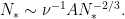
\displaystyle \partial_t \hat u(t,k) + 2\pi \sum_{k = k_1 + k_2} (\hat u(t,k_1) \cdot ik_2) \hat u(t,k_2) =

\displaystyle - 4\pi^2 \nu |k|^2 \hat u(t,k) + 2\pi ik \hat p(t,k) + \hat f(t,k) \ \ \ \ \ (1)


\displaystyle k \cdot \hat u(t,k) = 0.

We may normalise {u} (and {f}) to have mean zero, so that {\hat u(t,0)=0}. Then we introduce the dyadic energies

\displaystyle E_N(t) := \sum_{|k| \sim N} |\hat u(t,k)|^2

where {N \geq 1} ranges over the powers of two, and {|k| \sim N} is shorthand for {N \leq |k| < 2N}. Taking the inner product of (1) with {\hat u(t,k)}, we obtain the energy flow equation

\displaystyle \partial_t E_N = \sum_{N_1,N_2} \Pi_{N,N_1,N_2} - D_N + F_N \ \ \ \ \ (2)


where {N_1,N_2} range over powers of two, {\Pi_{N,N_1,N_2}} is the energy flow rate

\displaystyle \Pi_{N,N_1,N_2} := -2\pi \sum_{k=k_1+k_2: |k| \sim N, |k_1| \sim N_1, |k_2| \sim N_2}

\displaystyle (\hat u(t,k_1) \cdot ik_2) (\hat u(t,k) \cdot \hat u(t,k_2)),

{D_N} is the energy dissipation rate

\displaystyle D_N := 4\pi^2 \nu \sum_{|k| \sim N} |k|^2 |\hat u(t,k)|^2

and {F_N} is the energy injection rate

\displaystyle F_N := \sum_{|k| \sim N} \hat u(t,k) \cdot \hat f(t,k).

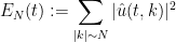
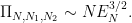
The Navier-Stokes equations are notoriously difficult to solve in general. Despite this, Kolmogorov in 1941 was able to give a convincing heuristic argument for what the distribution of the dyadic energies {E_N} should become over long times, assuming that some sort of distributional steady state is reached. It is common to present this argument in the form of dimensional analysis, but one can also give a more “first principles” form Kolmogorov’s argument, which I will do here. Heuristically, one can divide the frequency scales {N} into three regimes:

  • The injection regime in which the energy injection rate {F_N} dominates the right-hand side of (2);
  • The energy flow regime in which the flow rates {\Pi_{N,N_1,N_2}} dominate the right-hand side of (2); and
  • The dissipation regime in which the dissipation {D_N} dominates the right-hand side of (2).

If we assume a fairly steady and smooth forcing term {f}, then {\hat f} will be supported on the low frequency modes {k=O(1)}, and so we heuristically expect the injection regime to consist of the low scales {N=O(1)}. Conversely, if we take the viscosity {\nu} to be small, we expect the dissipation regime to only occur for very large frequencies {N}, with the energy flow regime occupying the intermediate frequencies.

We can heuristically predict the dividing line between the energy flow regime. Of all the flow rates {\Pi_{N,N_1,N_2}}, it turns out in practice that the terms in which {N_1,N_2 = N+O(1)} (i.e., interactions between comparable scales, rather than widely separated scales) will dominate the other flow rates, so we will focus just on these terms. It is convenient to return back to physical space, decomposing the velocity field {u} into Littlewood-Paley components

\displaystyle u_N(t,x) := \sum_{|k| \sim N} \hat u(t,k) e^{2\pi i k \cdot x}

of the velocity field {u(t,x)} at frequency {N}. By Plancherel’s theorem, this field will have an {L^2} norm of {E_N(t)^{1/2}}, and as a naive model of turbulence we expect this field to be spread out more or less uniformly on the torus, so we have the heuristic

\displaystyle |u_N(t,x)| = O( E_N(t)^{1/2} ),

and a similar heuristic applied to {\nabla u_N} gives

\displaystyle |\nabla u_N(t,x)| = O( N E_N(t)^{1/2} ).

(One can consider modifications of the Kolmogorov model in which {u_N} is concentrated on a lower-dimensional subset of the three-dimensional torus, leading to some changes in the numerology below, but we will not consider such variants here.) Since

\displaystyle \Pi_{N,N_1,N_2} = - \int_{{\bf R}^3/{\bf Z}^3} u_N \cdot ( (u_{N_1} \cdot \nabla) u_{N_2} )\ dx

we thus arrive at the heuristic

\displaystyle \Pi_{N,N_1,N_2} = O( N_2 E_N^{1/2} E_{N_1}^{1/2} E_{N_2}^{1/2} ).

Of course, there is the possibility that due to significant cancellation, the energy flow is significantly less than {O( N E_N(t)^{3/2} )}, but we will assume that cancellation effects are not that significant, so that we typically have

\displaystyle \Pi_{N,N_1,N_2} \sim N_2 E_N^{1/2} E_{N_1}^{1/2} E_{N_2}^{1/2} \ \ \ \ \ (3)


or (assuming that {E_N} does not oscillate too much in {N}, and {N_1,N_2} are close to {N})

\displaystyle \Pi_{N,N_1,N_2} \sim N E_N^{3/2}.

On the other hand, we clearly have

\displaystyle D_N \sim \nu N^2 E_N.

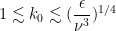
We thus expect to be in the dissipation regime when

\displaystyle N \gtrsim \nu^{-1} E_N^{1/2} \ \ \ \ \ (4)


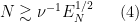
and in the energy flow regime when

\displaystyle 1 \lesssim N \lesssim \nu^{-1} E_N^{1/2}. \ \ \ \ \ (5)


Now we study the energy flow regime further. We assume a “statistically scale-invariant” dynamics in this regime, in particular assuming a power law

\displaystyle E_N \sim A N^{-\alpha} \ \ \ \ \ (6)


for some {A,\alpha > 0}. From (3), we then expect an average asymptotic of the form

\displaystyle \Pi_{N,N_1,N_2} \approx A^{3/2} c_{N,N_1,N_2} (N N_1 N_2)^{1/3 - \alpha/2} \ \ \ \ \ (7)


for some structure constants {c_{N,N_1,N_2} \sim 1} that depend on the exact nature of the turbulence; here we have replaced the factor {N_2} by the comparable term {(N N_1 N_2)^{1/3}} to make things more symmetric. In order to attain a steady state in the energy flow regime, we thus need a cancellation in the structure constants:

\displaystyle \sum_{N_1,N_2} c_{N,N_1,N_2} (N N_1 N_2)^{1/3 - \alpha/2} \approx 0. \ \ \ \ \ (8)


On the other hand, if one is assuming statistical scale invariance, we expect the structure constants to be scale-invariant (in the energy flow regime), in that

\displaystyle c_{\lambda N, \lambda N_1, \lambda N_2} = c_{N,N_1,N_2} \ \ \ \ \ (9)


for dyadic {\lambda > 0}. Also, since the Euler equations conserve energy, the energy flows {\Pi_{N,N_1,N_2}} symmetrise to zero,

\displaystyle \Pi_{N,N_1,N_2} + \Pi_{N,N_2,N_1} + \Pi_{N_1,N,N_2} + \Pi_{N_1,N_2,N} + \Pi_{N_2,N,N_1} + \Pi_{N_2,N_1,N} = 0,

which from (7) suggests a similar cancellation among the structure constants

\displaystyle c_{N,N_1,N_2} + c_{N,N_2,N_1} + c_{N_1,N,N_2} + c_{N_1,N_2,N} + c_{N_2,N,N_1} + c_{N_2,N_1,N} \approx 0.

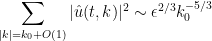
Combining this with the scale-invariance (9), we see that for fixed {N}, we may organise the structure constants {c_{N,N_1,N_2}} for dyadic {N_1,N_2} into sextuples which sum to zero (including some degenerate tuples of order less than six). This will automatically guarantee the cancellation (8) required for a steady state energy distribution, provided that

\displaystyle \frac{1}{3} - \frac{\alpha}{2} = 0

or in other words

\displaystyle \alpha = \frac{2}{3};

for any other value of {\alpha}, there is no particular reason to expect this cancellation (8) to hold. Thus we are led to the heuristic conclusion that the most stable power law distribution for the energies {E_N} is the {2/3} law

\displaystyle E_N \sim A N^{-2/3} \ \ \ \ \ (10)


or in terms of shell energies, we have the famous Kolmogorov 5/3 law

\displaystyle \sum_{|k| = k_0 + O(1)} |\hat u(t,k)|^2 \sim A k_0^{-5/3}.

Given that frequency interactions tend to cascade from low frequencies to high (if only because there are so many more high frequencies than low ones), the above analysis predicts a stablising effect around this power law: scales at which a law (6) holds for some {\alpha > 2/3} are likely to lose energy in the near-term, while scales at which a law (6) hold for some {\alpha< 2/3} are conversely expected to gain energy, thus nudging the exponent of power law towards {2/3}.

We can solve for {A} in terms of energy dissipation as follows. If we let {N_*} be the frequency scale demarcating the transition from the energy flow regime (5) to the dissipation regime (4), we have

\displaystyle N_* \sim \nu^{-1} E_{N_*}

and hence by (10)

\displaystyle N_* \sim \nu^{-1} A N_*^{-2/3}.

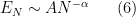
On the other hand, if we let {\epsilon := D_{N_*}} be the energy dissipation at this scale {N_*} (which we expect to be the dominant scale of energy dissipation), we have

\displaystyle \epsilon \sim \nu N_*^2 E_N \sim \nu N_*^2 A N_*^{-2/3}.

Some simple algebra then lets us solve for {A} and {N_*} as

\displaystyle N_* \sim (\frac{\epsilon}{\nu^3})^{1/4}

and

\displaystyle A \sim \epsilon^{2/3}.

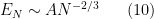
Thus, we have the Kolmogorov prediction

\displaystyle \sum_{|k| = k_0 + O(1)} |\hat u(t,k)|^2 \sim \epsilon^{2/3} k_0^{-5/3}

for

\displaystyle 1 \lesssim k_0 \lesssim (\frac{\epsilon}{\nu^3})^{1/4}

with energy dissipation occuring at the high end {k_0 \sim (\frac{\epsilon}{\nu^3})^{1/4}} of this scale, which is counterbalanced by the energy injection at the low end {k_0 \sim 1} of the scale.

Mathematicians study a variety of different mathematical structures, but perhaps the structures that are most commonly associated with mathematics are the number systems, such as the integers {{\bf Z}} or the real numbers {{\bf R}}. Indeed, the use of number systems is so closely identified with the practice of mathematics that one sometimes forgets that it is possible to do mathematics without explicit reference to any concept of number. For instance, the ancient Greeks were able to prove many theorems in Euclidean geometry, well before the development of Cartesian coordinates and analytic geometry in the seventeenth century, or the formal constructions or axiomatisations of the real number system that emerged in the nineteenth century (not to mention precursor concepts such as zero or negative numbers, whose very existence was highly controversial, if entertained at all, to the ancient Greeks). To do this, the Greeks used geometric operations as substitutes for the arithmetic operations that would be more familiar to modern mathematicians. For instance, concatenation of line segments or planar regions serves as a substitute for addition; the operation of forming a rectangle out of two line segments would serve as a substitute for multiplication; the concept of similarity can be used as a substitute for ratios or division; and so forth.

A similar situation exists in modern physics. Physical quantities such as length, mass, momentum, charge, and so forth are routinely measured and manipulated using the real number system {{\bf R}} (or related systems, such as {{\bf R}^3} if one wishes to measure a vector-valued physical quantity such as velocity). Much as analytic geometry allows one to use the laws of algebra and trigonometry to calculate and prove theorems in geometry, the identification of physical quantities with numbers allows one to express physical laws and relationships (such as Einstein’s famous mass-energy equivalence {E=mc^2}) as algebraic (or differential) equations, which can then be solved and otherwise manipulated through the extensive mathematical toolbox that has been developed over the centuries to deal with such equations.

However, as any student of physics is aware, most physical quantities are not represented purely by one or more numbers, but instead by a combination of a number and some sort of unit. For instance, it would be a category error to assert that the length of some object was a number such as {10}; instead, one has to say something like “the length of this object is {10} yards”, combining both a number {10} and a unit (in this case, the yard). Changing the unit leads to a change in the numerical value assigned to this physical quantity, even though no physical change to the object being measured has occurred. For instance, if one decides to use feet as the unit of length instead of yards, then the length of the object is now {30} feet; if one instead uses metres, the length is now {9.144} metres; and so forth. But nothing physical has changed when performing this change of units, and these lengths are considered all equal to each other:

\displaystyle  10 \hbox{ yards } = 30 \hbox{ feet } = 9.144 \hbox{ metres}.

It is then common to declare that while physical quantities and units are not, strictly speaking, numbers, they should be manipulated using the laws of algebra as if they were numerical quantities. For instance, if an object travels {10} metres in {5} seconds, then its speed should be

\displaystyle  (10 m) / (5 s) = 2 ms^{-1}

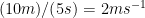
where we use the usual abbreviations of {m} and {s} for metres and seconds respectively. Similarly, if the speed of light {c} is {c=299 792 458 ms^{-1}} and an object has mass {10 kg}, then Einstein’s mass-energy equivalence {E=mc^2} then tells us that the energy-content of this object is

\displaystyle  (10 kg) (299 792 458 ms^{-1})^2 \approx 8.99 \times 10^{17} kg m^2 s^{-2}.

Note that the symbols {kg, m, s} are being manipulated algebraically as if they were mathematical variables such as {x} and {y}. By collecting all these units together, we see that every physical quantity gets assigned a unit of a certain dimension: for instance, we see here that the energy {E} of an object can be given the unit of {kg m^2 s^{-2}} (more commonly known as a Joule), which has the dimension of {M L^2 T^{-2}} where {M, L, T} are the dimensions of mass, length, and time respectively.

There is however one important limitation to the ability to manipulate “dimensionful” quantities as if they were numbers: one is not supposed to add, subtract, or compare two physical quantities if they have different dimensions, although it is acceptable to multiply or divide two such quantities. For instance, if {m} is a mass (having the units {M}) and {v} is a speed (having the units {LT^{-1}}), then it is physically “legitimate” to form an expression such as {\frac{1}{2} mv^2}, but not an expression such as {m+v} or {m-v}; in a similar spirit, statements such as {m=v} or {m\geq v} are physically meaningless. This combines well with the mathematical distinction between vector, scalar, and matrix quantities, which among other things prohibits one from adding together two such quantities if their vector or matrix type are different (e.g. one cannot add a scalar to a vector, or a vector to a matrix), and also places limitations on when two such quantities can be multiplied together. A related limitation, which is not always made explicit in physics texts, is that transcendental mathematical functions such as {\sin} or {\exp} should only be applied to arguments that are dimensionless; thus, for instance, if {v} is a speed, then {\hbox{arctanh}(v)} is not physically meaningful, but {\hbox{arctanh}(v/c)} is (this particular quantity is known as the rapidity associated to this speed).

These limitations may seem like a weakness in the mathematical modeling of physical quantities; one may think that one could get a more “powerful” mathematical framework if one were allowed to perform dimensionally inconsistent operations, such as add together a mass and a velocity, add together a vector and a scalar, exponentiate a length, etc. Certainly there is some precedent for this in mathematics; for instance, the formalism of Clifford algebras does in fact allow one to (among other things) add vectors with scalars, and in differential geometry it is quite common to formally apply transcendental functions (such as the exponential function) to a differential form (for instance, the Liouville measure {\frac{1}{n!} \omega^n} of a symplectic manifold can be usefully thought of as a component of the exponential {\exp(\omega)} of the symplectic form {\omega}).

However, there are several reasons why it is advantageous to retain the limitation to only perform dimensionally consistent operations. One is that of error correction: one can often catch (and correct for) errors in one’s calculations by discovering a dimensional inconsistency, and tracing it back to the first step where it occurs. Also, by performing dimensional analysis, one can often identify the form of a physical law before one has fully derived it. For instance, if one postulates the existence of a mass-energy relationship involving only the mass of an object {m}, the energy content {E}, and the speed of light {c}, dimensional analysis is already sufficient to deduce that the relationship must be of the form {E = \alpha mc^2} for some dimensionless absolute constant {\alpha}; the only remaining task is then to work out the constant of proportionality {\alpha}, which requires physical arguments beyond that provided by dimensional analysis. (This is a simple instance of a more general application of dimensional analysis known as the Buckingham {\pi} theorem.)

The use of units and dimensional analysis has certainly been proven to be very effective tools in physics. But one can pose the question of whether it has a properly grounded mathematical foundation, in order to settle any lingering unease about using such tools in physics, and also in order to rigorously develop such tools for purely mathematical purposes (such as analysing identities and inequalities in such fields of mathematics as harmonic analysis or partial differential equations).

The example of Euclidean geometry mentioned previously offers one possible approach to formalising the use of dimensions. For instance, one could model the length of a line segment not by a number, but rather by the equivalence class of all line segments congruent to the original line segment (cf. the Frege-Russell definition of a number). Similarly, the area of a planar region can be modeled not by a number, but by the equivalence class of all regions that are equidecomposable with the original region (one can, if one wishes, restrict attention here to measurable sets in order to avoid Banach-Tarski-type paradoxes, though that particular paradox actually only arises in three and higher dimensions). As mentioned before, it is then geometrically natural to multiply two lengths to form an area, by taking a rectangle whose line segments have the stated lengths, and using the area of that rectangle as a product. This geometric picture works well for units such as length and volume that have a spatial geometric interpretation, but it is less clear how to apply it for more general units. For instance, it does not seem geometrically natural (or, for that matter, conceptually helpful) to envision the equation {E=mc^2} as the assertion that the energy {E} is the volume of a rectangular box whose height is the mass {m} and whose length and width is given by the speed of light {c}.

But there are at least two other ways to formalise dimensionful quantities in mathematics, which I will discuss below the fold. The first is a “parametric” model in which dimensionful objects are modeled as numbers (or vectors, matrices, etc.) depending on some base dimensional parameters (such as units of length, mass, and time, or perhaps a coordinate system for space or spacetime), and transforming according to some representation of a structure group that encodes the range of these parameters; this type of “coordinate-heavy” model is often used (either implicitly or explicitly) by physicists in order to efficiently perform calculations, particularly when manipulating vector or tensor-valued quantities. The second is an “abstract” model in which dimensionful objects now live in an abstract mathematical space (e.g. an abstract vector space), in which only a subset of the operations available to general-purpose number systems such as {{\bf R}} or {{\bf R}^3} are available, namely those operations which are “dimensionally consistent” or invariant (or more precisely, equivariant) with respect to the action of the underlying structure group. This sort of “coordinate-free” approach tends to be the one which is preferred by pure mathematicians, particularly in the various branches of modern geometry, in part because it can lead to greater conceptual clarity, as well as results of great generality; it is also close to the more informal practice of treating mathematical manipulations that do not preserve dimensional consistency as being physically meaningless.

Read the rest of this entry »

In harmonic analysis and PDE, one often wants to place a function f: {\bf R}^d \to {\bf C} on some domain (let’s take a Euclidean space {\bf R}^d for simplicity) in one or more function spaces in order to quantify its “size” in some sense.  Examples include

  • The Lebesgue spaces L^p of functions f whose norm \|f\|_{L^p} := (\int_{{\bf R}^d} |f|^p)^{1/p} is finite, as well as their relatives such as the weak L^p spaces L^{p,\infty} (and more generally the Lorentz spaces L^{p,q}) and Orlicz spaces such as L \log L and e^L;
  • The classical regularity spaces C^k, together with their Hölder continuous counterparts C^{k,\alpha};
  • The Sobolev spaces W^{s,p} of functions f whose norm \|f\|_{W^{s,p}} = \|f\|_{L^p} + \| |\nabla|^s f\|_{L^p} is finite (other equivalent definitions of this norm exist, and there are technicalities if s is negative or p \not \in (1,\infty)), as well as relatives such as homogeneous Sobolev spaces \dot W^{s,p}, Besov spaces B^{s,p}_q, and Triebel-Lizorkin spaces F^{s,p}_q.  (The conventions for the superscripts and subscripts here are highly variable.)
  • Hardy spaces {\mathcal H}^p, the space BMO of functions of bounded mean oscillation (and the subspace VMO of functions of vanishing mean oscillation);
  • The Wiener algebra A;
  • Morrey spaces M^p_q;
  • The space M of finite measures;
  • etc., etc.

As the above partial list indicates, there is an entire zoo of function spaces one could consider, and it can be difficult at first to see how they are organised with respect to each other.  However, one can get some clarity in this regard by drawing a type diagram for the function spaces one is trying to study.  A type diagram assigns a tuple (usually a pair) of relevant exponents to each function space.  For function spaces X on Euclidean space, two such exponents are the regularity s of the space, and the integrability p of the space.  These two quantities are somewhat fuzzy in nature (and are not easily defined for all possible function spaces), but can basically be described as follows.  We test the function space norm \|f\|_X of a modulated rescaled bump function

f(x) := A e^{i x \cdot \xi} \phi( \frac{x-x_0}{R} ) (1)

where A > 0 is an amplitude, R > 0 is a radius, \phi \in C^\infty_c({\bf R}^d) is a test function, x_0 is a position, and \xi \in {\bf R}^d is a frequency of some magnitude |\xi| \sim N.  One then studies how the norm \|f\|_X depends on the parameters A, R, N.  Typically, one has a relationship of the form

\|f\|_X \sim A N^s R^{d/p} (2)

for some exponents s, p, at least in the high-frequency case when N is large (in particular, from the uncertainty principle it is natural to require N \gtrsim 1/R, and when dealing with inhomogeneous norms it is also natural to require N \gtrsim 1).  The exponent s measures how sensitive the X norm is to oscillation, and thus controls regularity; if s is large, then oscillating functions will have large X norm, and thus functions in X will tend not to oscillate too much and thus be smooth.    Similarly, the exponent p measures how sensitive the X norm is to the function f spreading out to large scales; if p is small, then slowly decaying functions will have large norm, so that functions in X tend to decay quickly; conversely, if p is large, then singular functions will tend to have large norm, so that functions in X will tend to not have high peaks.

Note that the exponent s in (2) could be positive, zero, or negative, however the exponent p should be non-negative, since intuitively enlarging R should always lead to a larger (or at least comparable) norm.  Finally, the exponent in the A parameter should always be 1, since norms are by definition homogeneous.  Note also that the position x_0 plays no role in (1); this reflects the fact that most of the popular function spaces in analysis are translation-invariant.

The type diagram below plots the s, 1/p indices of various spaces.  The black dots indicate those spaces for which the s, 1/p indices are fixed; the blue dots are those spaces for which at least one of the s, 1/p indices are variable (and so, depending on the value chosen for these parameters, these spaces may end up in a different location on the type diagram than the typical location indicated here).

(There are some minor cheats in this diagram, for instance for the Orlicz spaces L \log L and e^L one has to adjust (1) by a logarithmic factor.   Also, the norms for the Schwartz space {\mathcal S} are not translation-invariant and thus not perfectly describable by this formalism. This picture should be viewed as a visual aid only, and not as a genuinely rigorous mathematical statement.)

The type diagram can be used to clarify some of the relationships between function spaces, such as Sobolev embedding.  For instance, when working with inhomogeneous spaces (which basically identifies low frequencies N \ll 1 with medium frequencies N \sim 1, so that one is effectively always in the regime N \gtrsim 1), then decreasing the s parameter results in decreasing the right-hand side of (1).  Thus, one expects the function space norms to get smaller (and the function spaces to get larger) if one decreases s while keeping p fixed.  Thus, for instance, W^{k,p} should be contained in W^{k-1,p}, and so forth.  Note however that this inclusion is not available for homogeneous function spaces such as \dot W^{k,p}, in which the frequency parameter N can be either much larger than 1 or much smaller than 1.

Similarly, if one is working in a compact domain rather than in {\bf R}^d, then one has effectively capped the radius parameter R to be bounded, and so we expect the function space norms to get smaller (and the function spaces to get larger) as one increases 1/p, thus for instance L^2 will be contained in L^1.  Conversely, if one is working in a discrete domain such as {\Bbb Z}^d, then the radius parameter R has now effectively been bounded from below, and the reverse should occur: the function spaces should get larger as one decreases 1/p.  (If the domain is both compact and discrete, then it is finite, and on a finite-dimensional space all norms are equivalent.)

As mentioned earlier, the uncertainty principle suggests that one has the restriction N \gtrsim 1/R.  From this and (2), we expect to be able to enlarge the function space by trading in the regularity parameter s for the integrability parameter p, keeping the dimensional quantity d/p - s fixed.  This is indeed how Sobolev embedding works.   Note in some cases one runs out of regularity before p goes all the way to infinity (thus ending up at an L^p space), while in other cases p hits infinity first.  In the latter case, one can embed the Sobolev space into a Holder space such as C^{k,\alpha}.

On continuous domains, one can send the frequency N off to infinity, keeping the amplitude A and radius R fixed.  From this and (1) we see that norms with a lower regularity s can never hope to control norms with a higher regularity s' > s, no matter what one does with the integrability parameter.   Note however that in discrete settings this obstruction disappears; when working on, say, {\bf Z}^d, then in fact one can gain as much regularity as one wishes for free, and there is no distinction between a Lebesgue space \ell^p and their Sobolev counterparts W^{k,p} in such a setting.

When interpolating between two spaces (using either the real or complex interpolation method), the interpolated space usually has regularity and integrability exponents on the line segment between the corresponding exponents of the endpoint spaces.  (This can be heuristically justified from the formula (2) by thinking about how the real or complex interpolation methods actually work.)  Typically, one can control the norm of the interpolated space by the geometric mean of the endpoint norms that is indicated by this line segment; again, this is plausible from looking at (2).

The space L^2 is self-dual.  More generally, the dual of a function space X will generally have type exponents that are the reflection of the original exponents around the L^2 origin.  Consider for instance the dual spaces H^s, H^{-s} or {\mathcal H}^1, BMO in the above diagram.

Spaces whose integrability exponent p is larger than 1 (i.e. which lie to the left of the dotted line) tend to be Banach spaces, while spaces whose integrability exponent is less than 1 are almost never Banach spaces.  (This can be justified by covering a large ball into small balls and considering how (1) would interact with the triangle inequality in this case).  The case p=1 is borderline; some spaces at this level of integrability, such as L^1, are Banach spaces, while other spaces, such as L^{1,\infty}, are not.

While the regularity s and integrability p are usually the most important exponents in a function space (because amplitude, width, and frequency are usually the most important features of a function in analysis), they do not tell the entire story.  One major reason for this is that the modulated bump functions (1), while an important class of test examples of functions, are by no means the only functions that one would wish to study.  For instance, one could also consider sums of bump functions (1) at different scales.  The behaviour of the function space norms on such spaces is often controlled by secondary exponents, such as the second exponent q that arises in Lorentz spaces, Besov spaces, or Triebel-Lizorkin spaces.  For instance, consider the function

f_M(x) := \sum_{m=1}^M 2^{-md} \phi(x/2^m), (3)

where M is a large integer, representing the number of distinct scales present in f_M.  Any function space with regularity s=0 and p=1 should assign each summand 2^{-md} \phi(x/2^m) in (3) a norm of O(1), so the norm of f_M could be as large as O(M) if one assumes the triangle inequality.  This is indeed the case for the L^1 norm, but for the weak L^1 norm, i.e. the L^{1,\infty} norm,  f_M only has size O(1).  More generally, for the Lorentz spaces L^{1,q}, f_M will have a norm of about O(M^{1/q}).   Thus we see that such secondary exponents can influence the norm of a function by an amount which is polynomial in the number of scales.  In many applications, though, the number of scales is a “logarithmic” quantity and thus of lower order interest when compared against the “polynomial” exponents such as s and p.  So the fine distinctions between, say, strong L^1 and weak L^1, are only of interest in “critical” situations in which one cannot afford to lose any logarithmic factors (this is for instance the case in much of Calderon-Zygmund theory).

We have cheated somewhat by only working in the high frequency regime.  When dealing with inhomogeneous spaces, one often has a different set of exponents for (1) in the low-frequency regime than in the high-frequency regime.  In such cases, one sometimes has to use a more complicated type diagram to  genuinely model the situation, e.g. by assigning to each space a convex set of type exponents rather than a single exponent, or perhaps having two separate type diagrams, one for the high frequency regime and one for the low frequency regime.   Such diagrams can get quite complicated, and will probably not be much use to a beginner in the subject, though in the hands of an expert who knows what he or she is doing, they can still be an effective visual aid.

Archives