Counting the number of solutions to the Erdös-Straus equation on unit fractions

Christian Elsholtz and I have recently finished our joint paper “Counting the number of solutions to the Erdös-Straus equation on unit fractions“, submitted to the Journal of the Australian Mathematical Society. This supercedes my previous paper on the subject, by obtaining stronger and more general results. (The paper is currently in the process of being resubmitted to the arXiv, and should appear at this link within a few days.)

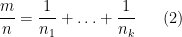
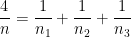
As with the previous paper, the main object of study is the number of solutions to the Diophantine equation

with positive integers. The Erdös-Straus conjecture asserts that for all . Since for all positive integers , it suffices to show that for all primes .

We single out two special types of solutions: Type I solutions, in which is divisible by and are coprime to , and Type II solutions, in which is coprime to and are divisible by . Let denote the number of Type I and Type II solutions respectively. For any , one has

with equality when is an odd primes . Thus, to prove the Erdös-Strauss conjecture, it suffices to show that at least one of , is positive whenever is an odd prime.

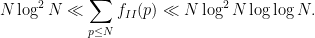
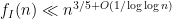
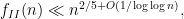
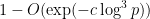
Our first main results are the asymptotics

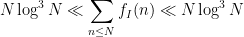
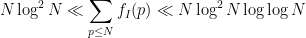
This improves upon the results in the previous paper, which only established

and

The double logarithmic factor in the upper bound for is artificial (arising from the inefficiency in the Brun-Titchmarsh inequality on very short progressions) but we do not know how to remove it.

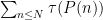
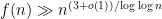
The methods are similar to those in the previous paper (which were also independently discovered in unpublished work of Elsholtz and Heath-Brown), but with the additional input of the Erdös divisor bound on expressions of the form for polynomials , discussed in this recent blog post. (Actually, we need to tighten Erdös’ bound somewhat, to obtain some uniformity in the bounds even as the coefficients of become large, but this turns out to be achievable by going through the original arguments of Erdös more carefully.)

We also note an observation of Heath-Brown, that in our notation gives the lower bound

thus, we see that for typical , that most solutions to the Erdös-Straus equation are not of Type I or Type II, in contrast to the case when is prime.

We also have a number other new results. We find a way to systematically unify all the previously known parameterisations of solutions to the Erdös-Straus equation, by lifting the Cayley-type surface to a certain three-dimensional variety in six-dimensional affine space, in such a way that integer points in the former arise from integer points in the latter. Each of the previously known characterisations of solutions then corresponds to a different choice of coordinates on this variety. (This point of view was also adopted in a paper of Heath-Brown, who interprets this lifted variety as the universal torsor of the Cayley surface.) By optimising between these parameterisations and exploiting the divisor bound, we obtain some bounds on the worst-case behaviour of and , namely

and

which should be compared to a recent previous bound 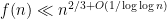of Browning and Elsholtz. In the other direction, we show that for infinitely many , and for almost all primes . Here, the main tools are some bounds for the representation of a rational as a sum of two unit fractions in the above-mentioned work of Browning and Elsholtz, and also the Turán-Kubilius inequality.

We also completely classify all the congruence classes that can be solved by polynomials, completing the partial list discussed in the previous post. Specifically, the Erdös-Straus conjecture is true for whenever one of the following congruence-type conditions is satisfied:

1. , where are such that .
2. and , where are such that .
3. and , where are such that .
4. or , where are such that and .
5. , where are such that .
6. , where are such that .

In principle, this suggests a way to extend the existing verification of the Erdös-Straus conjecture beyond the current range of by collecting all congruences to small moduli (e.g. up to ), and then using this to sieve out the primes up to a given size.

Finally, we begin a study of the more general equation

where are fixed. We can obtain a partial analogue of our main bounds for the case, namely that

and

were denotes the number of solutions to (2) which are of “Type II” in the sense that are all divisible by . However, we do not believe our bounds to be sharp in the large regime, though it does show that the expected number of solutions to (2) should grow rapidly in .

Erdos’ divisor bound

One of the basic problems in analytic number theory is to obtain bounds and asymptotics for sums of the form

in the limit , where ranges over natural numbers less than , and is some arithmetic function of number-theoretic interest. (It is also often convenient to replace this sharply truncated sum with a smoother sum such as , but we will not discuss this technicality here.) For instance, the prime number theorem is equivalent to the assertion

where is the von Mangoldt function, while the Riemann hypothesis is equivalent to the stronger assertion

It is thus of interest to develop techniques to estimate such sums . Of course, the difficulty of this task depends on how “nice” the function is. The functions that come up in number theory lie on a broad spectrum of “niceness”, with some particularly nice functions being quite easy to sum, and some being insanely difficult.

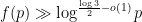
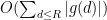
At the easiest end of the spectrum are those functions that exhibit some sort of regularity or “smoothness”. Examples of smoothness include “Archimedean” smoothness, in which is the restriction of some smooth function from the reals to the natural numbers, and the derivatives of are well controlled. A typical example is

One can already get quite good bounds on this quantity by comparison with the integral , namely

with sharper bounds available by using tools such as the Euler-Maclaurin formula (see this blog post). Exponentiating such asymptotics, incidentally, leads to one of the standard proofs of Stirling’s formula (as discussed in this blog post).

One can also consider “non-Archimedean” notions of smoothness, such as periodicity relative to a small period . Indeed, if is periodic with period (and is thus essentially a function on the cyclic group ), then one has the easy bound

In particular, we have the fundamental estimate

This is a good estimate when is much smaller than , but as approaches in magnitude, the error term begins to overwhelm the main term , and one needs much more delicate information on the fractional part of in order to obtain good estimates at this point.

One can also consider functions which combine “Archimedean” and “non-Archimedean” smoothness into an “adelic” smoothness. We will not define this term precisely here (though the concept of a Schwartz-Bruhat function is one way to capture this sort of concept), but a typical example might be

where is periodic with some small period . By using techniques such as summation by parts, one can estimate such sums using the techniques used to estimate sums of periodic functions or functions with (Archimedean) smoothness.

Another class of functions that is reasonably well controlled are the multiplicative functions, in which whenever are coprime. Here, one can use the powerful techniques of multiplicative number theory, for instance by working with the Dirichlet series

which are clearly related to the partial sums (essentially via the Mellin transform, a cousin of the Fourier and Laplace transforms); for this post we ignore the (important) issue of how to make sense of this series when it is not absolutely convergent (but see this previous blog post for more discussion). A primary reason that this technique is effective is that the Dirichlet series of a multiplicative function factorises as an Euler product

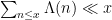
One also obtains similar types of representations for functions that are not quite multiplicative, but are closely related to multiplicative functions, such as the von Mangoldt function (whose Dirichlet series is not given by an Euler product, but instead by the logarithmic derivative of an Euler product).

Moving another notch along the spectrum between well-controlled and ill-controlled functions, one can consider functions that are divisor sums such as

for some other arithmetic function , and some level . This is a linear combination of periodic functions and is thus technically periodic in (with period equal to the least common multiple of all the numbers from to ), but in practice this periodic is far too large to be useful (except for extremely small levels , e.g. ). Nevertheless, we can still control the sum simply by rearranging the summation:

and thus by (1) one can bound this by the sum of a main term and an error term . As long as the level is significantly less than , one may expect the main term to dominate, and one can often estimate this term by a variety of techniques (for instance, if is multiplicative, then multiplicative number theory techniques are quite effective, as mentioned previously). Similarly for other slight variants of divisor sums, such as expressions of the form

or expressions of the form

where each is periodic with period .

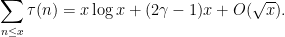
One of the simplest examples of this comes when estimating the divisor function

which counts the number of divisors up to . This is a multiplicative function, and is therefore most efficiently estimated using the techniques of multiplicative number theory; but for reasons that will become clearer later, let us “forget” the multiplicative structure and estimate the above sum by more elementary methods. By applying the preceding method, we see that

Here, we are (barely) able to keep the error term smaller than the main term; this is right at the edge of the divisor sum method, because the level in this case is equal to . Unfortunately, at this high choice of level, it is not always possible to always keep the error term under control like this. For instance, if one wishes to use the standard divisor sum representation

where is the Möbius function, to compute , then one ends up looking at

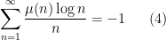
From Dirichlet series methods, it is not difficult to establish the identities

and

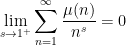
This suggests (but does not quite prove) that one has

and

in the sense of conditionally convergent series. Assuming one can justify this (which, ultimately, requires one to exclude zeroes of the Riemann zeta function on the line , as discussed in this previous post), one is eventually left with the estimate , which is useless as a lower bound (and recovers only the classical Chebyshev estimate as the upper bound). The inefficiency here when compared to the situation with the divisor function can be attributed to the signed nature of the Möbius function , which causes some cancellation in the divisor sum expansion that needs to be compensated for with improved estimates.

However, there are a number of tricks available to reduce the level of divisor sums. The simplest comes from exploiting the change of variables , which can in principle reduce the level by a square root. For instance, when computing the divisor function , one can observe using this change of variables that every divisor of above is paired with one below , and so we have

except when is a perfect square, in which case one must subtract one from the right-hand side. Using this reduced-level divisor sum representation, one can obtain an improvement to (2), namely

This type of argument is also known as the Dirichlet hyperbola method. A variant of this argument can also deduce the prime number theorem from (3), (4) (and with some additional effort, one can even drop the use of (4)); this is discussed at this previous blog post.

Using this square root trick, one can now also control divisor sums such as

(Note that has no multiplicativity properties in , and so multiplicative number theory techniques cannot be directly applied here.) The level of the divisor sum here is initially of order , which is too large to be useful; but using the square root trick, we can expand this expression as

which one can rewrite as

The constraint is periodic in with period , so we can write this as

where is the number of solutions in to the equation , and so

The function is multiplicative, and can be easily computed at primes and prime powers using tools such as quadratic reciprocity and Hensel’s lemma. For instance, by Fermat’s two-square theorem, is equal to for and for . From this and standard multiplicative number theory methods (e.g. by obtaining asymptotics on the Dirichlet series ), one eventually obtains the asymptotic

and also

and thus

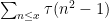
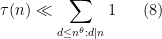
Similar arguments give asymptotics for on other quadratic polynomials; see for instance this paper of Hooley and these papers by McKee. Note that the irreducibility of the polynomial will be important. If one considers instead a sum involving a reducible polynomial, such as , then the analogous quantity becomes significantly larger, leading to a larger growth rate (of order rather than ) for the sum.

However, the square root trick is insufficient by itself to deal with higher order sums involving the divisor function, such as

the level here is initially of order , and the square root trick only lowers this to about , creating an error term that overwhelms the main term. And indeed, the asymptotic for such this sum has not yet been rigorously established (although if one heuristically drops error terms, one can arrive at a reasonable conjecture for this asymptotic), although some results are known if one averages over additional parameters (see e.g. this paper of Greaves, or this paper of Matthiesen).

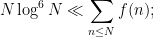
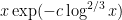
Nevertheless, there is an ingenious argument of Erdös that allows one to obtain good upper and lower bounds for these sorts of sums, in particular establishing the asymptotic

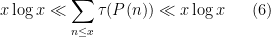
for any fixed irreducible non-constant polynomial that maps to (with the implied constants depending of course on the choice of ). There is also the related moment bound

for any fixed (not necessarily irreducible) and any fixed , due to van der Corput; this bound is in fact used to dispose of some error terms in the proof of (6). These should be compared with what one can obtain from the divisor bound and the trivial bound , giving the bounds

for any fixed .

The lower bound in (6) is easy, since one can simply lower the level in (5) to obtain the lower bound

for any , and the preceding methods then easily allow one to obtain the lower bound by taking small enough (more precisely, if has degree , one should take equal to or less). The upper bounds in (6) and (7) are more difficult. Ideally, if we could obtain upper bounds of the form

for any fixed , then the preceding methods would easily establish both results. Unfortunately, this bound can fail, as illustrated by the following example. Suppose that is the product of distinct primes , each of which is close to . Then has divisors, with of them close to for each . One can think of (the logarithms of) these divisors as being distributed according to what is essentially a Bernoulli distribution, thus a randomly selected divisor of has magnitude about , where is a random variable which has the same distribution as the number of heads in independently tossed fair coins. By the law of large numbers, should concentrate near when is large, which implies that the majority of the divisors of will be close to . Sending , one can show that the bound (8) fails whenever .

This however can be fixed in a number of ways. First of all, even when , one can show weaker substitutes for (8). For instance, for any fixed and one can show a bound of the form

for some depending only on . This nice elementary inequality (first observed by Landreau) already gives a quite short proof of van der Corput’s bound (7).

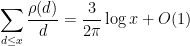
For Erdös’s upper bound (6), though, one cannot afford to lose these additional factors of , and one must argue more carefully. Here, the key observation is that the counterexample discussed earlier – when the natural number is the product of a large number of fairly small primes – is quite atypical; most numbers have at least one large prime factor. For instance, the number of natural numbers less than that contain a prime factor between and is equal to

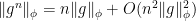
which, thanks to Mertens’ theorem

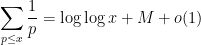
for some absolute constant , is comparable to . In a similar spirit, one can show by similarly elementary means that the number of natural numbers less than that are -smooth, in the sense that all prime factors are at most , is only about or so. Because of this, one can hope that the bound (8), while not true in full generality, will still be true for most natural numbers , with some slightly weaker substitute available (such as (7)) for the exceptional numbers . This turns out to be the case by an elementary but careful argument.

The Erdös argument is quite robust; for instance, the more general inequality

for fixed irreducible and , which improves van der Corput’s inequality (8) was shown by Delmer using the same methods. (A slight error in the original paper of Erdös was also corrected in this latter paper.) In a forthcoming revision to my paper on the Erdös-Straus conjecture, Christian Elsholtz and I have also applied this method to obtain bounds such as

which turn out to be enough to obtain the right asymptotics for the number of solutions to the equation .

Below the fold I will provide some more details of the arguments of Landreau and of Erdös.

Mini-polymath3 discussion thread

I’ve just opened the research thread for the mini-polymath3 project over at the polymath blog.  I decided to use Q2 of this year’s IMO, in part to see how the polymath format copes with a geometric problem.  (The full list of questions for this year is available here.)

This post will serve as the discussion thread of the project, intended to focus all the non-research aspects of the project such as organisational matters or commentary on the progress of the project.    The third component of the project is the wiki page, which is intended to summarise the progress made so far on the problem.

As with mini-polymath1 and mini-polymath2, I myself will be serving primarily as a moderator, and hope other participants will take the lead in the research and in keeping the wiki up-to-date.

Mini-polymath3 begins in 24 hours

Just a reminder that the mini-polymath3 project begins in 24 hours, on July 19, 8pm UTC.

Pappus’s theorem and elliptic curves

An algebraic (affine) plane curve of degree over some field is a curve of the form

where is some non-constant polynomial of degree . Examples of low-degree plane curves include

• Degree (linear) curves , which are simply the lines;
• Degree (quadric) curves , which (when ) include the classical conic sections (i.e. ellipses, hyperbolae, and parabolae), but also include the reducible example of the union of two lines; and
• Degree (cubic) curves , which include the elliptic curves (with non-zero discriminant , so that the curve is smooth) as examples (ignoring some technicalities when has characteristic two or three), but also include the reducible examples of the union of a line and a conic section, or the union of three lines.
• etc.

Algebraic affine plane curves can also be extended to the projective plane by homogenising the polynomial. For instance, the affine quadric curve would become .

One of the fundamental theorems about algebraic plane curves is Bézout’s theorem, which asserts that if a degree curve and a degree curve have no common component, then they intersect in at most points (and if the underlying field is algebraically closed, one works projectively, and one counts intersections with multiplicity, they intersect in exactly points). Thus, for instance, two distinct lines intersect in at most one point; a line and a conic section intersect in at most two points; two distinct conic sections intersect in at most four points; a line and an elliptic curve intersect in at most three points; two distinct elliptic curves intersect in at most nine points; and so forth. Bézout’s theorem is discussed in this previous post.

From linear algebra we also have the fundamental fact that one can build algebraic curves through various specified points. For instance, for any two points one can find a line passing through the points , because this imposes two linear constraints on three unknowns and is thus guaranteed to have at least one solution. Similarly, given any five points , one can find a quadric curve passing through these five points (though note that if three of these points are collinear, then this curve cannot be a conic thanks to Bézout’s theorem, and is thus necessarily reducible to the union of two lines); given any nine points , one can find a cubic curve going through these nine points; and so forth. This simple observation is one of the foundational building blocks of the polynomial method in combinatorial incidence geometry, discussed in these blog posts.

In the degree case, it is always true that two distinct points determine exactly one line . In higher degree, the situation is a bit more complicated. For instance, five collinear points determine more than one quadric curve, as one can simply take the union of the line containing those five points, together with an arbitrary additional line. Similarly, eight points on a conic section plus one additional point determine more than one cubic curve, as one can take that conic section plus an arbitrary line going through the additional point. However, if one places some “general position” hypotheses on these points, then one can recover uniqueness. For instance, given five points, no three of which are collinear, there can be at most one quadric curve that passes through these points (because these five points cannot lie on the union of two lines, and by Bézout’s theorem they cannot simultaneously lie on two distinct conic sections).

For cubic curves, the situation is more complicated still. Consider for instance two distinct cubic curves and that intersect in precisely nine points (note from Bézout’s theorem that this is an entirely typical situation). Then there is in fact an entire one-parameter family of cubic curves that pass through these points, namely the curves for any (with the convention that the constraint is interpreted as when ).

In fact, these are the only cubics that pass through these nine points, or even through eight of the nine points. More precisely, we have the following useful fact, known as the Cayley-Bacharach theorem:

Proposition 1 (Cayley-Bacharach theorem) Let and be two cubic curves that intersect (over some algebraically closed field ) in precisely nine distinct points . Let be a cubic polynomial that vanishes on eight of these points (say ). Then is a linear combination of , and in particular vanishes on the ninth point .

Proof: (This proof is based off of a text of Husemöller.) We assume for contradiction that there is a cubic polynomial that vanishes on , but is not a linear combination of and .

We first make some observations on the points . No four of these points can be collinear, because then by Bézout’s theorem, and would both have to vanish on this line, contradicting the fact that meet in at most nine points. For similar reasons, no seven of these points can lie on a quadric curve.

One consequence of this is that any five of the determine a unique quadric curve . The existence of the curve follows from linear algebra as discussed previously. If five of the points lie on two different quadric curves , then by Bezout’s theorem, they must share a common line; but this line can contain at most three of the five points, and the other two points determine uniquely the other line that is the component of both and , and the claim follows.

Now suppose that three of the first eight points, say , are collinear, lying on a line . The remaining five points do not lie on , and determine a unique quadric curve by the previous discussion. Let be another point on , and let be a point that does not lie on either or . By linear algebra, one can find a non-trivial linear combination of that vanishes at both and . Then is a cubic polynomial that vanishes on the four collinear points and thus vanishes on , thus the cubic curve defined by consists of and a quadric curve. This curve passes through and thus equals . But then does not lie on either or despite being a vanishing point of , a contradiction. Thus, no three points from are collinear.

In a similar vein, suppose next that six of the first eight points, say , lie on a quadric curve ; as no three points are collinear, this quadric curve cannot be the union of two lines, and is thus a conic section. The remaining two points determine a unique line . Let be another point on , and let be another point that does not lie on either and . As before, we can find a non-trivial cubic that vanishes at both . As vanishes at seven points of a conic section , it must vanish on all of , and so the cubic curve defined by is the union of and a line that passes through and , which must necessarily be . But then this curve does not pass through , a contradiction. Thus no six points in lie on a quadric curve.

Finally, let be the line through the two points , and the quadric curve through the five points ; as before, must be a conic section, and by the preceding paragraphs we see that does not lie on either or . We pick two more points lying on but not on . As before, we can find a non-trivial cubic that vanishes on ; it vanishes on four points on and thus defines a cubic curve that consists of and a quadric curve. The quadric curve passes through and is thus ; but then the curve does not pass through , a contradiction. This contradiction finishes the proof of the proposition.

I recently learned of this proposition and its role in unifying many incidence geometry facts concerning lines, quadric curves, and cubic curves. For instance, we can recover the proof of the classical theorem of Pappus:

Theorem 2 (Pappus’ theorem) Let be two distinct lines, let be distinct points on that do not lie on , and let be distinct points on that do not lie on . Suppose that for , the lines and meet at a point . Then the points are collinear.

Proof: We may assume that are distinct, since the claim is trivial otherwise.

Let be the union of the three lines , , and (the purple lines in the first figure), let be the union of the three lines , , and (the dark blue lines), and let be the union of the three lines , , and (the other three lines). By construction, and are cubic curves with no common component that meet at the nine points . Also, is a cubic curve that passes through the first eight of these points, and thus also passes through the ninth point , by the Cayley-Bacharach theorem. The claim follows (note that cannot lie on or ).

The same argument gives the closely related theorem of Pascal:

Theorem 3 (Pascal’s theorem) Let be distinct points on a conic section . Suppose that for , the lines and meet at a point . Then the points are collinear.

Proof: Repeat the proof of Pappus’ theorem, with taking the place of . (Note that as any line meets in at most two points, the cannot lie on .)

One can view Pappus’s theorem as the degenerate case of Pascal’s theorem, when the conic section degenerates to the union of two lines.

Finally, Proposition 1 gives the associativity of the elliptic curve group law:

Theorem 4 (Associativity of the elliptic curve law) Let be a (projective) elliptic curve, where is the point at infinity on the -axis, and the discriminant is non-zero. Define an addition law on by defining to equal , where is the unique point on collinear with and (if are disjoint) or tangent to (if ), and is the reflection of through the -axis (thus are collinear), with the convention . Then gives the structure of an abelian group with identity and inverse .

Proof: It is clear that is the identity for , is an inverse, and is abelian. The only non-trivial assertion is associativity: . By a perturbation (or Zariski closure) argument, we may assume that we are in the generic case when are all distinct from each other and from . (Here we are implicitly using the smoothness of the elliptic curve, which is guaranteed by the hypothesis that the discriminant is non-zero.)

Let be the union of the three lines , , and (the purple lines), and let be the union of the three lines , , and (the green lines). Observe that and are cubic curves with no common component that meet at the nine distinct points . The cubic curve goes through the first eight of these points, and thus (by Proposition 1) also goes through the ninth point . This implies that the line through and meets in both and , and so these two points must be equal, and so as required.

One can view Pappus’s theorem and Pascal’s theorem as a degeneration of the associativity of the elliptic curve law, when the elliptic curve degenerates to three lines (in the case of Pappus) or the union of one line and one conic section (in the case of Pascal’s theorem).

Gleason’s lemma

This is another installment of my my series of posts on Hilbert’s fifth problem. One formulation of this problem is answered by the following theorem of Gleason and Montgomery-Zippin:

Theorem 1 (Hilbert’s fifth problem) Let be a topological group which is locally Euclidean. Then is isomorphic to a Lie group.

Theorem 1 is deep and difficult result, but the discussion in the previous posts has reduced the proof of this Theorem to that of establishing two simpler results, involving the concepts of a no small subgroups (NSS) subgroup, and that of a Gleason metric. We briefly recall the relevant definitions:

Definition 2 (NSS) A topological group is said to have no small subgroups, or is NSS for short, if there is an open neighbourhood of the identity in that contains no subgroups of other than the trivial subgroup .

Definition 3 (Gleason metric) Let be a topological group. A Gleason metric on is a left-invariant metric which generates the topology on and obeys the following properties for some constant , writing for :

• (Escape property) If and is such that , then

  

• (Commutator estimate) If are such that , then

  

  where is the commutator of and .

The remaining steps in the resolution of Hilbert’s fifth problem are then as follows:

Theorem 4 (Reduction to the NSS case) Let be a locally compact group, and let be an open neighbourhood of the identity in . Then there exists an open subgroup of , and a compact subgroup of contained in , such that is NSS and locally compact.

Theorem 5 (Gleason’s lemma) Let be a locally compact NSS group. Then has a Gleason metric.

The purpose of this post is to establish these two results, using arguments that are originally due to Gleason. We will split this task into several subtasks, each of which improves the structure on the group by some amount:

Proposition 6 (From locally compact to metrisable) Let be a locally compact group, and let be an open neighbourhood of the identity in . Then there exists an open subgroup of , and a compact subgroup of contained in , such that is locally compact and metrisable.

For any open neighbourhood of the identity in , let be the union of all the subgroups of that are contained in . (Thus, for instance, is NSS if and only if is trivial for all sufficiently small .)

Proposition 7 (From metrisable to subgroup trapping) Let be a locally compact metrisable group. Then has the subgroup trapping property: for every open neighbourhood of the identity, there exists another open neighbourhood of the identity such that generates a subgroup contained in .

Proposition 8 (From subgroup trapping to NSS) Let be a locally compact group with the subgroup trapping property, and let be an open neighbourhood of the identity in . Then there exists an open subgroup of , and a compact subgroup of contained in , such that is locally compact and NSS.

Proposition 9 (From NSS to the escape property) Let be a locally compact NSS group. Then there exists a left-invariant metric on generating the topology on which obeys the escape property (1) for some constant .

Proposition 10 (From escape to the commutator estimate) Let be a locally compact group with a left-invariant metric that obeys the escape property (1). Then also obeys the commutator property (2).

It is clear that Propositions 6, 7, and 8 combine to give Theorem 4, and Propositions 9, 10 combine to give Theorem 5.

Propositions 6–10 are all proven separately, but their proofs share some common strategies and ideas. The first main idea is to construct metrics on a locally compact group by starting with a suitable “bump function” (i.e. a continuous, compactly supported function from to ) and pulling back the metric structure on by using the translation action , thus creating a (semi-)metric

One easily verifies that this is indeed a (semi-)metric (in that it is non-negative, symmetric, and obeys the triangle inequality); it is also left-invariant, and so we have , where

where is the difference operator ,

This construction was already seen in the proof of the Birkhoff-Kakutani theorem, which is the main tool used to establish Proposition 6. For the other propositions, the idea is to choose a bump function that is “smooth” enough that it creates a metric with good properties such as the commutator estimate (2). Roughly speaking, to get a bound of the form (2), one needs to have “ regularity” with respect to the “right” smooth structure on By regularity, we mean here something like a bound of the form

for all . Here we use the usual asymptotic notation, writing or if for some constant (which can vary from line to line).

The following lemma illustrates how regularity can be used to build Gleason metrics.

Lemma 11 Suppose that obeys (4). Then the (semi-)metric (and associated (semi-)norm ) obey the escape property (1) and the commutator property (2).

Proof: We begin with the commutator property (2). Observe the identity

whence

From the triangle inequality (and translation-invariance of the norm) we thus see that (2) follows from (4). Similarly, to obtain the escape property (1), observe the telescoping identity

for any and natural number , and thus by the triangle inequality

But from (4) (and the triangle inequality) we have

and thus we have the “Taylor expansion”

which gives (1).

It remains to obtain that have the desired regularity property. In order to get such regular bump functions, we will use the trick of convolving together two lower regularity bump functions (such as two functions with “ regularity” in some sense to be determined later). In order to perform this convolution, we will use the fundamental tool of (left-invariant) Haar measure on the locally compact group . Here we exploit the basic fact that the convolution

of two functions tends to be smoother than either of the two factors . This is easiest to see in the abelian case, since in this case we can distribute derivatives according to the law

which suggests that the order of “differentiability” of should be the sum of the orders of and separately.

These ideas are already sufficient to establish Proposition 10 directly, and also Proposition 9 when comined with an additional bootstrap argument. The proofs of Proposition 7 and Proposition 8 use similar techniques, but is more difficult due to the potential presence of small subgroups, which require an application of the Peter-Weyl theorem to properly control. Both of these theorems will be proven below the fold, thus (when combined with the preceding posts) completing the proof of Theorem 1.

The presentation here is based on some unpublished notes of van den Dries and Goldbring on Hilbert’s fifth problem. I am indebted to Emmanuel Breuillard, Ben Green, and Tom Sanders for many discussions related to these arguments.

On the number of solutions to 4/p = 1/n_1 + 1/n_2 + 1/n_3

I have just uploaded to the arXiv my paper “On the number of solutions to “, submitted to the Journal of the Australian Mathematical Society.

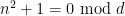
For any positive integer , let denote the number of solutions to the Diophantine equation

where are positive integers (we allow repetitions, and do not require the to be increasing). The Erdös-Straus conjecture asserts that for all . By dividing through by any positive integer we see that , so it suffices to verify this conjecture for primes , i.e. to solve the Diophantine equation

for each prime . As the case is easily solved, we may of course restrict attention to odd primes.

This conjecture remains open, although there is a reasonable amount of evidence towards its truth. For instance, it was shown by Vaughan that for any large , the number of exceptions to the Erdös-Straus conjecture with is at most for some absolute constant . The Erdös-Straus conjecture is also verified in several congruence classes of primes; for instance, from the identity

we see that the conjecture holds when . Further identities of this type can be used to resolve the conjecture unless is a quadratic residue mod , which leaves only six residue classes in that modulus to check (namely, , and ). However, there is a significant obstruction to eliminating the quadratic residue classes, as we will discuss later.

By combining these reductions with extensive numerical calculations, the Erdös-Straus conjecture was verified for all by Swett.

One approach to solving Diophantine equations such as (1) is to use methods of analytic number theory, such as the circle method, to obtain asymptotics (or at least lower bounds) for the number of solutions (or some proxy for this number); if one obtains a lower bound which is nontrivial for every , one has solved the problem. (One can alternatively view such methods as a variant of the probabilistic method; in this interpretation, one chooses the unknowns according to some suitable probability distribution and then tries to show that the probability of solving the equation is positive.) Such techniques can be effective for instance for certain instances of the Waring problem. However, as a general rule, these methods only work when there are a lot of solutions, and specifically when the number of solutions grows at a polynomial rate with the parameter .

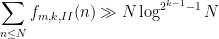
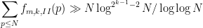
The first main result of my paper is that the number of solutions is essentially logarithmic in nature, thus providing a serious obstruction to solution by analytic methods, as there is almost no margin of error available. More precisely, I show that for almost all primes (i.e. in a subset of primes of relative density ), one has , or more precisely that

Readers familiar with analytic number theory will recognise the right-hand side from the divisor bound, which indeed plays a role in the proof.

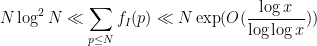
Actually, there are more precise estimates which suggest (though do not quite prove) that the mean value of is comparable to . To state these results properly, I need some more notation. It is not difficult to show that if is an odd prime and obey (1), then at least one, but not all, of the must be a multiple of . Thus we can split , where is the number of solutions to (1) where exactly of the are divisible by . The sharpest estimates I can prove are then

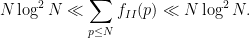
Theorem 1 For all sufficiently large , one has

and

Since the number of primes less than is comparable to by the prime number theorem, this shows that the mean value of in this range is between and , and the mean value of is between and , which gives the previous result as a corollary (thanks to a Markov inequality argument). A naive Poisson process heuristic then suggests that each prime has a “probability” of having a solution to (1), which by the Borel-Cantelli lemma heuristically suggests that there are only finitely many for which (1) fails. Of course, this is far from a rigorous proof (though the result of Vaughan mentioned earlier, which is based on the large sieve, can be viewed as a partial formalisation of the argument).

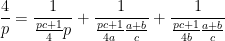
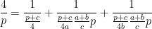
The first step in obtaining these results is an elementary description of in terms of some divisibility constraints. More precisely, we have

Lemma 2 Let be an odd prime. Then is equal to three times the number of triples of positive integers, with coprime, dividing , and dividing . Similarly, is equal to three times the number of triples of positive integers, with coprime, dividing , and dividing .

One direction of this lemma is very easy: if divides and divides then the identity

and its cyclic permutations give three contributions to , and similarly if divides instead then the identity

and its cyclic permutations give three contributions to . Conversely, some elementary number theory can be used to show that all solutions contributing to either or are of these forms. (Similar criteria have been used in prior literature, for instance in the previously mentioned paper of Vaughan.)

This lemma, incidentally, provides a way to quickly generate a large number of congruences of primes for which the Erdös-Straus conjecture can be verified. Indeed, from the above lemma we see that if are coprime and is any odd factor of (and hence coprime to ), then the Erdös-Straus conjecture is true whenever or . For instance,

• Taking , we see that the conjecture holds whenever (leaving only those primes );
• Taking we see that the conjecture holds whenever (leaving only those primes );
• Taking , we see that the conjecture holds whenever ((leaving only those primes );
• Taking , we see that the conjecture holds whenever (leaving only those primes );
• Taking , we see that the conjecture holds whenever ; taking instead , we see that the conjecture holds whenever . (This leaves only the primes that are equal to one of the six quadratic residues , an observation first made by Mordell.)
• etc.

If we let (resp. ) be the number of triples with coprime, dividing , and congruent to (resp. ) mod , the above lemma tells us that for all odd primes , so it suffices to show that are non-zero for all . One might hope that there are enough congruence relations provided by the previous observation to obtain a covering system of congruences which would resolve the conjecture. Unfortunately, as was also observed by Mordell, an application of the quadratic reciprocity law shows that these congruence relations cannot eliminate quadratic residues, only quadratic non-residues. More precisely, one can show that if are as above (restricting to the case , which contains all the unsolved cases of the conjecture) and is the largest odd factor of , then the Jacobi symbols and are always equal to . One consequence of this is that whenever is an odd perfect square. This makes it quite hard to resolve the conjecture for odd primes which resemble a perfect square in that they lie in quadratic residue classes to small moduli (and, from Dirichlet’s theorem on primes in arithmetic progressions, one can find many primes of this type). The same argument also shows that for an odd prime , there are no solutions to

in which one or two of the are divisible by , with the other denominators being coprime to . (Of course, one can still get representations of by starting with a representation of and dividing by , but such representations are is not of the above form.) This shows that any attempt to establish the Erdös-Straus conjecture by manually constructing as a function of must involve a technique which breaks down if is replaced by (for instance, this rules out any approach based on using polynomial combinations of and dividing into cases based on residue classes of in small moduli). Part of the problem here is that we do not have good bounds that prevent a prime from “spoofing” a perfect square to all small moduli (say, to all moduli less than a small power of ); this problem is closely related (via quadratic reciprocity) to Vinogradov’s conjecture on the least quadratic nonresidue, discussed in this previous blog post.

It remains to control the sums for . The lower bounds are relatively routine to establish, arising from counting the contribution of those that are somewhat small (e.g. less than ), and use only standard asymptotics of arithmetic functions and the Bombieri-Vinogradov inequality (to handle the restriction of the summation to primes). To obtain (nearly) matching upper bounds, one needs to prevent from getting too large. In the case of , the fact that divides and divides soon leads one to the bounds , at which point one can count primes in residue classes modulo with reasonable efficiency via the Brun-Titchmarsh inequality. This inequality unfortunately introduces a factor of , which we were only able to handle by bounding it crudely by , leading to the double logarithmic loss in the sum.

For , these arguments do not give good bounds, because it is possible for to be much larger than , and one can no longer easily count solutions to . However, an elementary change of variables resolves this problem. It turns out that if one lets be the positive integers

then one can convert the triple to a triple obeying the constraints

Conversely, every such triple determines by the formulae

The point is that this transformation now places in a residue class modulo rather than , and with , this allows one to count the number of solutions reasonably efficiently. The main loss now comes from counting the number of divisors of ; in particular, one becomes interested in estimating sums such as

where are less than and is the number of divisors of . In principle, because behaves like on the average (as can be seen from the Dirichlet hyperbola method), we expect this sum to be of order , but I was unable to show this, instead using the far cruder divisor bound

to obtain an upper bound of . Any improvement upon this bound would lead to a corresponding improvement in the upper bound for . While improvement is possible in some ranges (particularly when is large) using various bounds on Kloosterman-type exponential sums, I was not able to adequately control these sums when was fairly small (e.g. polylogarithmic size in ), as one could no longer extract much of an averaging effect from the summation in that case. Part of the difficulty is that in that case one must somehow exploit the fact that is irreducible as a polynomial in for any fixed , otherwise there will be too many divisors.

Polynomial bounds via nonstandard analysis

I have blogged several times in the past about nonstandard analysis, which among other things is useful in allowing one to import tools from infinitary (or qualitative) mathematics in order to establish results in finitary (or quantitative) mathematics. One drawback, though, to using nonstandard analysis methods is that the bounds one obtains by such methods are usually ineffective: in particular, the conclusions of a nonstandard analysis argument may involve an unspecified constant that is known to be finite but for which no explicit bound is obviously available. (In many cases, a bound can eventually be worked out by performing proof mining on the argument, and in particular by carefully unpacking the proofs of all the various results from infinitary mathematics that were used in the argument, as opposed to simply using them as “black boxes”, but this is a time-consuming task and the bounds that one eventually obtains tend to be quite poor (e.g. tower exponential or Ackermann type bounds are not uncommon).)

Because of this fact, it would seem that quantitative bounds, such as polynomial type bounds that show that one quantity is controlled in a polynomial fashion by another quantity , are not easily obtainable through the ineffective methods of nonstandard analysis. Actually, this is not the case; as I will demonstrate by an example below, nonstandard analysis can certainly yield polynomial type bounds. The catch is that the exponent in such bounds will be ineffective; but nevertheless such bounds are still good enough for many applications.

Let us now illustrate this by reproving a lemma from this paper of Mei-Chu Chang (Lemma 2.14, to be precise), which was recently pointed out to me by Van Vu. Chang’s paper is focused primarily on the sum-product problem, but she uses a quantitative lemma from algebraic geometry which is of independent interest. To motivate the lemma, let us first establish a qualitative version:

Lemma 1 (Qualitative solvability) Let be a finite number of polynomials in several variables with rational coefficients. If there is a complex solution to the simultaneous system of equations

then there also exists a solution whose coefficients are algebraic numbers (i.e. they lie in the algebraic closure of the rationals).

Proof: Suppose there was no solution to over . Applying Hilbert’s nullstellensatz (which is available as is algebraically closed), we conclude the existence of some polynomials (with coefficients in ) such that

as polynomials. In particular, we have

for all . This shows that there is no solution to over , as required.

Remark 1 Observe that in the above argument, one could replace and by any other pair of fields, with the latter containing the algebraic closure of the former, and still obtain the same result.

The above lemma asserts that if a system of rational equations is solvable at all, then it is solvable with some algebraic solution. But it gives no bound on the complexity of that solution in terms of the complexity of the original equation. Chang’s lemma provides such a bound. If is an integer, let us say that an algebraic number has height at most if its minimal polynomial (after clearing denominators) consists of integers of magnitude at most .

Lemma 2 (Quantitative solvability) Let be a finite number of polynomials of degree at most with rational coefficients, each of height at most . If there is a complex solution to the simultaneous system of equations

then there also exists a solution whose coefficients are algebraic numbers of degree at most and height at most , where depends only on , and .

Chang proves this lemma by essentially establishing a quantitative version of the nullstellensatz, via elementary elimination theory (somewhat similar, actually, to the approach I took to the nullstellensatz in my own blog post). She also notes that one could also establish the result through the machinery of Gröbner bases. In each of these arguments, it was not possible to use Lemma 1 (or the closely related nullstellensatz) as a black box; one actually had to unpack one of the proofs of that lemma or nullstellensatz to get the polynomial bound. However, using nonstandard analysis, it is possible to get such polynomial bounds (albeit with an ineffective value of the constant ) directly from Lemma 1 (or more precisely, the generalisation in Remark 1) without having to inspect the proof, and instead simply using it as a black box, thus providing a “soft” proof of Lemma 2 that is an alternative to the “hard” proofs mentioned above.

Here’s how the proof works. Informally, the idea is that Lemma 2 should follow from Lemma 1 after replacing the field of rationals with “the field of rationals of polynomially bounded height”. Unfortunately, the latter object does not really make sense as a field in standard analysis; nevertheless, it is a perfectly sensible object in nonstandard analysis, and this allows the above informal argument to be made rigorous.

We turn to the details. As is common whenever one uses nonstandard analysis to prove finitary results, we use a “compactness and contradiction” argument (or more precisely, an “ultralimit and contradiction” argument). Suppose for contradiction that Lemma 2 failed. Carefully negating the quantifiers (and using the axiom of choice), we conclude that there exists such that for each natural number , there is a positive integer and a family of polynomials of degree at most and rational coefficients of height at most , such that there exist at least one complex solution to

but such that there does not exist any such solution whose coefficients are algebraic numbers of degree at most and height at most .

Now we take ultralimits (see e.g. this previous blog post of a quick review of ultralimit analysis, which we will assume knowledge of in the argument that follows). Let be a non-principal ultrafilter. For each , the ultralimit

of the (standard) polynomials is a nonstandard polynomial of degree at most , whose coefficients now lie in the nonstandard rationals . Actually, due to the height restriction, we can say more. Let be the ultralimit of the , this is a nonstandard natural number (which will almost certainly be unbounded, but we will not need to use this). Let us say that a nonstandard integer is of polynomial size if we have for some standard natural number , and say that a nonstandard rational number is of polynomial height if , are of polynomial size. Let be the collection of all nonstandard rationals of polynomial height. (In the language of nonstandard analysis, is an external set rather than an internal one, because it is not itself an ultraproduct of standard sets; but this will not be relevant for the argument that follows.) It is easy to see that is a field, basically because the sum or product of two integers of polynomial size, remains of polynomial size. By construction, it is clear that the coefficients of are nonstandard rationals of polynomial height, and thus are defined over .

Meanwhile, if we let be the ultralimit of the solutions in (1), we have

thus are solvable in . Applying Lemma 1 (or more precisely, the generalisation in Remark 1), we see that are also solvable in . (Note that as is algebraically closed, is also (by Los’s theorem), and so contains .) Thus, there exists with

As lies in , we can write as an ultralimit of standard complex vectors . By construction, the coefficients of each obey a non-trivial polynomial equation of degree at most and whose coefficients are nonstandard integers of magnitude at most , for some standard natural number . Undoing the ultralimit, we conclude that for sufficiently close to , the coefficients of obey a non-trivial polynomial equation of degree at most whose coefficients are standard integers of magnitude at most . In particular, these coefficients have height at most . Also, we have

But for larger than , this contradicts the construction of the , and the claim follows. (Note that as is non-principal, any neighbourhood of in will contain arbitrarily large natural numbers.)

Remark 2 The same argument actually gives a slightly stronger version of Lemma 2, namely that the integer coefficients used to define the algebraic solution can be taken to be polynomials in the coefficients of , with degree and coefficients bounded by .

Compactness and contradiction

I recently finished the first draft of the last of my books based on my 2010 blog posts (and also my Google buzzes), entitled “Compactness and contradiction“.    The PDF of this draft is available here.  This is a somewhat assorted (and lightly edited) collection of posts (and buzzes), though concentrating in the areas of analysis (both standard and nonstandard), logic, and group theory.   As always, comments and corrections are welcome.