
You are currently browsing the category archive for the ‘255B – incompressible Euler equations’ category.
We consider the incompressible Euler equations on the (Eulerian) torus 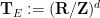


As noted previously, the kinetic energy
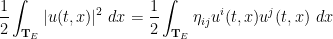
 is the Euclidean metric. Indeed, if one assumes that
  are continuously differentiable in both space and time on
 ![{[0,T] \times \mathbf{T}}](https://s0.wp.com/latex.php?latex=%7B%5B0%2CT%5D+%5Ctimes+%5Cmathbf%7BT%7D%7D&bg=ffffff&fg=000000&s=0&c=20201002) , then one can multiply the equation (1) by
, then one can multiply the equation (1) by  and contract against
  to obtain
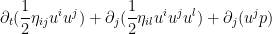
![{[0,T] \times \mathbf{T}_E}](https://s0.wp.com/latex.php?latex=%7B%5B0%2CT%5D+%5Ctimes+%5Cmathbf%7BT%7D_E%7D&bg=ffffff&fg=000000&s=0&c=20201002) and uses Stokes’ theorem, one obtains the required energy conservation law
and uses Stokes’ theorem, one obtains the required energy conservation law 
 is not a test function and so one cannot immediately integrate (1) against . And indeed, as we shall soon see, it is now known that once the regularity of
  is low enough, energy can “escape to frequency infinity”, leading to failure of the energy conservation law, a phenomenon known in physics as anomalous energy dissipation.
But what is the precise level of regularity needed in order to for this anomalous energy dissipation to occur? To make this question precise, we need a quantitative notion of regularity. One such measure is given by the Hölder space 


 lies between the space
  of continuous functions and the space
  of continuously differentiable functions, and informally describes a space of functions that is “
 times differentiable” in some sense. The above derivation of the energy conservation law involved the integral
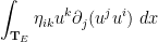
 once
once  . More precisely, one can make
Conjecture 1 (Onsager’s conjecture) Let, and let
.
- (i) If
to the Euler equations (in the Leray form
) obeys the energy conservation law (3).
- (ii) If
, then there exist weak solutions
This conjecture was originally arrived at by Onsager by a somewhat different heuristic derivation; see Remark 7. The numerology is also compatible with that arising from the Kolmogorov theory of turbulence (discussed in this previous post), but we will not discuss this interesting connection further here.
The positive part (i) of Onsager conjecture was established by Constantin, E, and Titi, building upon earlier partial results by Eyink; the proof is a relatively straightforward application of Littlewood-Paley theory, and they were also able to work in larger function spaces than 


In these notes we will first establish (i), then discuss the convex integration method in the original context of the Nash-Kuiper embedding theorem. Before tackling the Onsager conjecture (ii) directly, we discuss a related construction of high-dimensional weak solutions in the Sobolev space 


We thank Phil Isett for some comments and corrections.
These lecture notes are a continuation of the 254A lecture notes from the previous quarter.
We consider the Euler equations for incompressible fluid flow on a Euclidean space 


In Eulerian coordinates, the Euler equations read


where 


We will refer to the coordinates
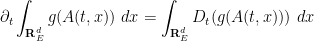
In view of this, it is natural to ask whether there is an alternate way to formulate the continuum limit of incompressible inviscid fluids, by using a continuous version 


Given a smooth and bounded velocity field 

in view of (2), this describes the trajectory (in 
for 

Despite the popularity of the initial condition (4), we will try to keep conceptually separate the Eulerian space 
Exercise 1 Let
- If
is a smooth map, show that there exists a unique smooth trajectory map
for all
- Show that if
is a diffeomorphism and
is also a diffeomorphism.
Remark 2 The first of the Euler equations (1) can now be written in the form
which can be viewed as a continuous limit of Newton’s first law
.
Call a diffeomorphism 
for all 


for all 


The divergence-free condition 

Lemma 3 Let
is volume-preserving for all
Proof: Since 

for all
for all
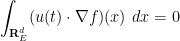
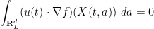
which by integration by parts gives

for all
To prove the converse implication, it is convenient to introduce the labels map 

for all 

where 
acting on functions on

for any test function 

and hence

for any 
Thus 

Exercise 4 Let
be a continuously differentiable map from the time interval
to the general linear group
of invertible
and use this and (6) to give an alternate proof of Lemma 3 that does not involve any integration in space.

Remark 5 One can view the use of Lagrangian coordinates as an extension of the method of characteristics. Indeed, from the chain rule we see that for any smooth function
of Eulerian spacetime, one has
and hence any transport equation that in Eulerian coordinates takes the form
for smooth functions
of Eulerian spacetime is equivalent to the ODE
where
are the smooth functions of Lagrangian spacetime defined by


In this set of notes we recall some basic differential geometry notation, particularly with regards to pullbacks and Lie derivatives of differential forms and other tensor fields on manifolds such as
Remark 6 One can also write the Navier-Stokes equations in Lagrangian coordinates, but the equations are not expressed in a favourable form in these coordinates, as the Laplacian
appearing in the viscosity term becomes replaced with a time-varying Laplace-Beltrami operator. As such, we will not discuss the Lagrangian coordinate formulation of Navier-Stokes here.

Recent Comments