I’ve just uploaded to the arXiv my paper “Embedding the Heisenberg group into a bounded dimensional Euclidean space with optimal distortion“, submitted to Revista Matematica Iberoamericana. This paper concerns the extent to which one can accurately embed the metric structure of the Heisenberg group
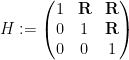
into Euclidean space, which we can write as ![{\{ [x,y,z]: x,y,z \in {\bf R} \}}](https://s0.wp.com/latex.php?latex=%7B%5C%7B+%5Bx%2Cy%2Cz%5D%3A+x%2Cy%2Cz+%5Cin+%7B%5Cbf+R%7D+%5C%7D%7D&bg=ffffff&fg=000000&s=0&c=20201002) with the notation
with the notation
![\displaystyle [x,y,z] := \begin{pmatrix} 1 & x & z \\ 0 & 1 & y \\ 0 & 0 & 1 \end{pmatrix}.](https://s0.wp.com/latex.php?latex=%5Cdisplaystyle+%5Bx%2Cy%2Cz%5D+%3A%3D+%5Cbegin%7Bpmatrix%7D+1+%26+x+%26+z+%5C%5C+0+%26+1+%26+y+%5C%5C+0+%26+0+%26+1+%5Cend%7Bpmatrix%7D.&bg=ffffff&fg=000000&s=0&c=20201002)
Here we give  the right-invariant Carnot-Carathéodory metric
  coming from the right-invariant vector fields
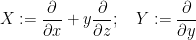
but not from the commutator vector field
![\displaystyle Z := [Y,X] = \frac{\partial}{\partial z}.](https://s0.wp.com/latex.php?latex=%5Cdisplaystyle+Z+%3A%3D+%5BY%2CX%5D+%3D+%5Cfrac%7B%5Cpartial%7D%7B%5Cpartial+z%7D.&bg=ffffff&fg=000000&s=0&c=20201002)
This gives the geometry of a Carnot group. As observed by Semmes, it follows from the Carnot group differentiation theory of Pansu that there is no bilipschitz map from  to any Euclidean space
  or even to
  , since such a map must be differentiable almost everywhere in the sense of Carnot groups, which in particular shows that the derivative map annihilate
  almost everywhere, which is incompatible with being bilipschitz.
On the other hand, if one snowflakes the Heisenberg group by replacing the metric with  for some
  , then it follows from the general theory of Assouad on embedding snowflaked metrics of doubling spaces that
  may be embedded in a bilipschitz fashion into , or even to
  for some
  depending on
  .
.
Of course, the distortion of this bilipschitz embedding must degenerate in the limit  . From the work of Austin-Naor-Tessera and Naor-Neiman it follows that may be embedded into with a distortion of
  , but no better. The Naor-Neiman paper also embeds into a finite-dimensional space with
  independent of , but at the cost of worsening the distortion to
  . They then posed the question of whether this worsening of the distortion is necessary.
The main result of this paper answers this question in the negative:
Theorem 1 There exists an absolute constant such that may be embedded into in a bilipschitz fashion with distortion  for any
  .
.
To motivate the proof of this theorem, let us first present a bilipschitz map  from the snowflaked line
  (with
(with  being the usual metric on
  ) into complex Hilbert space
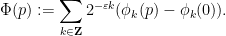
  . The map is given explicitly as a Weierstrass type function
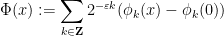
where for each  ,
,  is the function
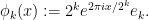
and  are an orthonormal basis for . The subtracting of the constant
  is purely in order to make the sum convergent as
  . If
. If  are such that
  for some integer
  , one can easily check the bounds

with the lower bound

at which point one finds that

as desired.
The key here was that each function  oscillated at a different spatial scale
  , and the functions were all orthogonal to each other (so that the upper bound involved a factor of
  rather than
  ). One can replicate this example for the Heisenberg group without much difficulty. Indeed, if we let
 ![{\Gamma := \{ [a,b,c]: a,b,c \in {\bf Z} \}}](https://s0.wp.com/latex.php?latex=%7B%5CGamma+%3A%3D+%5C%7B+%5Ba%2Cb%2Cc%5D%3A+a%2Cb%2Cc+%5Cin+%7B%5Cbf+Z%7D+%5C%7D%7D&bg=ffffff&fg=000000&s=0&c=20201002) be the discrete Heisenberg group, then the nilmanifold
be the discrete Heisenberg group, then the nilmanifold  is a three-dimensional smooth compact manifold; thus, by the Whitney embedding theorem, it smoothly embeds into
  . This gives a smooth immersion
  which is
  -automorphic in the sense that
  for all
  and
and  . If one then defines
  to be the function

where  is the scaling map
![\displaystyle \delta_\lambda([x,y,z]) := [\lambda x, \lambda y, \lambda^2 z],](https://s0.wp.com/latex.php?latex=%5Cdisplaystyle+%5Cdelta_%5Clambda%28%5Bx%2Cy%2Cz%5D%29+%3A%3D+%5B%5Clambda+x%2C+%5Clambda+y%2C+%5Clambda%5E2+z%5D%2C&bg=ffffff&fg=000000&s=0&c=20201002)
then one can repeat the previous arguments to obtain the required bilipschitz bounds

for the function
To adapt this construction to bounded dimension, the main obstruction was the requirement that the took values in orthogonal subspaces. But if one works things out carefully, it is enough to require the weaker orthogonality requirement
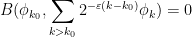
for all  , where
  is the bilinear form

One can then try to construct the  for bounded dimension by an iterative argument. After some standard reductions, the problem becomes this (roughly speaking): given a smooth, slowly varying function
  whose derivatives obey certain quantitative upper and lower bounds, construct a smooth oscillating function
  , whose derivatives also obey certain quantitative upper and lower bounds, which obey the equation
We view this as an underdetermined system of differential equations for  (two equations in unknowns; after some reductions, our can be taken to be the explicit value
  ). The trivial solution
  to this equation will be inadmissible for our purposes due to the lower bounds we will require on (in order to obtain the quantitative immersion property mentioned previously, as well as for a stronger “freeness” property that is needed to close the iteration). Because this construction will need to be iterated, it will be essential that the regularity control on is the same as that on
  ; one cannot afford to “lose derivatives” when passing from to .
This problem has some formal similarities with the isometric embedding problem (discussed for instance in this previous post), which can be viewed as the problem of solving an equation of the form  , where
  is a Riemannian manifold and
  is the bilinear form
The isometric embedding problem also has the key obstacle that naive attempts to solve the equation  iteratively can lead to an undesirable “loss of derivatives” that prevents one from iterating indefinitely. This obstacle was famously resolved by the Nash-Moser iteration scheme in which one alternates between perturbatively adjusting an approximate solution to improve the residual error term, and mollifying the resulting perturbation to counteract the loss of derivatives. The current equation (1) differs in some key respects from the isometric embedding equation , in particular being linear in the unknown field rather than quadratic; nevertheless the key obstacle is the same, namely that naive attempts to solve either equation lose derivatives. Our approach to solving (1) was inspired by the Nash-Moser scheme; in retrospect, I also found similarities with Uchiyama’s constructive proof of the Fefferman-Stein decomposition theorem, discussed in this previous post (and in this recent one).
To motivate this iteration, we first express  using the product rule in a form that does not place derivatives directly on the unknown :

This reveals that one can construct solutions to (1) by solving the system of equations

for  . Because this system is zeroth order in , this can easily be done by linear algebra (even in the presence of a forcing term
  ) if one imposes a “freeness” condition (analogous to the notion of a free embedding in the isometric embedding problem) that
  are linearly independent at each point
  , which (together with some other technical conditions of a similar nature) one then adds to the list of upper and lower bounds required on (with a related bound then imposed on , in order to close the iteration). However, as mentioned previously, there is a “loss of derivatives” problem with this construction: due to the presence of the differential operators
  in (3), a solution constructed by this method can only be expected to have two degrees less regularity than at best, which makes this construction unsuitable for iteration.
To get around this obstacle (which also prominently appears when solving (linearisations of) the isometric embedding equation ), we instead first construct a smooth, low-frequency solution  to a low-frequency equation

where  is a mollification of (of Littlewood-Paley type) applied at a small spatial scale
  for some
  , and then gradually relax the frequency cutoff
  to deform this low frequency solution
  to a solution of the actual equation (1).
We will construct the low-frequency solution rather explicitly, using the Whitney embedding theorem to construct an initial oscillating map  into a very low dimensional space , composing it with a Veronese type embedding into a slightly larger dimensional space
  to obtain a required “freeness” property, and then composing further with a slowly varying isometry
  depending on and constructed by a quantitative topological lemma (relying ultimately on the vanishing of the first few homotopy groups of high-dimensional spheres), in order to obtain the required orthogonality (4). (This sort of “quantitative null-homotopy” was first proposed by Gromov, with some recent progress on optimal bounds by Chambers-Manin-Weinberger and by Chambers-Dotterer-Manin-Weinberger, but we will not need these more advanced results here, as one can rely on the classical qualitative vanishing
  for
for  together with a compactness argument to obtain (ineffective) quantitative bounds, which suffice for this application).
To perform the deformation of into , we must solve what is essentially the linearised equation

of (1) when , (viewed as low frequency functions) are both being deformed at some rates  (which should be viewed as high frequency functions). To avoid losing derivatives, the magnitude of the deformation
  in should not be significantly greater than the magnitude of the deformation
  in , when measured in the same function space norms.
As before, if one directly solves the difference equation (5) using a naive application of (2) with  treated as a forcing term, one will lose at least one derivative of regularity when passing from to . However, observe that (2) (and the symmetry
  ) can be used to obtain the identity

and then one can solve (5) by solving the system of equations
for  . The key point here is that this system is zeroth order in both and , so one can solve this system without losing any derivatives when passing from to ; compare this situation with that of the superficially similar system
that one would obtain from naively linearising (3) without exploiting the symmetry of  . There is still however one residual “loss of derivatives” problem arising from the presence of a differential operator on the term, which prevents one from directly evolving this iteration scheme in time without losing regularity in . It is here that we borrow the final key idea of the Nash-Moser scheme, which is to replace by a mollified version
  of itself (where the projection
  depends on the time parameter). This creates an error term in (5), but it turns out that this error term is quite small and smooth (being a “high-high paraproduct” of
  and
and  , it ends up being far more regular than either or , even with the presence of the derivatives) and can be iterated away provided that the initial frequency cutoff is large and the function has a fairly high (but finite) amount of regularity (we will eventually use the Hölder space
  on the Heisenberg group to measure this).


Recent Comments