“Introduction to measure theory” now published

My graduate text on measure theory (based on these lecture notes) is now published by the AMS as part of the Graduate Studies in Mathematics series.  (See also my own blog page for this book, which among other things contains a draft copy of the book in PDF format.)

245A, Notes 6: Outer measures, pre-measures, and product measures

In this course so far, we have focused primarily on one specific example of a countably additive measure, namely Lebesgue measure. This measure was constructed from a more primitive concept of Lebesgue outer measure, which in turn was constructed from the even more primitive concept of elementary measure.
It turns out that both of these constructions can be abstracted. In this set of notes, we will give the Carathéodory lemma, which constructs a countably additive measure from any abstract outer measure; this generalises the construction of Lebesgue measure from Lebesgue outer measure. One can in turn construct outer measures from another concept known as a pre-measure, of which elementary measure is a typical example.
With these tools, one can start constructing many more measures, such as Lebesgue-Stieltjes measures, product measures, and Hausdorff measures. With a little more effort, one can also establish the Kolmogorov extension theorem, which allows one to construct a variety of measures on infinite-dimensional spaces, and is of particular importance in the foundations of probability theory, as it allows one to set up probability spaces associated to both discrete and continuous random processes, even if they have infinite length.
The most important result about product measure, beyond the fact that it exists, is that one can use it to evaluate iterated integrals, and to interchange their order, provided that the integrand is either unsigned or absolutely integrable. This fact is known as the Fubini-Tonelli theorem, and is an absolutely indispensable tool for computing integrals, and for deducing higher-dimensional results from lower-dimensional ones.
We remark that these notes omit a very important way to construct measures, namely the Riesz representation theorem, but we will defer discussion of this theorem to 245B.
This is the final set of notes in this sequence. If time permits, the course will then begin covering the 245B notes, starting with the material on signed measures and the Radon-Nikodym-Lebesgue theorem.

245A: Problem solving strategies

This is going to be a somewhat experimental post. In class, I mentioned that when solving the type of homework problems encountered in a graduate real analysis course, there are really only about a dozen or so basic tricks and techniques that are used over and over again. But I had not thought to actually try to make these tricks explicit, so I am going to try to compile here a list of some of these techniques here. But this list is going to be far from exhaustive; perhaps if other recent students of real analysis would like to share their own methods, then I encourage you to do so in the comments (even – or especially – if the techniques are somewhat vague and general in nature).

(See also the Tricki for some general mathematical problem solving tips.  Once this page matures somewhat, I might migrate it to the Tricki.)

Note: the tricks occur here in no particular order, reflecting the stream-of-consciousness way in which they were arrived at.  Indeed, this list will be extended on occasion whenever I find another trick that can be added to this list.

245A, Notes 5: Differentiation theorems

Let be a compact interval of positive length (thus ). Recall that a function is said to be differentiable at a point if the limit

exists. In that case, we call the strong derivative, classical derivative, or just derivative for short, of at . We say that is everywhere differentiable, or differentiable for short, if it is differentiable at all points , and differentiable almost everywhere if it is differentiable at almost every point . If is differentiable everywhere and its derivative is continuous, then we say that is continuously differentiable.

Remark 1 Much later in this sequence, when we cover the theory of distributions, we will see the notion of a weak derivative or distributional derivative, which can be applied to a much rougher class of functions and is in many ways more suitable than the classical derivative for doing “Lebesgue” type analysis (i.e. analysis centred around the Lebesgue integral, and in particular allowing functions to be uncontrolled, infinite, or even undefined on sets of measure zero). However, for now we will stick with the classical approach to differentiation.

Exercise 2 If is everywhere differentiable, show that is continuous and is measurable. If is almost everywhere differentiable, show that the (almost everywhere defined) function is measurable (i.e. it is equal to an everywhere defined measurable function on outside of a null set), but give an example to demonstrate that need not be continuous.

Exercise 3 Give an example of a function which is everywhere differentiable, but not continuously differentiable. (Hint: choose an that vanishes quickly at some point, say at the origin , but which also oscillates rapidly near that point.)

In single-variable calculus, the operations of integration and differentiation are connected by a number of basic theorems, starting with Rolle’s theorem.

Theorem 4 (Rolle’s theorem) Let be a compact interval of positive length, and let be a differentiable function such that . Then there exists such that .

Proof: By subtracting a constant from (which does not affect differentiability or the derivative) we may assume that . If is identically zero then the claim is trivial, so assume that is non-zero somewhere. By replacing with if necessary, we may assume that is positive somewhere, thus . On the other hand, as is continuous and is compact, must attain its maximum somewhere, thus there exists such that for all . Then must be positive and so cannot equal either or , and thus must lie in the interior. From the right limit of (1) we see that , while from the left limit we have . Thus and the claim follows.

Remark 5 Observe that the same proof also works if is only differentiable in the interior of the interval , so long as it is continuous all the way up to the boundary of .

Exercise 6 Give an example to show that Rolle’s theorem can fail if is merely assumed to be almost everywhere differentiable, even if one adds the additional hypothesis that is continuous. This example illustrates that everywhere differentiability is a significantly stronger property than almost everywhere differentiability. We will see further evidence of this fact later in these notes; there are many theorems that assert in their conclusion that a function is almost everywhere differentiable, but few that manage to conclude everywhere differentiability.

Remark 7 It is important to note that Rolle’s theorem only works in the real scalar case when is real-valued, as it relies heavily on the least upper bound property for the domain . If, for instance, we consider complex-valued scalar functions , then the theorem can fail; for instance, the function defined by vanishes at both endpoints and is differentiable, but its derivative is never zero. (Rolle’s theorem does imply that the real and imaginary parts of the derivative both vanish somewhere, but the problem is that they don’t simultaneously vanish at the same point.) Similar remarks to functions taking values in a finite-dimensional vector space, such as .

One can easily amplify Rolle’s theorem to the mean value theorem:

Corollary 8 (Mean value theorem) Let be a compact interval of positive length, and let be a differentiable function. Then there exists such that .

Proof: Apply Rolle’s theorem to the function .

Remark 9 As Rolle’s theorem is only applicable to real scalar-valued functions, the more general mean value theorem is also only applicable to such functions.

Exercise 10 (Uniqueness of antiderivatives up to constants) Let be a compact interval of positive length, and let and be differentiable functions. Show that for every if and only if for some constant and all .

We can use the mean value theorem to deduce one of the fundamental theorems of calculus:

Theorem 11 (Second fundamental theorem of calculus) Let be a differentiable function, such that is Riemann integrable. Then the Riemann integral of is equal to . In particular, we have whenever is continuously differentiable.

Proof: Let . By the definition of Riemann integrability, there exists a finite partition such that

for every choice of .
Fix this partition. From the mean value theorem, for each one can find such that

and thus by telescoping series

Since was arbitrary, the claim follows.

Remark 12 Even though the mean value theorem only holds for real scalar functions, the fundamental theorem of calculus holds for complex or vector-valued functions, as one can simply apply that theorem to each component of that function separately.

Of course, we also have the other half of the fundamental theorem of calculus:

Theorem 13 (First fundamental theorem of calculus) Let be a compact interval of positive length. Let be a continuous function, and let be the indefinite integral . Then is differentiable on , with derivative for all . In particular, is continuously differentiable.

Proof: It suffices to show that

for all , and

for all . After a change of variables, we can write

for any and any sufficiently small , or any and any sufficiently small . As is continuous, the function converges uniformly to on as (keeping fixed). As the interval is bounded, thus converges to , and the claim follows.

Corollary 14 (Differentiation theorem for continuous functions) Let be a continuous function on a compact interval. Then we have

for all ,

for all , and thus

for all .

In these notes we explore the question of the extent to which these theorems continue to hold when the differentiability or integrability conditions on the various functions are relaxed. Among the results proven in these notes are

• The Lebesgue differentiation theorem, which roughly speaking asserts that Corollary 14 continues to hold for almost every if is merely absolutely integrable, rather than continuous;
• A number of differentiation theorems, which assert for instance that monotone, Lipschitz, or bounded variation functions in one dimension are almost everywhere differentiable; and
• The second fundamental theorem of calculus for absolutely continuous functions.

The material here is loosely based on Chapter 3 of Stein-Shakarchi.

Covering a non-closed interval by disjoint closed intervals

The following question came up in my 245A class today:

Is it possible to express a non-closed interval in the real line, such as [0,1), as a countable union of disjoint closed intervals?

I was not able to answer the question immediately, but by the end of the class some of the students had come up with an answer.  It is actually a nice little test of one’s basic knowledge of real analysis, so I am posing it here as well for anyone else who is interested.  Below the fold is the answer to the question (whited out; one has to highlight the text in order to read it).

245A, Notes 4: Modes of convergence

If one has a sequence of real numbers , it is unambiguous what it means for that sequence to converge to a limit : it means that for every , there exists an such that for all . Similarly for a sequence of complex numbers converging to a limit .

More generally, if one has a sequence of -dimensional vectors in a real vector space or complex vector space , it is also unambiguous what it means for that sequence to converge to a limit or ; it means that for every , there exists an such that for all . Here, the norm of a vector can be chosen to be the Euclidean norm , the supremum norm , or any other number of norms, but for the purposes of convergence, these norms are all equivalent; a sequence of vectors converges in the Euclidean norm if and only if it converges in the supremum norm, and similarly for any other two norms on the finite-dimensional space or .

If however one has a sequence of functions or on a common domain , and a putative limit or , there can now be many different ways in which the sequence may or may not converge to the limit . (One could also consider convergence of functions on different domains , but we will not discuss this issue at all here.) This is contrast with the situation with scalars or (which corresponds to the case when is a single point) or vectors (which corresponds to the case when is a finite set such as ). Once becomes infinite, the functions acquire an infinite number of degrees of freedom, and this allows them to approach in any number of inequivalent ways.

What different types of convergence are there? As an undergraduate, one learns of the following two basic modes of convergence:

1. We say that converges to pointwise if, for every , converges to . In other words, for every and , there exists (that depends on both and ) such that whenever .
2. We say that converges to uniformly if, for every , there exists such that for every , for every . The difference between uniform convergence and pointwise convergence is that with the former, the time at which must be permanently -close to is not permitted to depend on , but must instead be chosen uniformly in .

Uniform convergence implies pointwise convergence, but not conversely. A typical example: the functions defined by converge pointwise to the zero function , but not uniformly.

However, pointwise and uniform convergence are only two of dozens of many other modes of convergence that are of importance in analysis. We will not attempt to exhaustively enumerate these modes here (but see this Wikipedia page, and see also these 245B notes on strong and weak convergence). We will, however, discuss some of the modes of convergence that arise from measure theory, when the domain is equipped with the structure of a measure space , and the functions (and their limit ) are measurable with respect to this space. In this context, we have some additional modes of convergence:

1. We say that converges to pointwise almost everywhere if, for (-)almost everywhere , converges to .
2. We say that converges to uniformly almost everywhere, essentially uniformly, or in norm if, for every , there exists such that for every , for -almost every .
3. We say that converges to almost uniformly if, for every , there exists an exceptional set of measure such that converges uniformly to on the complement of .
4. We say that converges to in norm if the quantity converges to as .
5. We say that converges to in measure if, for every , the measures converge to zero as .

Observe that each of these five modes of convergence is unaffected if one modifies or on a set of measure zero. In contrast, the pointwise and uniform modes of convergence can be affected if one modifies or even on a single point.

Remark 1 In the context of probability theory, in which and are interpreted as random variables, convergence in norm is often referred to as convergence in mean, pointwise convergence almost everywhere is often referred to as almost sure convergence, and convergence in measure is often referred to as convergence in probability.

Exercise 2 (Linearity of convergence) Let be a measure space, let be sequences of measurable functions, and let be measurable functions.

1. Show that converges to along one of the above seven modes of convergence if and only if converges to along the same mode.
2. If converges to along one of the above seven modes of convergence, and converges to along the same mode, show that converges to along the same mode, and that converges to along the same mode for any .
3. (Squeeze test) If converges to along one of the above seven modes, and pointwise for each , show that converges to along the same mode.

We have some easy implications between modes:

Exercise 3 (Easy implications) Let be a measure space, and let and be measurable functions.

1. If converges to uniformly, then converges to pointwise.
2. If converges to uniformly, then converges to in norm. Conversely, if converges to in norm, then converges to uniformly outside of a null set (i.e. there exists a null set such that the restriction of to the complement of converges to the restriction of ).
3. If converges to in norm, then converges to almost uniformly.
4. If converges to almost uniformly, then converges to pointwise almost everywhere.
5. If converges to pointwise, then converges to pointwise almost everywhere.
6. If converges to in norm, then converges to in measure.
7. If converges to almost uniformly, then converges to in measure.

The reader is encouraged to draw a diagram that summarises the logical implications between the seven modes of convergence that the above exercise describes.

We give four key examples that distinguish between these modes, in the case when is the real line with Lebesgue measure. The first three of these examples already were introduced in the previous set of notes.

Example 4 (Escape to horizontal infinity) Let . Then converges to zero pointwise (and thus, pointwise almost everywhere), but not uniformly, in norm, almost uniformly, in norm, or in measure.

Example 5 (Escape to width infinity) Let . Then converges to zero uniformly (and thus, pointwise, pointwise almost everywhere, in norm, almost uniformly, and in measure), but not in norm.

Example 6 (Escape to vertical infinity) Let . Then converges to zero pointwise (and thus, pointwise almost everywhere) and almost uniformly (and hence in measure), but not uniformly, in norm, or in norm.

Example 7 (Typewriter sequence) Let be defined by the formula

whenever and . This is a sequence of indicator functions of intervals of decreasing length, marching across the unit interval over and over again. Then converges to zero in measure and in norm, but not pointwise almost everywhere (and hence also not pointwise, not almost uniformly, nor in norm, nor uniformly).

Remark 8 The norm of a measurable function is defined to the infimum of all the quantities that are essential upper bounds for in the sense that for almost every . Then converges to in norm if and only if as . The and norms are part of the larger family of norms, which we will study in more detail in 245B.

One particular advantage of convergence is that, in the case when the are absolutely integrable, it implies convergence of the integrals,

as one sees from the triangle inequality. Unfortunately, none of the other modes of convergence automatically imply this convergence of the integral, as the above examples show.
The purpose of these notes is to compare these modes of convergence with each other. Unfortunately, the relationship between these modes is not particularly simple; unlike the situation with pointwise and uniform convergence, one cannot simply rank these modes in a linear order from strongest to weakest. This is ultimately because the different modes react in different ways to the three “escape to infinity” scenarios described above, as well as to the “typewriter” behaviour when a single set is “overwritten” many times. On the other hand, if one imposes some additional assumptions to shut down one or more of these escape to infinity scenarios, such as a finite measure hypothesis or a uniform integrability hypothesis, then one can obtain some additional implications between the different modes.

245A, Notes 3: Integration on abstract measure spaces, and the convergence theorems

Thus far, we have only focused on measure and integration theory in the context of Euclidean spaces . Now, we will work in a more abstract and general setting, in which the Euclidean space is replaced by a more general space .

It turns out that in order to properly define measure and integration on a general space , it is not enough to just specify the set . One also needs to specify two additional pieces of data:

1. A collection of subsets of that one is allowed to measure; and
2. The measure one assigns to each measurable set .

For instance, Lebesgue measure theory covers the case when is a Euclidean space , is the collection of all Lebesgue measurable subsets of , and is the Lebesgue measure of .

The collection has to obey a number of axioms (e.g. being closed with respect to countable unions) that make it a -algebra, which is a stronger variant of the more well-known concept of a boolean algebra. Similarly, the measure has to obey a number of axioms (most notably, a countable additivity axiom) in order to obtain a measure and integration theory comparable to the Lebesgue theory on Euclidean spaces. When all these axioms are satisfied, the triple is known as a measure space. These play much the same role in abstract measure theory that metric spaces or topological spaces play in abstract point-set topology, or that vector spaces play in abstract linear algebra.

On any measure space, one can set up the unsigned and absolutely convergent integrals in almost exactly the same way as was done in the previous notes for the Lebesgue integral on Euclidean spaces, although the approximation theorems are largely unavailable at this level of generality due to the lack of such concepts as “elementary set” or “continuous function” for an abstract measure space. On the other hand, one does have the fundamental convergence theorems for the subject, namely Fatou’s lemma, the monotone convergence theorem and the dominated convergence theorem, and we present these results here.

One question that will not be addressed much in this current set of notes is how one actually constructs interesting examples of measures. We will discuss this issue more in later notes (although one of the most powerful tools for such constructions, namely the Riesz representation theorem, will not be covered until 245B).

245A, Notes 2: The Lebesgue integral

In the previous notes, we defined the Lebesgue measure of a Lebesgue measurable set , and set out the basic properties of this measure. In this set of notes, we use Lebesgue measure to define the Lebesgue integral

of functions . Just as not every set can be measured by Lebesgue measure, not every function can be integrated by the Lebesgue integral; the function will need to be Lebesgue measurable. Furthermore, the function will either need to be unsigned (taking values on ), or absolutely integrable.

To motivate the Lebesgue integral, let us first briefly review two simpler integration concepts. The first is that of an infinite summation

of a sequence of numbers , which can be viewed as a discrete analogue of the Lebesgue integral. Actually, there are two overlapping, but different, notions of summation that we wish to recall here. The first is that of the unsigned infinite sum, when the lie in the extended non-negative real axis . In this case, the infinite sum can be defined as the limit of the partial sums

 

or equivalently as a supremum of arbitrary finite partial sums:

 

The unsigned infinite sum always exists, but its value may be infinite, even when each term is individually finite (consider e.g. ).

The second notion of a summation is the absolutely summable infinite sum, in which the lie in the complex plane and obey the absolute summability condition

where the left-hand side is of course an unsigned infinite sum. When this occurs, one can show that the partial sums converge to a limit, and we can then define the infinite sum by the same formula (1) as in the unsigned case, though now the sum takes values in rather than . The absolute summability condition confers a number of useful properties that are not obeyed by sums that are merely conditionally convergent; most notably, the value of an absolutely convergent sum is unchanged if one rearranges the terms in the series in an arbitrary fashion. Note also that the absolutely summable infinite sums can be defined in terms of the unsigned infinite sums by taking advantage of the formulae

for complex absolutely summable , and

for real absolutely summable , where and are the (magnitudes of the) positive and negative parts of .

In an analogous spirit, we will first define an unsigned Lebesgue integral of (measurable) unsigned functions , and then use that to define the absolutely convergent Lebesgue integral of absolutely integrable functions . (In contrast to absolutely summable series, which cannot have any infinite terms, absolutely integrable functions will be allowed to occasionally become infinite. However, as we will see, this can only happen on a set of Lebesgue measure zero.)

To define the unsigned Lebesgue integral, we now turn to another more basic notion of integration, namely the Riemann integral of a Riemann integrable function . Recall from the prologue that this integral is equal to the lower Darboux integral

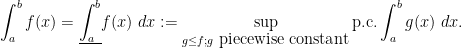
(It is also equal to the upper Darboux integral; but much as the theory of Lebesgue measure is easiest to define by relying solely on outer measure and not on inner measure, the theory of the unsigned Lebesgue integral is easiest to define by relying solely on lower integrals rather than upper ones; the upper integral is somewhat problematic when dealing with “improper” integrals of functions that are unbounded or are supported on sets of infinite measure.) Compare this formula also with (2). The integral is a piecewise constant integral, formed by breaking up the piecewise constant functions into finite linear combinations of indicator functions of intervals, and then measuring the length of each interval.

It turns out that virtually the same definition allows us to define a lower Lebesgue integral of any unsigned function , simply by replacing intervals with the more general class of Lebesgue measurable sets (and thus replacing piecewise constant functions with the more general class of simple functions). If the function is Lebesgue measurable (a concept that we will define presently), then we refer to the lower Lebesgue integral simply as the Lebesgue integral. As we shall see, it obeys all the basic properties one expects of an integral, such as monotonicity and additivity; in subsequent notes we will also see that it behaves quite well with respect to limits, as we shall see by establishing the two basic convergence theorems of the unsigned Lebesgue integral, namely Fatou’s lemma and the monotone convergence theorem.

Once we have the theory of the unsigned Lebesgue integral, we will then be able to define the absolutely convergent Lebesgue integral, similarly to how the absolutely convergent infinite sum can be defined using the unsigned infinite sum. This integral also obeys all the basic properties one expects, such as linearity and compatibility with the more classical Riemann integral; in subsequent notes we will see that it also obeys a fundamentally important convergence theorem, the dominated convergence theorem. This convergence theorem makes the Lebesgue integral (and its abstract generalisations to other measure spaces than ) particularly suitable for analysis, as well as allied fields that rely heavily on limits of functions, such as PDE, probability, and ergodic theory.

Remark 1 This is not the only route to setting up the unsigned and absolutely convergent Lebesgue integrals. Stein-Shakarchi, for instance, proceeds slightly differently, beginning with the unsigned integral but then making an auxiliary stop at integration of functions that are bounded and are supported on a set of finite measure, before going to the absolutely convergent Lebesgue integral. Another approach (which will not be discussed here) is to take the metric completion of the Riemann integral with respect to the metric.

The Lebesgue integral and Lebesgue measure can be viewed as completions of the Riemann integral and Jordan measure respectively. This means three things. Firstly, the Lebesgue theory extends the Riemann theory: every Jordan measurable set is Lebesgue measurable, and every Riemann integrable function is Lebesgue measurable, with the measures and integrals from the two theories being compatible. Conversely, the Lebesgue theory can be approximated by the Riemann theory; as we saw in the previous notes, every Lebesgue measurable set can be approximated (in various senses) by simpler sets, such as open sets or elementary sets, and in a similar fashion, Lebesgue measurable functions can be approximated by nicer functions, such as Riemann integrable or continuous functions. Finally, the Lebesgue theory is complete in various ways; we will formalise this properly only in the next quarter when we study spaces, but the convergence theorems mentioned above already hint at this completeness. A related fact, known as Egorov’s theorem, asserts that a pointwise converging sequence of functions can be approximated as a (locally) uniformly converging sequence of functions. The facts listed here manifestations of Littlewood’s three principles of real analysis, which capture much of the essence of the Lebesgue theory.

245A, Notes 1: Lebesgue measure

In the prologue for this course, we recalled the classical theory of Jordan measure on Euclidean spaces . This theory proceeded in the following stages:

1. First, one defined the notion of a box and its volume .
2. Using this, one defined the notion of an elementary set (a finite union of boxes), and defines the elementary measure of such sets.
3. From this, one defined the inner and outer Jordan measures of an arbitrary bounded set . If those measures match, we say that is Jordan measurable, and call the Jordan measure of .

As long as one is lucky enough to only have to deal with Jordan measurable sets, the theory of Jordan measure works well enough. However, as noted previously, not all sets are Jordan measurable, even if one restricts attention to bounded sets. In fact, we shall see later in these notes that there even exist bounded open sets, or compact sets, which are not Jordan measurable, so the Jordan theory does not cover many classes of sets of interest. Another class that it fails to cover is countable unions or intersections of sets that are already known to be measurable:

Exercise 1 Show that the countable union or countable intersection of Jordan measurable sets need not be Jordan measurable, even when bounded.

This creates problems with Riemann integrability (which, as we saw in the preceding notes, was closely related to Jordan measure) and pointwise limits:

Exercise 2 Give an example of a sequence of uniformly bounded, Riemann integrable functions for that converge pointwise to a bounded function that is not Riemann integrable. What happens if we replace pointwise convergence with uniform convergence?

These issues can be rectified by using a more powerful notion of measure than Jordan measure, namely Lebesgue measure. To define this measure, we first tinker with the notion of the Jordan outer measure

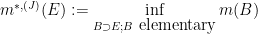
of a set (we adopt the convention that if is unbounded, thus now takes values in the extended non-negative reals , whose properties we will briefly review below). Observe from the finite additivity and subadditivity of elementary measure that we can also write the Jordan outer measure as

i.e. the Jordan outer measure is the infimal cost required to cover by a finite union of boxes. (The natural number is allowed to vary freely in the above infimum.) We now modify this by replacing the finite union of boxes by a countable union of boxes, leading to the Lebesgue outer measure of :

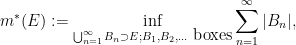
thus the Lebesgue outer measure is the infimal cost required to cover by a countable union of boxes. Note that the countable sum may be infinite, and so the Lebesgue outer measure could well equal .

(Caution: the Lebesgue outer measure is sometimes denoted ; this is for instance the case in Stein-Shakarchi.)

Clearly, we always have (since we can always pad out a finite union of boxes into an infinite union by adding an infinite number of empty boxes). But can be a lot smaller:

Example 1 Let be a countable set. We know that the Jordan outer measure of can be quite large; for instance, in one dimension, is infinite, and since has as its closure (see Exercise 18 of the prologue). On the other hand, all countable sets have Lebesgue outer measure zero. Indeed, one simply covers by the degenerate boxes of sidelength and volume zero.

Alternatively, if one does not like degenerate boxes, one can cover each by a cube of sidelength (say) for some arbitrary , leading to a total cost of , which converges to for some absolute constant . As can be arbitrarily small, we see that the Lebesgue outer measure must be zero. We will refer to this type of trick as the trick; it will be used many further times in this course.

From this example we see in particular that a set may be unbounded while still having Lebesgue outer measure zero, in contrast to Jordan outer measure.

As we shall see later in this course, Lebesgue outer measure (also known as Lebesgue exterior measure) is a special case of a more general concept known as an outer measure.

In analogy with the Jordan theory, we would also like to define a concept of “Lebesgue inner measure” to complement that of outer measure. Here, there is an asymmetry (which ultimately arises from the fact that elementary measure is subadditive rather than superadditive): one does not gain any increase in power in the Jordan inner measure by replacing finite unions of boxes with countable ones. But one can get a sort of Lebesgue inner measure by taking complements; see Exercise 18. This leads to one possible definition for Lebesgue measurability, namely the Carathéodory criterion for Lebesgue measurability, see Exercise 17. However, this is not the most intuitive formulation of this concept to work with, and we will instead use a different (but logically equivalent) definition of Lebesgue measurability. The starting point is the observation (see Exercise 5 of the prologue) that Jordan measurable sets can be efficiently contained in elementary sets, with an error that has small Jordan outer measure. In a similar vein, we will define Lebesgue measurable sets to be sets that can be efficiently contained in open sets, with an error that has small Lebesgue outer measure:

Definition 1 (Lebesgue measurability) A set is said to be Lebesgue measurable if, for every , there exists an open set containing such that . If is Lebesgue measurable, we refer to as the Lebesgue measure of (note that this quantity may be equal to ). We also write as when we wish to emphasise the dimension .

(The intuition that measurable sets are almost open is also known as Littlewood’s first principle, this principle is a triviality with our current choice of definitions, though less so if one uses other, equivalent, definitions of Lebesgue measurability.)

As we shall see later, Lebesgue measure extends Jordan measure, in the sense that every Jordan measurable set is Lebesgue measurable, and the Lebesgue measure and Jordan measure of a Jordan measurable set are always equal. We will also see a few other equivalent descriptions of the concept of Lebesgue measurability.

In the notes below we will establish the basic properties of Lebesgue measure. Broadly speaking, this concept obeys all the intuitive properties one would ask of measure, so long as one restricts attention to countable operations rather than uncountable ones, and as long as one restricts attention to Lebesgue measurable sets. The latter is not a serious restriction in practice, as almost every set one actually encounters in analysis will be measurable (the main exceptions being some pathological sets that are constructed using the axiom of choice). In the next set of notes we will use Lebesgue measure to set up the Lebesgue integral, which extends the Riemann integral in the same way that Lebesgue measure extends Jordan measure; and the many pleasant properties of Lebesgue measure will be reflected in analogous pleasant properties of the Lebesgue integral (most notably the convergence theorems).

We will treat all dimensions equally here, but for the purposes of drawing pictures, we recommend to the reader that one sets equal to . However, for this topic at least, no additional mathematical difficulties will be encountered in the higher-dimensional case (though of course there are significant visual difficulties once exceeds ).

The material here is based on Sections 1.1-1.3 of the Stein-Shakarchi text, though it is arranged somewhat differently.

245A, prologue: The problem of measure

One of the most fundamental concepts in Euclidean geometry is that of the measure of a solid body in one or more dimensions. In one, two, and three dimensions, we refer to this measure as the length, area, or volume of respectively. In the classical approach to geometry, the measure of a body was often computed by partitioning that body into finitely many components, moving around each component by a rigid motion (e.g. a translation or rotation), and then reassembling those components to form a simpler body which presumably has the same area. One could also obtain lower and upper bounds on the measure of a body by computing the measure of some inscribed or circumscribed body; this ancient idea goes all the way back to the work of Archimedes at least. Such arguments can be justified by an appeal to geometric intuition, or simply by postulating the existence of a measure that can be assigned to all solid bodies , and which obeys a collection of geometrically reasonable axioms. One can also justify the concept of measure on “physical” or “reductionistic” grounds, viewing the measure of a macroscopic body as the sum of the measures of its microscopic components.

With the advent of analytic geometry, however, Euclidean geometry became reinterpreted as the study of Cartesian products of the real line . Using this analytic foundation rather than the classical geometrical one, it was no longer intuitively obvious how to define the measure of a general subset of ; we will refer to this (somewhat vaguely defined) problem of writing down the “correct” definition of measure as the problem of measure. (One can also pose the problem of measure on other domains than Euclidean space, such as a Riemannian manifold, but we will focus on the Euclidean case here for simplicity.)

To see why this problem exists at all, let us try to formalise some of the intuition for measure discussed earlier. The physical intuition of defining the measure of a body to be the sum of the measure of its component “atoms” runs into an immediate problem: a typical solid body would consist of an infinite (and uncountable) number of points, each of which has a measure of zero; and the product is indeterminate. To make matters worse, two bodies that have exactly the same number of points, need not have the same measure. For instance, in one dimension, the intervals and are in one-to-one correspondence (using the bijection from to ), but of course is twice as long as . So one can disassemble into an uncountable number of points and reassemble them to form a set of twice the length.

Of course, one can point to the infinite (and uncountable) number of components in this disassembly as being the cause of this breakdown of intuition, and restrict attention to just finite partitions. But one still runs into trouble here for a number of reasons, the most striking of which is the Banach-Tarski paradox, which shows that the unit ball in three dimensions can be disassembled into a finite number of pieces (in fact, just five pieces suffice), which can then be reassembled (after translating and rotating each of the pieces) to form two disjoint copies of the ball . (The paradox only works in three dimensions and higher, for reasons having to do with the property of amenability; see this blog post for further discussion of this interesting topic, which is unfortunately too much of a digression from the current subject.)

Here, the problem is that the pieces used in this decomposition are highly pathological in nature; among other things, their construction requires use of the axiom of choice. (This is in fact necessary; there are models of set theory without the axiom of choice in which the Banach-Tarski paradox does not occur, thanks to a famous theorem of Solovay.) Such pathological sets almost never come up in practical applications of mathematics. Because of this, the standard solution to the problem of measure has been to abandon the goal of measuring every subset of , and instead to settle for only measuring a certain subclass of “non-pathological” subsets of , which are then referred to as the measurable sets. The problem of measure then divides into several subproblems:

1. What does it mean for a subset of to be measurable?
2. If a set is measurable, how does one define its measure?
3. What nice properties or axioms does measure (or the concept of measurability) obey?
4. Are “ordinary” sets such as cubes, balls, polyhedra, etc. measurable?
5. Does the measure of an “ordinary” set equal the “naive geometric measure” of such sets? (e.g. is the measure of an rectangle equal to ?)

These questions are somewhat open-ended in formulation, and there is no unique answer to them; in particular, one can expand the class of measurable sets at the expense of losing one or more nice properties of measure in the process (e.g. finite or countable additivity, translation invariance, or rotation invariance). However, there are two basic answers which, between them, suffice for most applications. The first is the concept of Jordan measure of a Jordan measurable set, which is a concept closely related to that of the Riemann integral (or Darboux integral). This concept is elementary enough to be systematically studied in an undergraduate analysis course, and suffices for measuring most of the “ordinary” sets (e.g. the area under the graph of a continuous function) in many branches of mathematics. However, when one turns to the type of sets that arise in analysis, and in particular those sets that arise as limits (in various senses) of other sets, it turns out that the Jordan concept of measurability is not quite adequate, and must be extended to the more general notion of Lebesgue measurability, with the corresponding notion of Lebesgue measure that extends Jordan measure. With the Lebesgue theory (which can be viewed as a completion of the Jordan-Darboux-Riemann theory), one keeps almost all of the desirable properties of Jordan measure, but with the crucial additional property that many features of the Lebesgue theory are preserved under limits (as exemplified in the fundamental convergence theorems of the Lebesgue theory, such as the monotone convergence theorem and the dominated convergence theorem, which do not hold in the Jordan-Darboux-Riemann setting). As such, they are particularly well suited for applications in analysis, where limits of functions or sets arise all the time. (There are other ways to extend Jordan measure and the Riemann integral, but the Lebesgue approach handles limits better than the other alternatives, and so has become the standard approach in analysis.)

In the rest of the course, we will formally define Lebesgue measure and the Lebesgue integral, as well as the more general concept of an abstract measure space and the associated integration operation. In the rest of this post, we will discuss the more elementary concepts of Jordan measure and the Riemann integral. This material will eventually be superceded by the more powerful theory to be treated in the main body of the course; but it will serve as motivation for that later material, as well as providing some continuity with the treatment of measure and integration in undergraduate analysis courses.