Princeton Companion to Mathematics

The Princeton Companion to Mathematics Sample Entry: Fermat’s Last Theorem Podcast interview with editor Timothy Gowers

I was very pleased today to obtain a courtesy copy of the Princeton Companion to Mathematics, which is now in print.  I have discussed several of the individual articles (including my own) in this book elsewhere in this blog, and Tim Gowers, the main editor of the Companion, has of course also discussed it on his blog.  Browsing through it, though, I do get the sense that the whole is greater than the sum of its parts. One particularly striking example of this is the final section on advice to younger mathematicians, with contributions by Sir Michael Atiyah, Béla Bollobás, Alain Connes, Dusa McDuff, and Peter Sarnak; the individual contributions are already very insightful (and almost linearly independent of each other!), but collectively they give a remarkably comprehensive and accurate portrait of how mathematical progress is made these days.

The other immediate impression I got from the book was the sheer weight (physical and otherwise – the book comprises 1034 pages) of mathematics that is out there, much of which I still only have a very partial grasp of at best (see also Einstein’s famous quote on the subject).  But the book also demonstrates that mathematics, while large, is at least connected (and reasonably bounded in diameter, modulo a small exceptional set).  I myself certainly plan to use this book as a first reference the next time I need to look up some mathematical theory or concept that I haven’t had occasion to really use much before.

Given that I have been heavily involved in certain parts of this project, I will not review the book fully here – I am sure that will be done more objectively elsewhere – but comments on the book by other readers are more than welcome here.

[Update, Sep 29: link to advice chapter added.]

What is a gauge?

“Gauge theory” is a term which has connotations of being a fearsomely complicated part of mathematics – for instance, playing an important role in quantum field theory, general relativity, geometric PDE, and so forth.  But the underlying concept is really quite simple: a gauge is nothing more than a “coordinate system” that varies depending on one’s “location” with respect to some “base space” or “parameter space”, a gauge transform is a change of coordinates applied to each such location, and a gauge theory is a model for some physical or mathematical system to which gauge transforms can be applied (and is typically gauge invariant, in that all physically meaningful quantities are left unchanged (or transform naturally) under gauge transformations).  By fixing a gauge (thus breaking or spending the gauge symmetry), the model becomes something easier to analyse mathematically, such as a system of partial differential equations (in classical gauge theories) or a perturbative quantum field theory (in quantum gauge theories), though the tractability of the resulting problem can be heavily dependent on the choice of gauge that one fixed.  Deciding exactly how to fix a gauge (or whether one should spend the gauge symmetry at all) is a key question in the analysis of gauge theories, and one that often requires the input of geometric ideas and intuition into that analysis.

I was asked recently to explain what a gauge theory was, and so I will try to do so in this post.  For simplicity, I will focus exclusively on classical gauge theories; quantum gauge theories are the quantization of classical gauge theories and have their own set of conceptual difficulties (coming from quantum field theory) that I will not discuss here. While gauge theories originated from physics, I will not discuss the physical significance of these theories much here, instead focusing just on their mathematical aspects.  My discussion will be informal, as I want to try to convey the geometric intuition rather than the rigorous formalism (which can, of course, be found in any graduate text on differential geometry).

The divisor bound

Given a positive integer , let denote the number of divisors of n (including 1 and n), thus for instance d(6)=4, and more generally, if n has a prime factorisation

(1)

then (by the fundamental theorem of arithmetic)

. (2)

Clearly, .  The divisor bound asserts that, as gets large, one can improve this trivial bound to

(3)

for any , where depends only on ; equivalently, in asymptotic notation one has .  In fact one has a more precise bound

. (4)

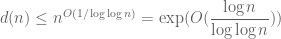
The divisor bound is useful in many applications in number theory, harmonic analysis, and even PDE (on periodic domains); it asserts that for any large number n, only a “logarithmically small” set of numbers less than n will actually divide n exactly, even in the worst-case scenario when n is smooth.  (The average value of d(n) is much smaller, being about on the average, as can be seen easily from the double counting identity

,

or from the heuristic that a randomly chosen number m less than n has a probability about 1/m of dividing n, and .  However, (4) is the correct “worst case” bound, as I discuss below.)

The divisor bound is elementary to prove (and not particularly difficult), and I was asked about it recently, so I thought I would provide the proof here, as it serves as a case study in how to establish worst-case estimates in elementary multiplicative number theory.

[Update, Sep 24: some applications added.]

On hiatus

Due to various other things that have come up, I will be cutting back on my blogging for a while.  I hope to resume here in a couple weeks, though.

Oded Schramm

I am very saddened (and stunned) to learn that Oded Schramm, who made fundamental contributions to conformal geometry, probability theory, and mathematical physics, died in a hiking accident this Monday, aged 46.  (I knew him as a fellow editor of the Journal of the American Mathematical Society, as well as for his mathematical research, of course.)  It is a loss of both a great mathematician and a great person.

One of Schramm’s most fundamental contributions to mathematics is the introduction of the stochastic Loewner equation (now sometimes called the Schramm-Loewner equation in his honour), together with his subsequent development of the theory of this equation with Greg Lawler and Wendelin Werner.  (This work has been recognised by a number of awards, including the Fields Medal in 2006 to Wendelin.)  This equation (which I state after the jump) describes, for each choice of a parameter , a random (fractal) curve in the plane; this random curve can be viewed as a nonlinear variant of Brownian motion, although the SLE curves tend to cross themselves much less frequently than Brownian paths do.  By the nature of their construction, the curves are conformally invariant: any conformal transformation of an curve (respecting the boundary) gives another curve which has the same distribution as the original curve.  (Brownian motion is also conformally invariant; given the close connections between Brownian motion and harmonic functions, it is not surprising that this fact is closely related to the fact that the property of a function being harmonic in the plane is preserved under conformal transformations.) Conversely, one can show that any conformally invariant random curve distribution which obeys some additional regularity and locality axioms must be of the form for some .

The amazing fact is that many other natural processes for generating random curves in the plane – e.g. loop-erased random walk, the boundary of Brownian motion (also known as the “Brownian frontier”), or the limit of percolation on the triangular lattice – are known or conjectured to be distributed according to for some specific (in the above three examples, is 2, 8/3, and 6 respectively).  In particular, this implies that the highly non-trivial fact that such distributions are conformally invariant, a phenomenon that had been conjectured by physicists but which only obtained rigorous mathematical proof following the work of Schramm and his coauthors.

[Update, Sep 6: A memorial blog to Oded has been set up by his Microsoft Research group here.  See also these posts by Gil Kalai, Yuval Peres, and Luca Trevisan.]