You are currently browsing the tag archive for the ‘Ricci flow’ tag.

Peter Petersen and I have just uploaded to the arXiv our paper, “Classification of Almost Quarter-Pinched Manifolds“, submitted to Proc. Amer. Math. Soc..  This is perhaps the shortest paper (3 pages) I have ever been involved in, because we were fortunate enough that we could simply cite (as a black box) a reference for every single fact that we needed here.

The paper is related to the famous sphere theorem from Riemannian geometry.  This theorem asserts that any n-dimensional complete simply connected Riemannian manifold which was strictly quarter-pinched (i.e. the sectional curvatures all in the interval (K/4,K] for some K > 0) must necessarily be homeomorphic to the n-sphere S^n.    (In dimensions 3 or less, this already follows from simple connectedness thanks to the Poincaré conjecture (and Myers theorem), so the theorem is really only interesting in higher dimensions.  One can easily drop the simple connectedness hypothesis by passing to a universal cover, but then one has to admit sphere quotients S^n/\Gamma as well as spheres.)

Due to the existence of exotic spheres in higher dimensions, being homeomorphic to a sphere does not necessarily imply being diffeomorphic to a sphere.  (For instance, an example of an exotic sphere with positive sectional curvature (but not quarter-pinched) was recently constructed by Petersen and Wilhelm.)  Nevertheless, Brendle and Schoen recently proved the diffeomorphic version of the sphere theorem: every strictly quarter-pinched complete simply connected Riemannian manifold is diffeomorphic to a sphere.  The proof is based on Ricci flow, and involves three main steps:

  1. A verification that if M is quarter-pinched, then the manifold M \times {\Bbb R}^2 has non-negative isotropic curvature.  (The same statement is true without adding the two additional flat dimensions, but these additional dimensions are very convenient for simplifying the analysis by allowing certain two-planes to wander freely in the product tangent space.)
  2. A verification that the property of having non-negative isotropic curvature is preserved by Ricci flow.  (By contrast, the quarter-pinched property is not preserved by Ricci flow.)
  3. The pinching theory of Böhm and Wilking, which is a refinement of the work of Hamilton (who handled the three and four-dimensional cases).

Brendle and Schoen in fact proved a slightly stronger statement in which the curvature bound K is allowed to vary with position x, but we will not discuss this strengthening here.

The quarter-pinching is sharp; the Fubini-Study metric on complex projective spaces {\Bbb CP}^n is non-strictly quarter-pinched (the sectional curvatures lie in {}[K/4,K] but is not homeomorphic to a sphere).  Nevertheless, by refining the above methods, an endpoint result was established by Brendle and Schoen (see also a later refinement by Seshadri): any complete simply-connected manifold which is non-strictly quarter-pinched is diffeomorphic to either a sphere or a compact rank one symmetric space (or CROSS, for short) such as complex projective space.  (In the latter case one also has some further control on the metric, which we will not detail here.)  The homeomorphic version of this statement was established earlier by Berger and by Klingenberg.

Our result pushes this further by an epsilon.  More precisely, we show for each dimension n that there exists \varepsilon > 0 such that any \frac{1}{4}-\varepsilon_n-pinched complete simply connected manifold (i.e. the curvatures lie in {}[K (\frac{1}{4}-\varepsilon_n), K]) is diffeomorphic to either a sphere or a CROSS.  (The homeomorphic version of this statement was established earlier in even dimensions by Berger.)  We do not know if \varepsilon_n can be made independent of n.

Read the rest of this entry »

We continue our study of \kappa-solutions. In the previous lecture we primarily exploited the non-negative curvature of such solutions; in this lecture and the next, we primarily exploit the ancient nature of these solutions, together with the finer analysis of the two scale-invariant monotone quantities we possess (Perelman entropy and Perelman reduced volume) to obtain a important scaling limit of \kappa-solutions, the asymptotic gradient shrinking soliton of such a solution.

The main idea here is to exploit what I have called the infinite convergence principle in a previous post: that every bounded monotone sequence converges. In the context of \kappa-solutions, we can apply this principle to either of our monotone quantities: the Perelman entropy

\displaystyle \mu(g(t),\tau) := \inf \{ {\mathcal W}(M,g(t),f,\tau): \int_M (4\pi\tau)^{-d/2} e^{-f}\ d\mu = 1 \} (1)

where \tau := -t is the backwards time variable and

\displaystyle {\mathcal W}(M,g(t),f,\tau) := \int_M (\tau(|\nabla f|^2 + R) + f - d) (4\pi\tau)^{-d/2} e^{-f}\ d\mu, (2)

or the Perelman reduced volume
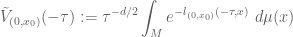
\displaystyle \tilde V_{(0,x_0)}(-\tau) := \tau^{-d/2} \int_M e^{-l_{(0,x_0)}(-\tau,x)}\ d\mu(x) (3)

where x_0 \in M is a fixed base point. As pointed out in Lecture 11, these quantities are related, and both are non-increasing in \tau.

The reduced volume starts off at (4\pi)^{d/2} when \tau=0, and so by the infinite convergence principle it approaches some asymptotic limit 0 \leq \tilde V_{(0,x_0)}(-\infty) \leq (4\pi)^{d/2} as \tau \to -\infty. (We will later see that this limit is strictly between 0 and (4\pi)^{d/2}.) On the other hand, the reduced volume is invariant under the scaling

g^{(\lambda)}(t) := \frac{1}{\lambda^2} g( \lambda^2 t ), (4)

in the sense that

\tilde V_{(0,x_0)}^{(\lambda)}(-\tau) = \tilde V_{(0,x_0)}(-\lambda^2 \tau). (5)

Thus, as we send \lambda \to \infty, the reduced volumes of the rescaled flows t \mapsto (M, g^{(\lambda)}(t)) (which are also \kappa-solutions) converge pointwise to a constant \tilde V_{(0,x_0)}(-\infty).

Suppose that we could somehow “take a limit” of the flows t \mapsto (M, g^{(\lambda)}(t)) (or perhaps a subsequence of such flows) and obtain some limiting flow t \mapsto (M^{(\infty)}, g^{(\infty)}(t)). Formally, such a flow would then have a constant reduced volume of \tilde V_{(0,x_0)}(-\infty). On the other hand, the reduced volume is monotone. If we could have a criterion as to when the reduced volume became stationary, we could thus classify all possible limiting flows t \mapsto (M^{(\infty)}, g^{(\infty)}(t)), and thus obtain information about the asymptotic behaviour of \kappa-solutions (at least along a subsequence of scales going to infinity).

We will carry out this program more formally in the next lecture, in which we define the concept of an asymptotic gradient-shrinking soliton of a \kappa-solution.
In this lecture, we content ourselves with a key step in this program, namely to characterise when the Perelman entropy or Perelman reduced volume becomes stationary; this requires us to revisit the theory we have built up in the last few lectures. It turns out that, roughly speaking, this only happens when the solution is a gradient shrinking soliton, thus at any given time -\tau one has an equation of the form \hbox{Ric} + \hbox{Hess}(f) = \lambda g for some f: M \to {\Bbb R} and \lambda > 0. Our computations here will be somewhat formal in nature; we will make them more rigorous in the next lecture.

The material here is largely based on Morgan-Tian’s book and the first paper of Perelman. Closely related treatments also appear in the notes of Kleiner-Lott and the paper of Cao-Zhu.

Read the rest of this entry »

We now turn to the theory of parabolic Harnack inequalities, which control the variation over space and time of solutions to the scalar heat equation

u_t = \Delta u (1)

which are bounded and non-negative, and (more pertinently to our applications) of the curvature of Ricci flows

g_t = -2\hbox{Ric} (2)

whose Riemann curvature \hbox{Riem} or Ricci curvature \hbox{Ric} is bounded and non-negative. For instance, the classical parabolic Harnack inequality of Moser asserts, among other things, that one has a bound of the form

u(t_1,x_1) \leq C(t_1,x_1,t_0,x_0,T_-,T_+,M) u(t_0,x_0) (3)

whenever u: [T_-,T_+] \times M \to {\Bbb R}^+ is a bounded non-negative solution to (1) on a complete static Riemannian manifold M of bounded curvature, (t_1,x_1), (t_0,x_0) \in [T_-,T_+] \times M are spacetime points with t_1 < t_0, and C(t_1,x_1,t_0,x_0,T_-,T_+,M) is a constant which is uniformly bounded for fixed t_1,t_0,T_-,T_+,M when x_1,x_0 range over a compact set. (The even more classical elliptic Harnack inequality gives (1) in the steady state case, i.e. for bounded non-negative harmonic functions.) In terms of heat kernels, one can view (1) as an assertion that the heat kernel associated to (t_0,x_0) dominates (up to multiplicative constants) the heat kernel at (t_1,x_1).

The classical proofs of the parabolic Harnack inequality do not give particularly sharp bounds on the constant C(t_1,x_1,t_0,x_0,T_-,T_+,M). Such sharp bounds were obtained by Li and Yau, especially in the case of the scalar heat equation (1) in the case of static manifolds of non-negative Ricci curvature, using Bochner-type identities and the scalar maximum principle. In fact, a stronger differential version of (3) was obtained which implied (3) by an integration along spacetime curves (closely analogous to the {\mathcal L}-geodesics considered in earlier lectures). These bounds were particularly strong in the case of ancient solutions (in which one can send T_- \to -\infty). Subsequently, Hamilton applied his tensor-valued maximum principle together with some remarkably delicate tensor algebra manipulations to obtain Harnack inequalities of Li-Yau type for solutions to the Ricci flow (2) with bounded non-negative Riemannian curvature. In particular, this inequality applies to the \kappa-solutions introduced in the previous lecture.

In this current lecture, we shall discuss all of these inequalities (although we will not give the full details for the proof of Hamilton’s Harnack inequality, as the computations are quite involved), and derive several important consequences of that inequality for \kappa-solutions. The material here is based on several sources, including Evans’ PDE book, Müller’s book, Morgan-Tian’s book, the paper of Cao-Zhu, and of course the primary source papers mentioned in this article.

Read the rest of this entry »

Having established the monotonicity of the Perelman reduced volume in the previous lecture (after first heuristically justifying this monotonicity in Lecture 9), we now show how this can be used to establish \kappa-noncollapsing of Ricci flows, thus giving a second proof of Theorem 2 from Lecture 7. Of course, we already proved (a stronger version) of this theorem already in Lecture 8, using the Perelman entropy, but this second proof is also important, because the reduced volume is a more localised quantity (due to the weight e^{-l_{(0,x_0)}} in its definition and so one can in fact establish local versions of the non-collapsing theorem which turn out to be important when we study ancient \kappa-noncollapsing solutions later in Perelman’s proof, because such solutions need not be compact and so cannot be controlled by global quantities (such as the Perelman entropy).

The route to \kappa-noncollapsing via reduced volume proceeds by the following scheme:

Non-collapsing at time t=0 (1)

\Downarrow

Large reduced volume at time t=0 (2)

\Downarrow

Large reduced volume at later times t (3)

\Downarrow

Non-collapsing at later times t (4)

The implication (2) \implies (3) is the monotonicity of Perelman reduced volume. In this lecture we discuss the other two implications (1) \implies (2), and (3) \implies (4)).

Our arguments here are based on Perelman’s first paper, Kleiner-Lott’s notes, and Morgan-Tian’s book, though the material in the Morgan-Tian book differs in some key respects from the other two texts. A closely related presentation of these topics also appears in the paper of Cao-Zhu.

Read the rest of this entry »

In this lecture we discuss Perelman’s original approach to finite time extinction of the third homotopy group (Theorem 1 from the previous lecture), which, as previously discussed, can be combined with the finite time extinction of the second homotopy group to imply finite time extinction of the entire Ricci flow with surgery for any compact simply connected Riemannian 3-manifold, i.e. Theorem 4 from Lecture 2.

Read the rest of this entry »

Returning (perhaps anticlimactically) to the subject of the Poincaré conjecture, recall from Lecture 2 that one of the key pillars of the proof of that conjecture is the finite time extinction result (see Theorem 4 from that lecture), which asserted that if a compact Riemannian 3-manifold (M,g) was initially simply connected, then after a finite amount of time evolving via Ricci flow with surgery, the manifold will be empty.

In this lecture and the next few, we will describe some of the key ideas used to prove this theorem. We will not be able to completely establish this theorem at present, because we do not have a full definition of “surgery”, but we will be able to establish some partial results, and indicate (in informal terms) how to cope with the additional technicalities caused by the surgery procedure. Hopefully, if time permits later in the class, once we have studied the surgery process, I will be able to revisit this material and flesh out these technicalities a bit more.

The proof of finite time extinction proceeds in several stages. The first stage, which was already accomplished in the previous lecture (in the absence of surgery, at least), is to establish lower bounds on the least scalar curvature R_{\min}. The next stage, which we discuss in this lecture, is to show that the second homotopy group \pi_2(M) of the manifold must become extinct in finite time, thus all immersed copies of the 2-sphere S^2 in M(t) for sufficiently large t must be contractible to a point. The third stage is to show that the third homotopy group \pi_3(M) also becomes extinct so that all immersed copies of the 3-sphere S^3 in M are similarly contractible. The final stage, which uses homology theory, is to show that a non-empty 3-manifold cannot have \pi_1(M), \pi_2(M), \pi_3(M) simultaneously trivial, thus yielding the desired claim (note that a simply connected manifold has trivial \pi_1(M) by definition; also, from Exercise 2 of Lecture 2 we see that all components of M remain simply connected even after surgery).

More precisely, in this lecture we will discuss (most of) the proof of

Theorem 1. (Finite time extinction of \pi_2(M)) Let t \mapsto (M(t),g(t)) be a Ricci flow with surgery on compact 3-manifolds with t \in [0,+\infty), with M(0) containing no embedded copy of \Bbb{RP}^2 with trivial normal bundle. Then for all sufficiently large t, \pi_2(M(t)) is trivial (or more precisely, every connected component of M(t) has trivial \pi_2).

The technical assumption about having no copy of \Bbb{RP}^2 with trivial normal bundle is needed solely in order to apply the known existence theory for Ricci flow with surgery (see Theorem 2 from Lecture 2).

The intuition for this result is as follows. From the Gauss-Bonnet theorem (and the fact that the Euler characteristic \chi(S^2)=V-E+F=2 of the sphere is positive), we know that 2-spheres tend to have positive (Gaussian) curvature on the average, which should make them shrink under Ricci flow. (Here I am conflating Gaussian curvature with Ricci curvature; however, by restricting to a special class of 2-spheres, namely minimal surfaces, one can connect the two notions of curvature to each other (and to scalar curvature) quite nicely.) On the other hand, the presence of negative scalar curvature can counteract this by expanding these spheres. But the lower bounds on scalar curvature tell us that the negativity of scalar curvature becomes weakened over time, and it turns out that the shrinkage caused by the Gauss-Bonnet theorem eventually dominates and sends the area of all minimal immersed 2-spheres into zero, at which point one can conclude the triviality of \pi_2(M) by the Sacks-Uhlenbeck theory of minimal 2-spheres.

The arguments here are drawn from the book of Morgan-Tian and from the paper of Colding-Minicozzi. The idea of using minimal surfaces to force disappearance of various topological structures under Ricci flow originates with Hamilton (who used 2-torii instead of 2-spheres, but the idea is broadly the same).

Read the rest of this entry »

We now begin the study of (smooth) solutions t \mapsto (M(t),g(t)) to the Ricci flow equation

\frac{d}{dt} g_{\alpha \beta} = - 2 \hbox{Ric}_{\alpha \beta}, (1)

particularly for compact manifolds in three dimensions. Our first basic tool will be the maximum principle for parabolic equations, which we will use to bound (sub-)solutions to nonlinear parabolic PDE by (super-)solutions, and vice versa. Because the various curvatures \hbox{Riem}_{\alpha \beta \gamma}^\delta, \hbox{Ric}_{\alpha \beta}, R of a manifold undergoing Ricci flow do indeed obey nonlinear parabolic PDE (see equations (31) from Lecture 1), we will be able to obtain some important lower bounds on curvature, and in particular establishes that the curvature is either bounded, or else that the positive components of the curvature dominate the negative components. This latter phenomenon, known as the Hamilton-Ivey pinching phenomenon, is particularly important when studying singularities of Ricci flow, as it means that the geometry of such singularities is almost completely dominated by regions of non-negative (and often quite high) curvature.

Read the rest of this entry »

In the first lecture, we introduce flows t \mapsto (M(t), g(t)) on Riemannian manifolds (M,g), which are recipes for describing smooth deformations of such manifolds over time, and derive the basic first variation formulae for how various structures on such manifolds (e.g. curvature, length, volume) change by such flows. (One can view these formulae as describing the relationship between two “infinitesimally close” Riemannian manifolds.) We then specialise to the case of Ricci flow (together with some close relatives of this flow, such as renormalised Ricci flow, or Ricci flow composed with a diffeomorphism flow). We also discuss the “de Turck trick” that modifies the Ricci flow into a nonlinear parabolic equation, for the purposes of establishing local existence and uniqueness of that flow.

Read the rest of this entry »

I’m closing my series of articles for the Princeton Companion to Mathematics with my article on “Ricci flow“. Of course, this flow on Riemannian manifolds is now very well known to mathematicians, due to its fundamental role in Perelman’s celebrated proof of the Poincaré conjecture. In this short article, I do not focus on that proof, but instead on the more basic questions as to what a Riemannian manifold is, what the Ricci curvature tensor is on such a manifold, and how Ricci flow qualitatively changes the geometry (and with surgery, the topology) of such manifolds over time.

I’ve saved this article for last, in part because it ties in well with my upcoming course on Perelman’s proof which will start in a few weeks (details to follow soon).

The last external article for the PCM that I would like to point out here is Brian Osserman‘s article on the Weil conjectures, which include the “Riemann hypothesis over finite fields” that was famously solved by Deligne. These (now solved) conjectures, which among other things gives some quite precise control on the number of points in an algebraic variety over a finite field, were (and continue to be) a major motivating force behind much of modern arithmetic and algebraic geometry.

[Update, Mar 13: Actual link to Weil conjecture article added.]

On Friday, Yau concluded his lecture series by discussing the PDE approach to constructing geometric structures, particularly Einstein metrics, and their applications to many questions in low-dimensional topology (yes, this includes the Poincaré conjecture). Yau also discussed the situation in high-dimensional topology, which appears to be completely different (and much less well understood).

Yau’s slides for this talk are available here.

Read the rest of this entry »

Archives