
You are currently browsing the tag archive for the ‘prime number theorem’ tag.
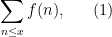
Previous set of notes: Notes 3. Next set of notes: 246C Notes 1.
One of the great classical triumphs of complex analysis was in providing the first complete proof (by Hadamard and de la Vallée Poussin in 1896) of arguably the most important theorem in analytic number theory, the prime number theorem:
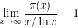
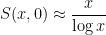
Theorem 1 (Prime number theorem) Letdenote the number of primes less than a given real number
. Then
(or in asymptotic notation,
as
).
(Actually, it turns out to be slightly more natural to replace the approximation 

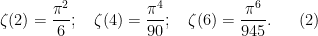
The complex-analytic proof of this theorem hinges on the study of a key meromorphic function related to the prime numbers, the Riemann zeta function 
Definition 2 (Riemann zeta function, preliminary definition) Letbe such that
. Then we define

Note that the series is locally uniformly convergent in the half-plane
The Riemann zeta function has several remarkable properties, some of which we summarise here:
Theorem 3 (Basic properties of the Riemann zeta function)
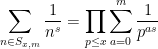
- (i) (Euler product formula) For any
where the product is absolutely convergent (and locally uniform in
) and is over the prime numbers
.
- (ii) (Trivial zero-free region)
has no zeroes in the region
.
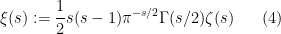
- (iii) (Meromorphic continuation)
and no other poles. Furthermore, the Riemann xi function
is an entire function of order
(after removing all singularities). The function
is an entire function of order one after removing the singularity at
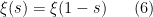
- (iv) (Functional equation) After applying the meromorphic continuation from (iii), we have
for all
for all


Proof: We just prove (i) and (ii) for now, leaving (iii) and (iv) for later sections.
The claim (i) is an encoding of the fundamental theorem of arithmetic, which asserts that every natural number 


 ,
,  , and
, and  consists of all the natural numbers of the form
  for some
  . Sending
  and to infinity, we conclude from monotone convergence and the geometric series formula that
 is real, and then from dominated convergence we see that the same formula holds for complex with as well. Local uniform convergence then follows from the product form of the Weierstrass
  -test (Exercise 19 of Notes 1).
The claim (ii) is immediate from (i) since the Euler product 

We remark that by sending
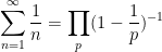
 . This can be viewed as a weak version of the prime number theorem, and already illustrates the potential applicability of the Riemann zeta function to control the distribution of the prime numbers.
The meromorphic continuation (iii) of the zeta function is initially surprising, but can be interpreted either as a manifestation of the extremely regular spacing of the natural numbers 
Henceforth we work with the meromorphic continuation of 


From Theorem 3 and the non-vanishing nature of 


 by (1), hence for all (except the pole at ) by meromorphic continuation. Thus if is a non-trivial zero then so is
  . We conclude that the set of non-trivial zeroes is symmetric by reflection by both the real axis and the critical line
 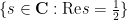 . We have the following infamous conjecture:
Conjecture 4 (Riemann hypothesis) All the non-trivial zeroes of
This conjecture would have many implications in analytic number theory, particularly with regard to the distribution of the primes. Of course, it is far from proven at present, but the partial results we have towards this conjecture are still sufficient to establish results such as the prime number theorem.
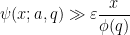
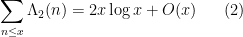
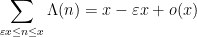
Return now to the original region where


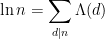
 , where the von Mangoldt function
  is defined to equal
  whenever
  is a power
  of a prime
  for some
  , and
, and  otherwise. The contribution of the higher prime powers
  is negligible in practice, and as a first approximation one can think of the von Mangoldt function as the indicator function of the primes, weighted by the logarithm function.
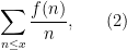
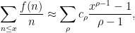
The series 

Exercise 5 (Standard Dirichlet series) Let
- (i) Show that
.
- (ii) Show that
, where
is the divisor function of
- (iii) Show that
, where
is the Möbius function, defined to equal
when
distinct primes for some
, and
otherwise.
- (iv) Show that
, where
is the Liouville function, defined to equal
- (v) Show that
, where
is the holomorphic branch of the logarithm that is real for
vanishes for
.
- (vi) Use the fundamental theorem of arithmetic to show that the von Mangoldt function is the unique function
such that
for every positive integer
Given the appearance of the von Mangoldt function 
Theorem 6 (Prime number theorem, von Mangoldt form) One has(or in asymptotic notation,
as
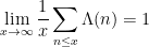
Let us see how Theorem 6 implies Theorem 1. Firstly, for any 
 is non-zero for only
  values of
  , and is of size
  , thus
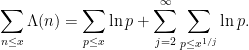
 , we conclude from Theorem 6 that
  . Next, observe from the fundamental theorem of calculus that
 and summing over all primes
  , we conclude that
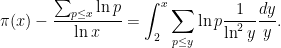
 , thus
 and
and  we see that the right-hand side is
  , and Theorem 1 follows.
Exercise 7 Show that Theorem 1 conversely implies Theorem 6.
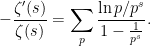
The alternate form (8) of the Euler product identity connects the primes (represented here via proxy by the von Mangoldt function) with the logarithmic derivative of the zeta function, and can be used as a starting point for describing further relationships between
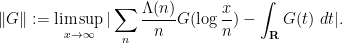
Theorem 8 (Riemann-von Mangoldt explicit formula) For any non-integer, we have
where
. Furthermore, the convergence of the limit is locally uniform in

Actually, it turns out that this formula is in some sense too precise; in applications it is often more convenient to work with smoothed variants of this formula in which the sum on the left-hand side is smoothed out, but the contribution of zeroes with large imaginary part is damped; see Exercise 22. Nevertheless, this formula clearly illustrates how the non-trivial zeroes

 )
) 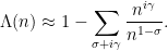
 induces an oscillation in the von Mangoldt function, with
  controlling the frequency of the oscillation and
  the rate to which the oscillation dies out as
  . This relationship is sometimes known informally as “the music of the primes”.
Comparing Theorem 8 with Theorem 6, it is natural to suspect that the key step in the proof of the latter is to establish the following slight but important extension of Theorem 3(ii), which can be viewed as a very small step towards the Riemann hypothesis:
Theorem 9 (Slight enlargement of zero-free region) There are no zeroes of.
It is not quite immediate to see how Theorem 6 follows from Theorem 8 and Theorem 9, but we will demonstrate it below the fold.
Although Theorem 9 only seems like a slight improvement of Theorem 3(ii), proving it is surprisingly non-trivial. The basic idea is the following: if there was a zero at 


 can be negative for large regions of the variable , whereas is always non-negative. This conflict eventually leads to a contradiction, but it is not immediately obvious how to make this argument rigorous. We will present here the classical approach to doing so using a trigonometric identity of Mertens.
In fact, Theorem 9 is basically equivalent to the prime number theorem:
Exercise 10 For the purposes of this exercise, assume Theorem 6, but do not assume Theorem 9. For any non-zero realas
, where
denotes a quantity that goes to zero as
. Use this to derive Theorem 9.

This equivalence can help explain why the prime number theorem is remarkably non-trivial to prove, and why the Riemann zeta function has to be either explicitly or implicitly involved in the proof.
This post is only intended as the briefest of introduction to complex-analytic methods in analytic number theory; also, we have not chosen the shortest route to the prime number theorem, electing instead to travel in directions that particularly showcase the complex-analytic results introduced in this course. For some further discussion see this previous set of lecture notes, particularly Notes 2 and Supplement 3 (with much of the material in this post drawn from the latter).
A basic object of study in multiplicative number theory are the arithmetic functions: functions 
- The constant function
;
- The Kronecker delta function
;
- The natural logarithm function
;
- The divisor function
;
- The von Mangoldt function
, and defined to equal zero otherwise; and
- The Möbius function
, with
Given an arithmetic function 
the logarithmically (or harmonically) weighted summatory function
or the Dirichlet series
 := \sum_n \frac{f(n)}{n^s}.](https://s0.wp.com/latex.php?latex=%5Cdisplaystyle+%7B%5Cmathcal+D%7D%5Bf%5D%28s%29+%3A%3D+%5Csum_n+%5Cfrac%7Bf%28n%29%7D%7Bn%5Es%7D.&bg=ffffff&fg=000000&s=0&c=20201002)
In the latter case, one typically has to first restrict 
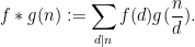
A key operation on arithmetic functions is that of Dirichlet convolution, which when given two arithmetic functions 
Thus for instance 


 = {\mathcal D}[f](s) {\mathcal D}[g](s), \ \ \ \ \ (3)](https://s0.wp.com/latex.php?latex=%5Cdisplaystyle+%7B%5Cmathcal+D%7D%5Bf+%2A+g%5D%28s%29+%3D+%7B%5Cmathcal+D%7D%5Bf%5D%28s%29+%7B%5Cmathcal+D%7D%5Bg%5D%28s%29%2C+%5C+%5C+%5C+%5C+%5C+%283%29&bg=ffffff&fg=000000&s=0&c=20201002)
at least when the real part of
 = - \frac{d}{ds} {\mathcal D}[f](s), \ \ \ \ \ (4)](https://s0.wp.com/latex.php?latex=%5Cdisplaystyle+%7B%5Cmathcal+D%7D%5BLf%5D%28s%29+%3D+-+%5Cfrac%7Bd%7D%7Bds%7D+%7B%5Cmathcal+D%7D%5Bf%5D%28s%29%2C+%5C+%5C+%5C+%5C+%5C+%284%29&bg=ffffff&fg=000000&s=0&c=20201002)
at least when the real part of ![{\zeta = {\mathcal D}[1]}](https://s0.wp.com/latex.php?latex=%7B%5Czeta+%3D+%7B%5Cmathcal+D%7D%5B1%5D%7D&bg=ffffff&fg=000000&s=0&c=20201002)
 = \zeta^2(s)](https://s0.wp.com/latex.php?latex=%5Cdisplaystyle+%7B%5Cmathcal+D%7D%5Bd_2%5D%28s%29+%3D+%5Czeta%5E2%28s%29&bg=ffffff&fg=000000&s=0&c=20201002)
 = - \zeta'(s)](https://s0.wp.com/latex.php?latex=%5Cdisplaystyle+%7B%5Cmathcal+D%7D%5BL%5D%28s%29+%3D+-+%5Czeta%27%28s%29+&bg=ffffff&fg=000000&s=0&c=20201002)
 = 1](https://s0.wp.com/latex.php?latex=%5Cdisplaystyle+%7B%5Cmathcal+D%7D%5B%5Cdelta%5D%28s%29+%3D+1&bg=ffffff&fg=000000&s=0&c=20201002)
 = \frac{1}{\zeta(s)}](https://s0.wp.com/latex.php?latex=%5Cdisplaystyle+%7B%5Cmathcal+D%7D%5B%5Cmu%5D%28s%29+%3D+%5Cfrac%7B1%7D%7B%5Czeta%28s%29%7D&bg=ffffff&fg=000000&s=0&c=20201002)
 = -\frac{\zeta'(s)}{\zeta(s)}.](https://s0.wp.com/latex.php?latex=%5Cdisplaystyle+%7B%5Cmathcal+D%7D%5B%5CLambda%5D%28s%29+%3D+-%5Cfrac%7B%5Czeta%27%28s%29%7D%7B%5Czeta%28s%29%7D.&bg=ffffff&fg=000000&s=0&c=20201002)
Much of the difficulty of multiplicative number theory can be traced back to the discrete nature of the natural numbers 


and similarly the analogue of (2) is

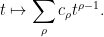
The analogue of the Dirichlet series is the Mellin-type transform
 := \int_1^\infty \frac{f(t)}{t^s}\ dt,](https://s0.wp.com/latex.php?latex=%5Cdisplaystyle+%7B%5Cmathcal+D%7D_%5Cinfty%5Bf%5D%28s%29+%3A%3D+%5Cint_1%5E%5Cinfty+%5Cfrac%7Bf%28t%29%7D%7Bt%5Es%7D%5C+dt%2C&bg=ffffff&fg=000000&s=0&c=20201002)
which will be well-defined at least if the real part of
For instance, the continuous analogue of the discrete constant function 


and

where 


 = \zeta(s) \approx \frac{1}{s-1} = {\mathcal D}_\infty[1_\infty](s)](https://s0.wp.com/latex.php?latex=%5Cdisplaystyle+%7B%5Cmathcal+D%7D%5B1%5D%28s%29+%3D+%5Czeta%28s%29+%5Capprox+%5Cfrac%7B1%7D%7Bs-1%7D+%3D+%7B%5Cmathcal+D%7D_%5Cinfty%5B1_%5Cinfty%5D%28s%29&bg=ffffff&fg=000000&s=0&c=20201002)
which reflects the fact that  = \frac{1}{s-1}}](https://s0.wp.com/latex.php?latex=%7B%7B%5Cmathcal+D%7D_%5Cinfty%5B1_%5Cinfty%5D%28s%29+%3D+%5Cfrac%7B1%7D%7Bs-1%7D%7D&bg=ffffff&fg=000000&s=0&c=20201002)
![{{\mathcal D}_\infty[1_\infty]}](https://s0.wp.com/latex.php?latex=%7B%7B%5Cmathcal+D%7D_%5Cinfty%5B1_%5Cinfty%5D%7D&bg=ffffff&fg=000000&s=0&c=20201002)
In a similar vein, the logarithm function 

of Stirling’s formula, or the Dirichlet series approximation
 = -\zeta'(s) \approx \frac{1}{(s-1)^2} = {\mathcal D}_\infty[L_\infty](s).](https://s0.wp.com/latex.php?latex=%5Cdisplaystyle+%7B%5Cmathcal+D%7D%5BL%5D%28s%29+%3D+-%5Czeta%27%28s%29+%5Capprox+%5Cfrac%7B1%7D%7B%28s-1%29%5E2%7D+%3D+%7B%5Cmathcal+D%7D_%5Cinfty%5BL_%5Cinfty%5D%28s%29.&bg=ffffff&fg=000000&s=0&c=20201002)
The continuous analogue of Dirichlet convolution is multiplicative convolution using the multiplicative Haar measure 
Thus for instance 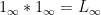
 = D_\infty[f_\infty](s) D_\infty[g_\infty](s)](https://s0.wp.com/latex.php?latex=%5Cdisplaystyle+D_%5Cinfty%5Bf_%5Cinfty+%2A_%5Cinfty+g_%5Cinfty%5D%28s%29+%3D+D_%5Cinfty%5Bf_%5Cinfty%5D%28s%29+D_%5Cinfty%5Bg_%5Cinfty%5D%28s%29&bg=ffffff&fg=000000&s=0&c=20201002)
of (3) whenever the real part of
 = -\frac{d}{ds} D_\infty[f_\infty](s) \ \ \ \ \ (5)](https://s0.wp.com/latex.php?latex=%5Cdisplaystyle+D_%5Cinfty%5BL_%5Cinfty+f_%5Cinfty%5D%28s%29+%3D+-%5Cfrac%7Bd%7D%7Bds%7D+D_%5Cinfty%5Bf_%5Cinfty%5D%28s%29+%5C+%5C+%5C+%5C+%5C+%285%29&bg=ffffff&fg=000000&s=0&c=20201002)
again assuming that the real part of
Direct calculation shows that for any complex number
](https://s0.wp.com/latex.php?latex=%5Cdisplaystyle+%5Cfrac%7B1%7D%7Bs-%5Crho%7D+%3D+D_%5Cinfty%5B+t+%5Cmapsto+t%5E%7B%5Crho-1%7D+%5D%28s%29&bg=ffffff&fg=000000&s=0&c=20201002)
(at least for the real part of
](https://s0.wp.com/latex.php?latex=%5Cdisplaystyle+%5Cfrac%7B1%7D%7B%28s-%5Crho%29%5Ek%7D+%3D+D_%5Cinfty%5B+t+%5Cmapsto+%5Cfrac%7B1%7D%7B%28k-1%29%21%7D+t%5E%7B%5Crho-1%7D+%5Clog%5E%7Bk-1%7D+t+%5D%28s%29&bg=ffffff&fg=000000&s=0&c=20201002)
for any natural number }](https://s0.wp.com/latex.php?latex=%7BD%5Bf%5D%28s%29%7D&bg=ffffff&fg=000000&s=0&c=20201002)

 \approx \sum_\rho \frac{c_\rho}{(s-\rho)^{k_\rho}}](https://s0.wp.com/latex.php?latex=%5Cdisplaystyle+D%5Bf%5D%28s%29+%5Capprox+%5Csum_%5Crho+%5Cfrac%7Bc_%5Crho%7D%7B%28s-%5Crho%29%5E%7Bk_%5Crho%7D%7D&bg=ffffff&fg=000000&s=0&c=20201002)
for some set 


In particular, if we only have simple poles,
 \approx \sum_\rho \frac{c_\rho}{s-\rho}](https://s0.wp.com/latex.php?latex=%5Cdisplaystyle+D%5Bf%5D%28s%29+%5Capprox+%5Csum_%5Crho+%5Cfrac%7Bc_%5Crho%7D%7Bs-%5Crho%7D&bg=ffffff&fg=000000&s=0&c=20201002)
then we expect to have
Integrating this from

for the summatory function, and similarly
with the convention that 


For instance, using the more refined approximation
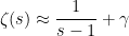
to the zeta function near
 = \zeta^2(s) \approx \frac{1}{(s-1)^2} + \frac{2 \gamma}{s-1}](https://s0.wp.com/latex.php?latex=%5Cdisplaystyle+%7B%5Cmathcal+D%7D%5Bd_2%5D%28s%29+%3D+%5Czeta%5E2%28s%29+%5Capprox+%5Cfrac%7B1%7D%7B%28s-1%29%5E2%7D+%2B+%5Cfrac%7B2+%5Cgamma%7D%7Bs-1%7D&bg=ffffff&fg=000000&s=0&c=20201002)
we would expect that

and thus for instance

which matches what one actually gets from the Dirichlet hyperbola method (see e.g. equation (44) of this previous post).
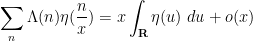
Or, noting that 


 = -\frac{\zeta'(s)}{\zeta(s)} \approx \frac{1}{s-1} - \sum_\rho \frac{1}{s-\rho}](https://s0.wp.com/latex.php?latex=%5Cdisplaystyle+%7B%5Cmathcal+D%7D%5B%5CLambda%5D%28s%29+%3D+-%5Cfrac%7B%5Czeta%27%28s%29%7D%7B%5Czeta%28s%29%7D+%5Capprox+%5Cfrac%7B1%7D%7Bs-1%7D+-+%5Csum_%5Crho+%5Cfrac%7B1%7D%7Bs-%5Crho%7D&bg=ffffff&fg=000000&s=0&c=20201002)
suggesting that
leading for instance to the summatory approximation

which is a heuristic form of the Riemann-von Mangoldt explicit formula (see Exercise 45 of these notes for a rigorous version of this formula).
Exercise 1 Go through some of the other explicit formulae listed at this Wikipedia page and give heuristic justifications for them (up to some lower order terms) by similar calculations to those given above.
Given the “adelic” perspective on number theory, I wonder if there are also 


In analytic number theory, there is a well known analogy between the prime factorisation of a large integer, and the cycle decomposition of a large permutation; this analogy is central to the topic of “anatomy of the integers”, as discussed for instance in this survey article of Granville. Consider for instance the following two parallel lists of facts (stated somewhat informally). Firstly, some facts about the prime factorisation of large integers:
- Every positive integer
into (not necessarily distinct) primes
, which is unique up to rearrangement. Taking logarithms, we obtain a partition
of
.
- (Prime number theorem) A randomly selected integer
will be prime with probability
when
is large.
- If
is a randomly selected prime factor of
(with each index
being chosen with probability
), then
is approximately uniformly distributed between
. (See Proposition 9 of this previous blog post.)
- The set of real numbers
arising from the prime factorisation
. (See the previously mentioned blog post for a definition of the Poisson-Dirichlet process, and a proof of this claim.)


Now for the facts about the cycle decomposition of large permutations:
- Every permutation
has a cycle decomposition
into disjoint cycles
, which is unique up to rearrangement, and where we count each fixed point of
is the length of the cycle
, we obtain a partition
of
- (Prime number theorem for permutations) A randomly selected permutation of
will be an
. (This was noted in this previous blog post.)
- If
), then
. (See Proposition 8 of this blog post.)
- The set of real numbers
arising from the cycle decomposition
of a random permutation


See this previous blog post (or the aforementioned article of Granville, or the Notices article of Arratia, Barbour, and Tavaré) for further exploration of the analogy between prime factorisation of integers and cycle decomposition of permutations.
There is however something unsatisfying about the analogy, in that it is not clear why there should be such a kinship between integer prime factorisation and permutation cycle decomposition. It turns out that the situation is clarified if one uses another fundamental analogy in number theory, namely the analogy between integers and polynomials ![{P \in {\mathbf F}_q[T]}](https://s0.wp.com/latex.php?latex=%7BP+%5Cin+%7B%5Cmathbf+F%7D_q%5BT%5D%7D&bg=ffffff&fg=000000&s=0&c=20201002)


- Every monic polynomial
has a factorisation
into irreducible monic polynomials
, which is unique up to rearrangement. Taking degrees, we obtain a partition
of
.
- (Prime number theorem for polynomials) A randomly selected monic polynomial
when
- If
is a random irreducible factor of
(with each
), then
is approximately uniformly distributed in
- The set of real numbers
arising from the factorisation


The above list of facts addressed the large ![{{\mathbf F}_q[T]}](https://s0.wp.com/latex.php?latex=%7B%7B%5Cmathbf+F%7D_q%5BT%5D%7D&bg=ffffff&fg=000000&s=0&c=20201002)

The large
Theorem 1 (Prime number theorem) The probability that a random monic polynomial
in the limit where
Proof: There are 


Remark 2 The above argument and inclusion-exclusion in fact gives the well known exact formula
for the number of irreducible monic polynomials of degree
Now we can give a precise connection between the cycle distribution of a random permutation, and (the large
Theorem 3 The partition
of a random monic polynomial
of degree
of a random permutation
of length
We can quickly prove this theorem as follows. We first need a basic fact:
Lemma 4 (Most polynomials square-free in large
when
of degree
will be coprime with probability
Proof: For any polynomial 


Now we can prove the theorem. Elementary combinatorics tells us that the probability of a random permutation 


since there are 

which simplifies to

and the claim follows.
This was a fairly short calculation, but it still doesn’t quite explain why there is such a link between the cycle decomposition 


I recently found (after some discussions with Ben Green) what I feel to be a satisfying conceptual (as opposed to computational) explanation of this link, which I will place below the fold.
In the previous set of notes, we saw how zero-density theorems for the Riemann zeta function, when combined with the zero-free region of Vinogradov and Korobov, could be used to obtain prime number theorems in short intervals. It turns out that a more sophisticated version of this type of argument also works to obtain prime number theorems in arithmetic progressions, in particular establishing the celebrated theorem of Linnik:
Theorem 1 (Linnik’s theorem) Let
be a primitive residue class. Then
.
In fact it is known that one can find a prime 

We will not aim to obtain the optimal exponents for Linnik’s theorem here, and follow the treatment in Chapter 18 of Iwaniec and Kowalski. We will in fact establish the following more quantitative result (a special case of a more powerful theorem of Gallagher), which splits into two cases, depending on whether there is an exceptional zero or not:
Theorem 2 (Quantitative Linnik theorem) Let
. For any
denote the quantity
Assume that
for some sufficiently large
.
- (i) (No exceptional zero) If all the real zeroes
of
-functions
of real characters
, then
for all
.
- (ii) (Exceptional zero) If there is a zero
of a real character
of modulus
for some sufficiently small
, then
for all
The implied constants here are effective.


Note from the Landau-Page theorem (Exercise 54 from Notes 2) that at most one exceptional zero exists (if 

Exercise 3 Assuming Theorem 2, and assuming
when there is no exceptional zero, and
when there is an exceptional zero

Remark 4 The Brun-Titchmarsh theorem (Exercise 33 from Notes 4), in the sharp form of Montgomery and Vaughan, gives that
for any primitive residue class
. This is (barely) consistent with the estimate (1). Any lowering of the coefficient
in the Brun-Titchmarsh inequality (with reasonable error terms), in the regime when

Theorem 2 is deduced in turn from facts about the distribution of zeroes of
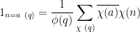
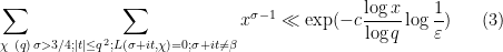
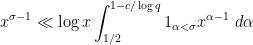
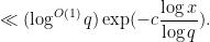
Exercise 5 (Log-free truncated explicit formula) With the hypotheses as above, show that
for any non-principal character
, except that there is a factor of
in the error term instead of
when
. To get rid of the final factor of
. If one replaces this crude bound by more sophisticated tools such as the Brun-Titchmarsh inequality, one will be able to remove the factor of

Using the Fourier inversion formula
(see Theorem 69 of Notes 1), we thus have
and so it suffices by the triangle inequality (bounding 

when no exceptional zero is present, and
when an exceptional zero is present.
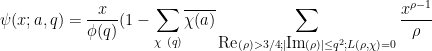
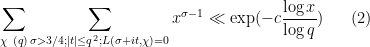
To handle the former case (2), one uses two facts about zeroes. The first is the classical zero-free region (Proposition 51 from Notes 2), which we reproduce in our context here:
Proposition 6 (Classical zero-free region) Let
. Apart from a potential exceptional zero
of
are such that
for some absolute constant

Using this zero-free region, we have
whenever

where we recall that 


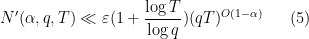
In Exercise 25 of Notes 6, the grand density estimate

is proven. If one inserts this bound into the above expression, one obtains a bound for (2) which is of the form
Unfortunately this is off from what we need by a factor of 


Theorem 7 (Log-free grand density estimate) For any
and
, one has
The implied constants are effective.

We prove this estimate below the fold. The proof follows the methods of the previous section, but one inserts various sieve weights to restrict sums over natural numbers to essentially become sums over “almost primes”, as this turns out to remove the logarithmic losses. (More generally, the trick of restricting to almost primes by inserting suitable sieve weights is quite useful for avoiding any unnecessary losses of logarithmic factors in analytic number theory estimates.)
Now we turn to the case when there is an exceptional zero (3). The argument used to prove (2) applies here also, but does not gain the factor of 
Theorem 9 (Deuring-Heilbronn repulsion phenomenon) Suppose
In other words, the exceptional zero enlarges the classical zero-free region by a factor of

Exercise 10 Use Theorem 7 and Theorem 9 to complete the proof of (3), and thus Linnik’s theorem.
Exercise 11 Use Theorem 9 to give an alternate proof of (Tatuzawa’s version of) Siegel’s theorem (Theorem 62 of Notes 2). (Hint: if two characters have different moduli, then they can be made to have the same modulus by multiplying by suitable principal characters.)
Theorem 9 is proven by similar methods to that of Theorem 7, the basic idea being to insert a further weight of 
with effective implied constants for any 


Remark 12 There are a number of alternate ways to derive the results in this set of notes, for instance using the Turan power sums method which is based on studying derivatives such as
for
and large


Remark 13 When one optimises all the exponents, it turns out that the exponent in Linnik’s theorem is extremely good in the presence of an exceptional zero – indeed Friedlander and Iwaniec showed can even get a bound of the form
for some
In the previous set of notes, we studied upper bounds on sums such as 

![{[T,2T]}](https://s0.wp.com/latex.php?latex=%7B%5BT%2C2T%5D%7D&bg=ffffff&fg=000000&s=0&c=20201002)


However, it turns out that one can get much better bounds if one settles for estimating sums such as 
Our main application of the large value theorems for Dirichlet polynomials will be to control the number of zeroes of the Riemann zeta function 


In the next set of notes we will use refined versions of these theorems to establish Linnik’s theorem on the least prime in an arithmetic progression.
Our presentation here is broadly based on Chapters 9 and 10 in Iwaniec and Kowalski, who give a number of more sophisticated large value theorems than the ones discussed here.
The prime number theorem can be expressed as the assertion

as

is the von Mangoldt function. It is a basic result in analytic number theory, but requires a bit of effort to prove. One “elementary” proof of this theorem proceeds through the Selberg symmetry formula
where the second von Mangoldt function 


(We are avoiding the use of the 

suffices.
In this post I would like to record a somewhat “soft analysis” reformulation of the elementary proof of the prime number theorem in terms of Banach algebras, and specifically in Banach algebra structures on (completions of) the space 

This soft argument does not easily give any quantitative decay rate in the prime number theorem, but by the same token it avoids many of the quantitative calculations in the traditional proofs of this theorem. Ultimately, the key “soft analysis” fact used is the spectral radius formula

for any element 


The connection between prime numbers and Banach algebras is given by the following consequence of the Selberg symmetry formula.
Theorem 1 (Construction of a Banach algebra norm) For any
, let
denote the quantity
Then
is a seminorm on
for all
for all
.


We prove this theorem below the fold. The prime number theorem then follows from Theorem 1 and the following two assertions. The first is an application of the spectral radius formula (6) and some basic Fourier analysis (in particular, the observation that
Theorem 2 (Non-trivial Banach algebras with many local units have non-trivial spectrum) Let
such that
for all
. In particular, by (7), one has
whenever
is a non-negative function.


The second is a consequence of the Selberg symmetry formula and the fact that 

Theorem 3 (Breaking the parity barrier) Let

Assuming Theorems 1, 2, 3, we may now quickly establish the prime number theorem as follows. Theorem 2 and Theorem 3 imply that the seminorm

as 


as
as
The same argument also yields the prime number theorem in arithmetic progressions, or equivalently that

for any fixed Dirichlet character 
One of the most basic methods in additive number theory is the Hardy-Littlewood circle method. This method is based on expressing a quantity of interest to additive number theory, such as the number of representations 


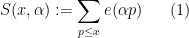
where the sum here ranges over all primes up to 


The strategy is then to obtain sufficiently accurate bounds on exponential sums such as 


Remark 1 In practice, it can be more efficient to work with smoother sums than the partial sum (1), for instance by replacing the cutoff
for a suitable choice of cutoff function
In many cases, it turns out that one can get fairly precise evaluations on sums such as 
and the prime number theorem in residue classes modulo
when 


In the minor arc case when 

for “typical” minor arc
which is consistent with (though weaker than) the above heuristic. In practice, though, we are unable to rigorously establish bounds anywhere near as strong as (3); upper bounds such as 
Because one only expects to have upper bounds on 


Despite this handicap, though, it is still possible to get enough bounds on both the major and minor arc contributions of integrals such as (2) to obtain non-trivial lower bounds on quantities such as 
However, I (and many other analytic number theorists) are considerably more skeptical that the circle method can be applied to the even Goldbach problem of representing a large even number 

for sufficiently large 


that goes to infinity as 

In principle, one can achieve either of these two objectives by a sufficiently fine level of control on the exponential sums 
Of course, this would not qualify as a genuine application of the circle method by any reasonable measure. One can then ask the more refined question of whether one could hope to get non-trivial lower bounds on 

- (i) For “binary” problems such as computing (5), (6), the contribution of the minor arcs potentially dominates that of the major arcs (if all one is given about the minor arc sums is magnitude information), in contrast to “ternary” problems such as computing (2), in which it is the major arc contribution which is absolutely dominant.
- (ii) Upper and lower bounds on the magnitude of
or better); but
- (iii) obtaining such tight bounds is a problem of comparable difficulty to the original binary problems.
I will provide some justification for these conclusions below the fold; they are reasonably well known “folklore” to many researchers in the field, but it seems that they are rarely made explicit in the literature (in part because these arguments are, by their nature, heuristic instead of rigorous) and I have been asked about them from time to time, so I decided to try to write them down here.
In view of the above conclusions, it seems that the best one can hope to do by using the circle method for the twin prime or even Goldbach problems is to reformulate such problems into a statement of roughly comparable difficulty to the original problem, even if one assumes powerful conjectures such as the Generalised Riemann Hypothesis (which lets one make very precise control on major arc exponential sums, but not on minor arc ones). These are not rigorous conclusions – after all, we have already seen that one can always artifically insert the circle method into any viable approach on these problems – but they do strongly suggest that one needs a method other than the circle method in order to fully solve either of these two problems. I do not know what such a method would be, though I can give some heuristic objections to some of the other popular methods used in additive number theory (such as sieve methods, or more recently the use of inverse theorems); this will be done at the end of this post.
A fundamental problem in analytic number theory is to understand the distribution of the prime numbers 


The most important result in this subject is the prime number theorem, which asserts that the number of prime numbers less than a large number 

Here, of course,
It is not hard to see (e.g. by summation by parts) that this is equivalent to the asymptotic
for the von Mangoldt function (the key point being that the squares, cubes, etc. of primes give a negligible contribution, so 


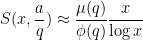
The prime number theorem has several important generalisations (for instance, there are analogues for other number fields such as the Chebotarev density theorem). One of the more elementary such generalisations is the prime number theorem in arithmetic progressions, which asserts that for fixed 


(Of course, if 


As before, one can rewrite the prime number theorem in arithmetic progressions in terms of the von Mangoldt function as the equivalent form
Philosophically, one of the main reasons why it is so hard to control the distribution of the primes is that we do not currently have too many tools with which one can rule out “conspiracies” between the primes, in which the primes (or the von Mangoldt function) decide to correlate with some structured object (and in particular, with a totally multiplicative function) which then visibly distorts the distribution of the primes. For instance, one could imagine a scenario in which the probability that a randomly chosen large integer 


In the above scenario, the primality of a large integer 


An especially difficult scenario to eliminate is that of real characters, such as the Kronecker symbol 
It is difficult to prove that no conspiracy between the primes exist. However, it is not entirely impossible, because we have been able to exploit two important phenomena. The first is that there is often a “all or nothing dichotomy” (somewhat resembling the zero-one laws in probability) regarding conspiracies: in the asymptotic limit, the primes can either conspire totally (or more precisely, anti-conspire totally) with a multiplicative function, or fail to conspire at all, but there is no middle ground. (In the language of Dirichlet series, this is reflected in the fact that zeroes of a meromorphic function can have order
But now one can use the second important phenomenon, which is that because of symmetries, one type of conspiracy can lead to another. For instance, because the von Mangoldt function is real-valued rather than complex-valued, we have conjugation symmetry; if the primes correlate with, say, 

As mentioned previously in passing, these phenomena are usually presented using the language of Dirichlet series and complex analysis. This is a very slick and powerful way to do things, but I would like here to present the elementary approach to the same topics, which is slightly weaker but which I find to also be very instructive. (However, I will not be too dogmatic about keeping things elementary, if this comes at the expense of obscuring the key ideas; in particular, I will rely on multiplicative Fourier analysis (both at
The material here is closely related to the theory of pretentious characters developed by Granville and Soundararajan, as well as an earlier paper of Granville on elementary proofs of the prime number theorem in arithmetic progressions.
Atle Selberg, who made immense and fundamental contributions to analytic number theory and related areas of mathematics, died last Monday, aged 90.
Selberg’s early work was focused on the study of the Riemann zeta function 

In working on the zeta function, Selberg developed two powerful tools which are still used routinely in analytic number theory today. The first is the method of mollifiers to smooth out the magnitude oscillations of the zeta function, making the (more interesting) phase oscillation more visible. The second was the method of the Selberg 
For all of these achievements, Selberg was awarded the Fields Medal in 1950. Around that time, Selberg and Erdős also produced the first elementary proof of the prime number theorem. A key ingredient here was the Selberg symmetry formula, which is an elementary analogue of the prime number theorem for almost primes.
But perhaps Selberg’s greatest contribution to mathematics was his discovery of the Selberg trace formula, which is a non-abelian generalisation of the Poisson summation formula, and which led to many further deep connections between representation theory and number theory, and in particular being one of the main inspirations for the Langlands program, which in turn has had an impact on many different parts of mathematics (for instance, it plays a role in Wiles’ proof of Fermat’s last theorem). For an introduction to the trace formula, its history, and its impact, I recommend the survey article of Arthur.
Other major contributions of Selberg include the Rankin-Selberg theory connecting Artin L-functions from representation theory to the integrals of automorphic forms (very much in the spirit of the Langlands program), and the Chowla-Selberg formula relating the Gamma function at rational values to the periods of elliptic curves with complex multiplication. He also made an influential conjecture on the spectral gap of the Laplacian on quotients of 

Recent Comments