
You are currently browsing the tag archive for the ‘Cayley graphs’ tag.
The wave equation is usually expressed in the form

where 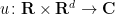


which we can rewrite using integration by parts and the 


A key feature of the wave equation is finite speed of propagation: if, at time 


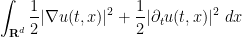
and observing (after some integration by parts and differentiation under the integral sign) that it is non-increasing in time, non-negative, and vanishing at time
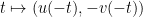
The wave equation is second order in time, but one can turn it into a first order system by working with the pair 


and the conserved energy is now

Finite speed of propagation then tells us that if 


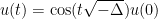
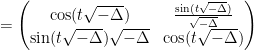
If one has an eigenfunction

of the Laplacian, then we have the explicit solutions


of the wave equation, which formally can be used to construct all other solutions via the principle of superposition.
When one has vanishing initial velocity 
and the propagator 

One can view 

which is unitary with respect to the energy form (1), and is the fundamental solution to the wave equation in the sense that

Viewing the contraction 
It turns out (as I learned from Yuval Peres) that there is a useful discrete analogue of the wave equation (and of all of the above facts), in which the time variable 


where 


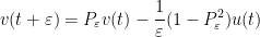
where 


Assuming

This energy is positive semi-definite if

to the operator

to (3), and (in principle at least) this generates all other solutions via the principle of superposition.
Finite speed of propagation is a lot easier in the discrete setting, though one has to offset the support of the “velocity” field 


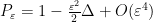
The fundamental solution 

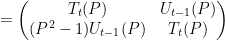
where 


and

In particular, 


As before, 


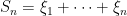
One nice application of all this formalism, which I learned from Yuval Peres, is the Varopoulos-Carne inequality:
Theorem 1 (Varopoulos-Carne inequality) Let
, and let
be vertices in
lands at
at time
is at most
, where
is the graph distance.
This general inequality is quite sharp, as one can see using the standard Cayley graph on the integers 
Proof: Let 

for any 


where 


where we are now using the energy form (4). We can write

where 


By finite speed of propagation, the inner product here vanishes if 


and the claim now follows from the Chernoff inequality.

This inequality has many applications, particularly with regards to relating the entropy, mixing time, and concentration of random walks with volume growth of balls; see this text of Lyons and Peres for some examples.
For sake of comparison, here is a continuous counterpart to the Varopoulos-Carne inequality:
Theorem 2 (Continuous Varopoulos-Carne inequality) Let
, and let
be supported on compact sets
respectively. Then
where
is the Euclidean distance between
and

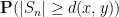
Proof: By Fourier inversion one has
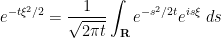
for any real 

By finite speed of propagation, the inner product 


Bounding 

Observe that the argument is quite general and can be applied for instance to other Riemannian manifolds than
This is a sequel to my previous blog post “Cayley graphs and the geometry of groups“. In that post, the concept of a Cayley graph of a group
Throughout this post, we fix a single group 
In the previous post, we drew the entire Cayley graph of a group 


Figure 1.
One usually does not work with the complete Cayley graph 
Cayley graphs are left-invariant: for any 


Figure 2.
This is analogous to how, in undergraduate mathematics and physics, vectors in Euclidean space are often depicted as arrows of a given magnitude and direction, with the initial and final points of this arrow being of secondary importance only. (Indeed, this depiction of vectors in a vector space can be viewed as an abelian special case of the more general depiction of group elements used in this post.)
Let us define a diagram to be a finite directed graph 


We will however omit the identity loops in our diagrams in order to reduce clutter.
We make the obvious remark that any directed edge in a diagram can be coloured by at most one group element 


Remark 1 One can also interpret these diagrams as commutative diagrams in a category in which all the objects are copies of
Just as vector addition can be expressed via concatenation of arrows, group multiplication can be described by concatenation of directed edges. Indeed, for any 

 Figure 4.
In a similar spirit, inversion is described by the following diagram:

Figure 5.
We make the pedantic remark though that we do not consider a 
A fundamental operation for us will be that of gluing two diagrams together.
Lemma 1 ((Labeled) gluing) Let
be two diagrams of a given group
of the two diagrams connects all of
(i.e. any two elements of
). Then the union
is also a diagram of
Proof: By hypothesis, we have graph homomorphisms 


The above lemma required one to specify the label the vertices of 


For instance, if a diagram

Figure 6.
One can use glued diagrams to demonstrate various basic group-theoretic identities. For instance, by gluing together two copies of the triangular diagram in Figure 4 to create the glued diagram

Figure 7.
and then filling in two more triangles, we obtain a tetrahedral diagram that demonstrates the associative law 

Figure 8.
Similarly, by gluing together two copies of Figure 4 with three copies of Figure 5 in an appropriate order, we can demonstrate the Abel identity 

Figure 9.
In addition to gluing, we will also use the trivial operation of erasing: if
If two group elements

Figure 10.
In general, of course, two arbitrary group elements 


Figure 11.
By appropriate gluing and filling, this can be used to demonstrate the homomorphism properties of a conjugation map 

Figure 12.

Figure 13.
Another way to replace the parallelogram in Figure 10 is to introduce the commutator ![{[g,h] := g^{-1}h^{-1}gh}](https://s0.wp.com/latex.php?latex=%7B%5Bg%2Ch%5D+%3A%3D+g%5E%7B-1%7Dh%5E%7B-1%7Dgh%7D&bg=ffffff&fg=000000&s=0&c=20201002)

Figure 14.
We will tend to depict commutator edges as being somewhat shorter than the edges generating that commutator, reflecting a “perturbative” or “nilpotent” philosophy. (Of course, to fully reflect a nilpotent perspective, one should orient commutator edges in a different dimension from their generating edges, but of course the diagrams drawn here do not have enough dimensions to display this perspective easily.) We will also be adopting a “Lie” perspective of interpreting groups as behaving like perturbations of vector spaces, in particular by trying to draw all edges of the same colour as being approximately (though not perfectly) parallel to each other (and with approximately the same length).
Gluing the above pentagon with the conjugation parallelogram and erasing some edges, we discover a “commutator-conjugate” triangle, describing the basic identity ![{g^h = g [g,h]}](https://s0.wp.com/latex.php?latex=%7Bg%5Eh+%3D+g+%5Bg%2Ch%5D%7D&bg=ffffff&fg=000000&s=0&c=20201002)

Figure 15.
Other gluings can also give the basic relations between commutators and conjugates. For instance, by gluing the pentagon in Figure 14 with its reflection, we see that ![{[g,h] = [h,g]^{-1}}](https://s0.wp.com/latex.php?latex=%7B%5Bg%2Ch%5D+%3D+%5Bh%2Cg%5D%5E%7B-1%7D%7D&bg=ffffff&fg=000000&s=0&c=20201002)
![{[h,g^{-1}] = [g,h]^{g^{-1}}}](https://s0.wp.com/latex.php?latex=%7B%5Bh%2Cg%5E%7B-1%7D%5D+%3D+%5Bg%2Ch%5D%5E%7Bg%5E%7B-1%7D%7D%7D&bg=ffffff&fg=000000&s=0&c=20201002)

Figure 16.
while this figure demonstrates that ![{[g,hk] = [g,k] [g,h]^k}](https://s0.wp.com/latex.php?latex=%7B%5Bg%2Chk%5D+%3D+%5Bg%2Ck%5D+%5Bg%2Ch%5D%5Ek%7D&bg=ffffff&fg=000000&s=0&c=20201002)

Figure 17.
Now we turn to a more sophisticated identity, the Hall-Witt identity
![\displaystyle [[g,h],k^g] [[k,g],h^k] [[h,k],g^h] = 1,](https://s0.wp.com/latex.php?latex=%5Cdisplaystyle+%5B%5Bg%2Ch%5D%2Ck%5Eg%5D+%5B%5Bk%2Cg%5D%2Ch%5Ek%5D+%5B%5Bh%2Ck%5D%2Cg%5Eh%5D+%3D+1%2C&bg=ffffff&fg=000000&s=0&c=20201002)
which is the fully noncommutative version of the more well-known Jacobi identity for Lie algebras.
The full diagram for the Hall-Witt identity resembles a slightly truncated parallelopiped. Drawing this truncated paralleopiped in full would result in a rather complicated looking diagram, so I will instead display three components of this diagram separately, and leave it to the reader to mentally glue these three components back to form the full parallelopiped. The first component of the diagram is formed by gluing together three pentagons from Figure 14, and looks like this:
 Figure 18.
This should be thought of as the “back” of the truncated parallelopiped needed to establish the Hall-Witt identity.
While it is not needed for proving the Hall-Witt identity, we also observe for future reference that we may also glue in some distorted parallelograms and obtain a slightly more complicated diagram:

Figure 19.
To form the second component, let us now erase all interior components of Figure 18 or Figure 19:

Figure 20.
Then we fill in three distorted parallelograms:

Figure 21.
This is the second component, and is the “front” of the truncated praallelopiped, minus the portions exposed by the truncation.
Finally, we turn to the third component. We begin by erasing the outer edges from the second component in Figure 21:

Figure 22.
We glue in three copies of the commutator-conjugate triangle from Figure 15:

Figure 23.
But now we observe that we can fill in three pentagons, and obtain a small triangle with edges ![{[[g,h],k^g] [[k,g],h^k] [[h,k],g^h]}](https://s0.wp.com/latex.php?latex=%7B%5B%5Bg%2Ch%5D%2Ck%5Eg%5D+%5B%5Bk%2Cg%5D%2Ch%5Ek%5D+%5B%5Bh%2Ck%5D%2Cg%5Eh%5D%7D&bg=ffffff&fg=000000&s=0&c=20201002)

Figure 24.
Erasing everything except this triangle gives the Hall-Witt identity. Alternatively, one can glue together Figures 18, 21, and 24 to obtain a truncated parallelopiped which one can view as a geometric representation of the proof of the Hall-Witt identity.
Among other things, I found these diagrams to be useful to visualise group cohomology; I give a simple example of this below, developing an analogue of the Hall-Witt identity for 
In this final set of course notes, we discuss how (a generalisation of) the expansion results obtained in the preceding notes can be used for some number-theoretic applications, and in particular to locate almost primes inside orbits of thin groups, following the work of Bourgain, Gamburd, and Sarnak. We will not attempt here to obtain the sharpest or most general results in this direction, but instead focus on the simplest instances of these results which are still illustrative of the ideas involved.
One of the basic general problems in analytic number theory is to locate tuples of primes of a certain form; for instance, the famous (and still unsolved) twin prime conjecture asserts that there are infinitely many pairs 


More generally, given some explicit subset 


At this level of generality, this problem is impossibly difficult. Indeed, even the much simpler problem of deciding whether the set 


Even in this simpler setting, the question of determining whether an orbit 


On the other hand, much more is known if one is willing to replace the primes by the larger set of almost primes – integers with a small number of prime factors (counting multiplicity). Specifically, for any 


The main tool that allows one to count almost primes in orbits is sieve theory. The reason for this lies in the simple observation that in order to ensure that an integer 
The most basic sieve of this form is the sieve of Eratosthenes, which when combined with the inclusion-exclusion principle gives the Legendre sieve (or exact sieve), which gives an exact formula for quantities such as the number 

Very roughly speaking, the end result of sieve theory is that excepting some degenerate and “exponentially thin” settings (such as those associated with the Mersenne primes), all the orbits which are expected to have a large number of primes, can be proven to at least have a large number of
Theorem 1 (Bourgain-Gamburd-Sarnak) Let
which is not virtually solvable. Let
be a polynomial with integer coefficients obeying the following primitivity condition: for any positive integer
, there exists
such that
is coprime to
with
This is not the strongest version of the Bourgain-Gamburd-Sarnak theorem, but it captures the general flavour of their results. Note that the theorem immediately implies an analogous result for orbits 


By specialising to the polynomial 
It turns out that to prove Theorem 1, the Cayley expansion results in 

In the previous set of notes we introduced the notion of expansion in arbitrary 
Definition 1 (Cayley graph) Let
be a finite subset of
whenever
) and does not contain the identity
, thus each vertex
is connected to the
elements
for
Example 2 The graph in Exercise 3 of Notes 1 is the Cayley graph on
with generators
.
Remark 3 We call the above Cayley graphs right-invariant because every right translation
on
rather than
, so we may without loss of generality restrict our attention throughout to left Cayley graphs.
Remark 4 For minor technical reasons, it will be convenient later on to allow
For the purposes of building expander families, we would of course want the underlying group
We will also sometimes consider a generalisation of a Cayley graph, known as a Schreier graph:
Definition 5 (Schreier graph) Let
, thus there is a map
from
to
and
for all
and
. Let
for all
for all distinct
and
is defined to be the graph with vertex set
.
Example 6 Every Cayley graph
, using the obvious left-action of
permutations
that were studied in the previous set of notes is also a Schreier graph provided that
for all distinct
, with the underlying group being the permutation group
in the obvious manner), and
.
Exercise 7 If
. (Hint: you may assume without proof Petersen’s 2-factor theorem, which asserts that every
We return now to Cayley graphs. It is easy to characterise qualitative expansion properties of Cayley graphs:
Exercise 8 (Qualitative expansion) Let
- (i) Show that
- (ii) Show that
We will however be interested in more quantitative expansion properties, in which the expansion constant 
One can analyse the expansion of Cayley graphs in a number of ways. For instance, by taking the edge expansion viewpoint, one can study Cayley graphs combinatorially, using the product set operation

of subsets of
Exercise 9 (Combinatorial description of expansion) Let
independent of
for all sufficiently large
of
with
.
One can also give a combinatorial description of two-sided expansion, but it is more complicated and we will not use it here.
Exercise 10 (Abelian groups do not expand) Let
). (Hint: assume for contradiction that
, and show by two different arguments that
grows at least exponentially in
and also at most polynomially in
The left-invariant nature of Cayley graphs also suggests that such graphs can be profitably analysed using some sort of Fourier analysis; as the underlying symmetry group is not necessarily abelian, one should use the Fourier analysis of non-abelian groups, which is better known as (unitary) representation theory. The Fourier-analytic nature of Cayley graphs can be highlighted by recalling the operation of convolution of two functions 

This convolution operation is bilinear and associative (at least when one imposes a suitable decay condition on the functions, such as compact support), but is not commutative unless 


where 

where 


whenever

whenever
We remark that the above spectral definition of expansion can be easily extended to symmetric sets 

obeys either (2) or (3).
We saw in the last set of notes that expansion can be characterised in terms of random walks. One can of course specialise this characterisation to the Cayley graph case:
Exercise 11 (Random walk description of expansion) Let
be the associated probability density functions. Let
be a constant.
- Show that the
such that for all sufficiently large
for some
, where
denotes the convolution of
- Show that the
for some
In this set of notes, we will connect expansion of Cayley graphs to an important property of certain infinite groups, known as Kazhdan’s property (T) (or property (T) for short). In 1973, Margulis exploited this property to create the first known explicit and deterministic examples of expanding Cayley graphs. As it turns out, property (T) is somewhat overpowered for this purpose; in particular, we now know that there are many families of Cayley graphs for which the associated infinite group does not obey property (T) (or weaker variants of this property, such as property 
The material here is based in part on this recent text on property (T) by Bekka, de la Harpe, and Valette (available online here).
Read the rest of this entry »
In most undergraduate courses, groups are first introduced as a primarily algebraic concept – a set equipped with a number of algebraic operations (group multiplication, multiplicative inverse, and multiplicative identity) and obeying a number of rules of algebra (most notably the associative law). It is only somewhat later that one learns that groups are not solely an algebraic object, but can also be equipped with the structure of a manifold (giving rise to Lie groups) or a topological space (giving rise to topological groups). (See also this post for a number of other ways to think about groups.)
Another important way to enrich the structure of a group 


One way to visualise the geometry of a generated group is to look at the (labeled) Cayley colour graph of the generated group
For instance, the Cayley graph of the cyclic group 


while the Cayley graph of the same group but with the generators 

We can thus see that the same group can have somewhat different geometry if one changes the set of generators. For instance, in a large cyclic group 
Cayley graphs have three distinguishing properties:
- (Regularity) For each colour
- (Connectedness) The graph is connected.
- (Homogeneity) For every pair of vertices
It is easy to verify that a directed coloured graph is a Cayley graph (up to relabeling) if and only if it obeys the above three properties. Indeed, given a graph 


From the above equivalence, we see that we do not really need the vertex labels on the Cayley graph in order to describe a generated group, and so we will now drop these labels and work solely with unlabeled Cayley graphs, in which the vertex set is not already identified with the group. As we saw above, one just needs to designate a marked vertex of the graph as the “identity” or “origin” in order to turn an unlabeled Cayley graph into a labeled Cayley graph; but from homogeneity we see that all vertices of an unlabeled Cayley graph “look the same” and there is no canonical preference for choosing one vertex as the identity over another. I prefer here to keep the graphs unlabeled to emphasise the homogeneous nature of the graph.
It is instructive to revisit the basic concepts of group theory using the language of (unlabeled) Cayley graphs, and to see how geometric many of these concepts are. In order to facilitate the drawing of pictures, I work here only with small finite groups (or Cayley graphs), but the discussion certainly is applicable to large or infinite groups (or Cayley graphs) also.
For instance, in this setting, the concept of abelianness is analogous to that of a flat (zero-curvature) geometry: given any two colours 


is not abelian.
A subgroup 


We saw that a subgroup 


Note, though, that the structure group of this connection is not simply 


over the field 


Note how close this group is to being abelian; more generally, one can think of nilpotent groups as being a slight perturbation of abelian groups.
In the case of 


This is a 
Even when one has a splitting, the bundle need not be completely trivial, because the bundle is not principal, and the connection can still twist the fibres around. For instance, 


the red fibre
Emmanuel Breuillard, Ben Green, and I have just uploaded to the arXiv our paper “Approximate subgroups of linear groups“, submitted to GAFA. This paper contains (the first part) of the results announced previously by us; the second part of these results, concerning expander groups, will appear subsequently. The release of this paper has been coordinated with the release of a parallel paper by Pyber and Szabo (previously announced within an hour(!) of our own announcement).
Our main result describes (with polynomial accuracy) the “sufficiently Zariski dense” approximate subgroups of simple algebraic groups 


Let 


Our first main theorem classifies the approximate subgroups
Theorem 1 (Approximate groups that generate) Let
or
, where the implied constants depend only on
The hypothesis that 
Theorem 2 (Zariski-dense approximate groups) Let
(where
, where the implied constants depend only on
is the group generated by
Here, we say that an algebraic variety has complexity at most
In the case when 


Theorem 3 (Freiman’s theorem in
of size at most
, such that
translates of
This can be compared with Gromov’s celebrated theorem that any finitely generated group of polynomial growth is virtually nilpotent. Indeed, the above theorem easily implies Gromov’s theorem in the case of finitely generated subgroups of
By fairly standard arguments, the above classification theorems for approximate groups can be used to give bounds on the expansion and diameter of Cayley graphs, for instance one can establish a conjecture of Babai and Seress that connected Cayley graphs on absolutely almost simple groups over a finite field have polylogarithmic diameter at most. Applications to expanders include the result on Suzuki groups mentioned in a previous post; further applications will appear in a forthcoming paper.
Apart from the general structural theory of algebraic groups, and some quantitative analogues of the basic theory of algebraic geometry (which we chose to obtain via ultrafilters, as discussed in this post), we rely on two basic tools. Firstly, we use a version of the pivot argument developed first by Konyagin and Bourgain-Glibichuk-Konyagin in the setting of sum-product estimates, and generalised to more non-commutative settings by Helfgott; this is discussed in this previous post. Secondly, we adapt an argument of Larsen and Pink (which we learned from a paper of Hrushovski) to obtain a sharp bound on the extent to which a sufficiently Zariski-dense approximate groups can concentrate in a (bounded complexity) subvariety; this is discussed at the end of this blog post.
This week there is a conference here at IPAM on expanders in pure and applied mathematics. I was an invited speaker, but I don’t actually work in expanders per se (though I am certainly interested in them). So I spoke instead about the recent simplified proof by Kleiner of the celebrated theorem of Gromov on groups of polynomial growth. (This proof does not directly mention expanders, but the argument nevertheless hinges on the absence of expansion in the Cayley graph of a group of polynomial growth, which is exhibited through the smoothness properties of harmonic functions on such graphs.)

Recent Comments