
You are currently browsing the monthly archive for May 2011.
This is yet another post in a series on basic ingredients in the structural theory of locally compact groups, which is closely related to Hilbert’s fifth problem.
In order to understand the structure of a topological group 


If one has such a sequence, then 


- (Horizontal structure) Understanding the structure of the “horizontal” group
- (Vertical structure) Understanding the structure of the “vertical” group
- (Cohomology) Understanding the ways in which one can extend
The “cohomological” aspect to this program can be nontrivial. However, in principle at least, this strategy reduces the study of the large group
A simple example of splitting is as follows. Given any topological group 


of an arbitrary locally compact group into a connected locally compact group
In the structural theory of totally disconnected locally compact groups, the first basic theorem in the subject is van Dantzig’s theorem (which we prove below the fold):
Theorem 1 (Van Danztig’s theorem) Every totally disconnected locally compact group
Example 1 Let
be a prime. Then the
(with the usual
are a compact open subgroup.
Of course, this situation is the polar opposite of what occurs in the connected case, in which the only open subgroup is the whole group.
In view of van Dantzig’s theorem, we see that the “local” behaviour of totally disconnected locally compact groups can be modeled by the compact totally disconnected groups, which are better understood (for instance, one can start analysing them using the Peter-Weyl theorem, as discussed in this previous post). The global behaviour however remains more complicated, in part because the compact open subgroup given by van Dantzig’s theorem need not be normal, and so does not necessarily induce a splitting of
Example 2 Let
, where the integers
act on
, and we give
. However, it is easy to show that
Returning to more general locally compact groups, we obtain an immediate corollary:
Corollary 2 Every locally compact group
is compact.
Indeed, one applies van Dantzig’s theorem to the totally disconnected group
Now we mention another application of van Dantzig’s theorem, of more direct relevance to Hilbert’s fifth problem. Define a generalised Lie group to be a topological group 


Theorem 3 (Gleason-Yamabe theorem) Every locally compact group is a generalised Lie group.
Example 3 We consider the locally compact group
from Example 2. This is of course not a Lie group. However, any open neighbourhood
for some integer
. The open subgroup
then has
, which is certainly a Lie group. Thus
One important example of generalised Lie groups are those locally compact groups which are an inverse limit (or projective limit) of Lie groups. Indeed, suppose we have a family 


which is the subgroup of 


of Euclidean spaces with the usual coordinate projection maps is isomorphic to the infinite product space 

of Lie groups is locally compact, it can be easily seen to be a generalised Lie group. Indeed, by local compactness, any open neighbourhood 
In the converse direction, it is possible to use Corollary 2 to obtain the following observation of Gleason:
Theorem 4 Every Hausdorff generalised Lie group contains an open subgroup that is an inverse limit of Lie groups.
We show Theorem 4 below the fold. Combining this with the (substantially more difficult) Gleason-Yamabe theorem, we obtain quite a satisfactory description of the local structure of locally compact groups. (The situation is particularly simple for connected groups, which have no non-trivial open subgroups; we then conclude that every connected locally compact Hausdorff group is the inverse limit of Lie groups.)
Example 4 The locally compact group
is not an inverse limit of Lie groups because (as noted earlier) it has no non-trivial compact normal subgroups, which would contradict the preceding analysis that showed that all locally compact inverse limits of Lie groups were generalised Lie groups. On the other hand,
, which is the inverse limit of the discrete (and thus Lie) groups
for
(where we give
This is another post in a series on various components to the solution of Hilbert’s fifth problem. One interpretation of this problem is to ask for a purely topological classification of the topological groups which are isomorphic to Lie groups. (Here we require Lie groups to be finite-dimensional, but allow them to be disconnected.)
There are some obvious necessary conditions on a topological group in order for it to be isomorphic to a Lie group; for instance, it must be Hausdorff and locally compact. These two conditions, by themselves, are not quite enough to force a Lie group structure; consider for instance a 
Theorem 1 Let
into some linear group. Then
becomes smooth (and even analytic) and non-degenerate (the Jacobian always has full rank).
This result is closely related to a theorem of Cartan:
Theorem 2 (Cartan’s theorem) Any closed subgroup
Indeed, Theorem 1 immediately implies Theorem 2 in the important special case when the ambient Lie group is a linear group, and in any event it is not difficult to modify the proof of Theorem 1 to give a proof of Theorem 2. However, Theorem 1 is more general than Theorem 2 in some ways. For instance, let 


(On the other hand, the image of any compact subset of
The key to building the Lie group structure on a topological group is to first build the associated Lie algebra structure, by means of one-parameter subgroups.
Definition 3 A one-parameter subgroup of a topological group
from the real line (with the additive group structure) to
Remark 1 Technically,
is a parameterisation of a subgroup
, rather than a subgroup itself, but we will abuse notation and refer to
In a Lie group 


- First, form the space
of one-parameter subgroups of
- Show that
- Show that
- Conclude that
It turns out that this strategy indeed works to give Theorem 1 (and variants of this strategy are ubiquitious in the rest of the theory surrounding Hilbert’s fifth problem).
Below the fold, I record the proof of Theorem 1 (based on the exposition of Montgomery and Zippin). I plan to organise these disparate posts surrounding Hilbert’s fifth problem (and its application to related topics, such as Gromov’s theorem or to the classification of approximate groups) at a later date.
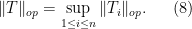
A basic problem in harmonic analysis (as well as in linear algebra, random matrix theory, and high-dimensional geometry) is to estimate the operator norm 


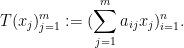
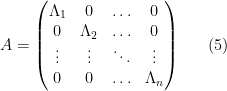
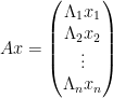
In general, this operator norm is hard to compute precisely, except in special cases. One such special case is that of a diagonal operator, such as that associated to an 


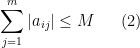
A variant of (1) is Schur’s test, which for simplicity we will phrase in the setting of finite-dimensional operators 
A simple version of this test is as follows: if all the absolute row sums and columns sums of 
 and
and 
 , then
(note that this generalises (the upper bound in) (1).) Indeed, to see (4), it suffices by duality and homogeneity to show that

whenever 


Schur’s test (4) (and its many generalisations to weighted situations, or to Lebesgue or Lorentz spaces) is particularly useful for controlling operators in which the role of oscillation (as reflected in the phase of the coefficients 


To illustrate the basic flavour of the result, let us return to the bound (1), and now consider instead a block-diagonal matrix
where each 


Indeed, the lower bound is trivial (as can be seen by testing 

to decompose an arbitrary vector 

with 
and the upper bound in (6) then follows from a simple computation.
The operator 

When 

The reason for this gain can ultimately be traced back to the “orthogonality” of the


whenever 

The Cotlar-Stein lemma is an extension of this observation to the case where the
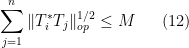
Lemma 1 (Cotlar-Stein lemma) Let
be a finite sequence of bounded linear operators from one Hilbert space
, obeying the bounds
for all
and some
(compare with (2), (3)). Then one has
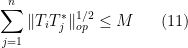


that the hypothesis (11) (or (12)) already gives the bound

on each component
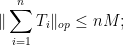
the point of the Cotlar-Stein lemma is that the dependence on 
The Cotlar-Stein lemma was first established by Cotlar in the special case of commuting self-adjoint operators, and then independently by Cotlar and Stein in full generality, with the proof appearing in a subsequent paper of Knapp and Stein.
The Cotlar-Stein lemma is often useful in controlling operators such as singular integral operators or pseudo-differential operators 


Once one is in the almost orthogonal setting, as opposed to the genuinely orthogonal setting, the previous arguments based on orthogonal projection seem to fail completely. Instead, the proof of the Cotlar-Stein lemma proceeds via an elegant application of the tensor power trick (or perhaps more accurately, the power method), in which the operator norm of 

To estimate the right-hand side, we expand out the right-hand side and apply the triangle inequality to bound it by

Recall that when we applied the triangle inequality directly to
To bound (17), we use the basic inequality 


On the other hand, we can group the product by pairs in another way, to obtain the bound of

We bound 


If we then sum this series first in 


for (16). Taking 

Sending 
Remark 1 As observed in a number of places (see e.g. page 318 of Stein’s book, or this paper of Comech, the Cotlar-Stein lemma can be extended to infinite sums
(with the obvious changes to the hypotheses (11), (12)). Indeed, one can show that for any
, the sum
is unconditionally convergent in
Remark 2 If we specialise to the case where all the
Remark 3 One can prove Schur’s test by a similar method. Indeed, starting from the inequality
(which follows easily from the singular value decomposition), we can bound
by
Estimating the other two terms in the summand by
and the claim follows from the tensor power trick as before. On the other hand, in the converse direction, I do not know of any way to prove the Cotlar-Stein lemma that does not basically go through the tensor power argument.


Recall that a (real) topological vector space is a real vector space 


An obvious example of a topological vector space is a finite-dimensional vector space such as 
One way to distinguish the finite and infinite dimensional topological vector spaces is via local compactness. Recall that a topological space is locally compact if every point in that space has a compact neighbourhood. From the Heine-Borel theorem, all finite-dimensional vector spaces (with the usual topology) are locally compact. In infinite dimensions, one can trivially make a vector space locally compact by giving it a trivial topology, but once one restricts to the Hausdorff case, it seems impossible to make a space locally compact. For instance, in an infinite-dimensional normed vector space 

Theorem 1 Every locally compact Hausdorff topological vector space is finite-dimensional.
The first proof of this theorem that I am aware of is by André Weil. There is also a related result:
Theorem 2 Every finite-dimensional Hausdorff topological vector space has the usual topology.
As a corollary, every locally compact Hausdorff topological vector space is in fact isomorphic to
Theorem 2 may seem devoid of content, but it does contain some subtleties, as it hinges crucially on the joint continuity of the vector space operations 

![{\{ (x,y) \in {\bf R}: x+y \not \in [0,1]\}}](https://s0.wp.com/latex.php?latex=%7B%5C%7B+%28x%2Cy%29+%5Cin+%7B%5Cbf+R%7D%3A+x%2By+%5Cnot+%5Cin+%5B0%2C1%5D%5C%7D%7D&bg=ffffff&fg=000000&s=0&c=20201002)
Another near-counterexample comes from the topology of 

As some final examples, consider
Below the fold, I record the textbook proof of Theorem 2 and Theorem 1. There is nothing particularly original in this presentation, but I wanted to record it here for my own future reference, and perhaps these results will also be of interest to some other readers.
If 


where 


for all 


for all 

By combining the Hardy-Littlewood maximal inequality with the Marcinkiewicz interpolation theorem (and the trivial inequality 

for all 


The exact dependence of 


In 1982, Stein gave an elegant argument (with full details appearing in a subsequent paper of Stein and Strömberg), based on the Calderón-Zygmund method of rotations, to eliminate the dependence of
 for each
  depends only on
 The argument is based on an earlier bound of Stein from 1976 on the spherical maximal function
where 
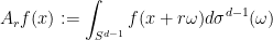
and 


for all (continuous) 
The condition 


The Hardy-Littlewood maximal operator 
for any (continuous) 
At first glance, this observation does not immediately establish Theorem 1 for two reasons. Firstly, Stein’s spherical maximal theorem is restricted to the case when 
We still have to deal with the second objection, namely that constant 

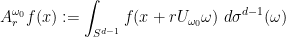
for the

for the 


for any continuous 
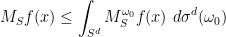
where 


uniformly in 


indeed, one can deduce this from the uniqueness of Haar measure by noting that both the left-hand side and right-hand side are invariant means of 
and thus by Minkowski’s inequality for integrals, we may deduce (5) from (6).
Remark 1 Unfortunately, the method of rotations does not work to show that the constant
for the weak
inequality (1) is independent of dimension, as the weak
quasinorm
is not a genuine norm and does not obey the Minkowski inequality for integrals. Indeed, the question of whether
for some absolute constant
, by comparing the Hardy-Littlewood maximal function with the heat kernel maximal function
The abstract semigroup maximal inequality of Dunford and Schwartz (discussed for instance in these lecture notes of mine) shows that the heat kernel maximal function is of weak-type
, and this can be used, together with a comparison argument, to give the Stein-Strömberg bound. In the converse direction, it is a recent result of Aldaz that if one replaces the balls
.

I recently reposted my favourite logic puzzle, namely the blue-eyed islander puzzle. I am fond of this puzzle because in order to properly understand the correct solution (and to properly understand why the alternative solution is incorrect), one has to think very clearly (but unintuitively) about the nature of knowledge.
There is however an additional subtlety to the puzzle that was pointed out in comments, in that the correct solution to the puzzle has two components, a (necessary) upper bound and a (possible) lower bound (I’ll explain this further below the fold, in order to avoid blatantly spoiling the puzzle here). Only the upper bound is correctly explained in the puzzle (and even then, there are some slight inaccuracies, as will be discussed below). The lower bound, however, is substantially more difficult to establish, in part because the bound is merely possible and not necessary. Ultimately, this is because to demonstrate the upper bound, one merely has to show that a certain statement is logically deducible from an islander’s state of knowledge, which can be done by presenting an appropriate chain of logical deductions. But to demonstrate the lower bound, one needs to show that certain statements are not logically deducible from an islander’s state of knowledge, which is much harder, as one has to rule out all possible chains of deductive reasoning from arriving at this particular conclusion. In fact, to rigorously establish such impossiblity statements, one ends up having to leave the “syntactic” side of logic (deductive reasoning), and move instead to the dual “semantic” side of logic (creation of models). As we shall see, semantics requires substantially more mathematical setup than syntax, and the demonstration of the lower bound will therefore be much lengthier than that of the upper bound.
To complicate things further, the particular logic that is used in the blue-eyed islander puzzle is not the same as the logics that are commonly used in mathematics, namely propositional logic and first-order logic. Because the logical reasoning here depends so crucially on the concept of knowledge, one must work instead with an epistemic logic (or more precisely, an epistemic modal logic) which can properly work with, and model, the knowledge of various agents. To add even more complication, the role of time is also important (an islander may not know a certain fact on one day, but learn it on the next day), so one also needs to incorporate the language of temporal logic in order to fully model the situation. This makes both the syntax and semantics of the logic quite intricate; to see this, one only needs to contemplate the task of programming a computer with enough epistemic and temporal deductive reasoning powers that it would be able to solve the islander puzzle (or even a smaller version thereof, say with just three or four islanders) without being deliberately “fed” the solution. (The fact, therefore, that humans can grasp the correct solution without any formal logical training is therefore quite remarkable.)
As difficult as the syntax of temporal epistemic modal logic is, though, the semantics is more intricate still. For instance, it turns out that in order to completely model the epistemic state of a finite number of agents (such as 1000 islanders), one requires an infinite model, due to the existence of arbitrarily long nested chains of knowledge (e.g. “
Despite all this fearsome complexity, it is still possible to set up both the syntax and semantics of temporal epistemic modal logic in such a way that one can formulate the blue-eyed islander problem rigorously, and in such a way that one has both an upper and a lower bound in the solution. The purpose of this post is to construct such a setup and to explain the lower bound in particular. The same logic is also useful for analysing another well-known paradox, the unexpected hanging paradox, and I will do so at the end of the post. Note though that there is more than one way to set up epistemic logics, and they are not all equivalent to each other.
(On the other hand, for puzzles such as the islander puzzle in which there are only a finite number of atomic propositions and no free variables, one at least can avoid the need to admit predicate logic, in which one has to discuss quantifiers such as 

Our approach here will be a little different from the approach commonly found in the epistemic logic literature, in which one jumps straight to “arbitrary-order epistemic logic” in which arbitrarily long nested chains of knowledge (“


I should warn that this is going to be a rather formal and mathematical post. Readers who simply want to know the answer to the islander puzzle would probably be better off reading the discussion at the puzzle’s own blog post instead.
A topological space 

There are some obvious necessary conditions on the space 

In the converse direction, being Hausdorff and first countable is not always enough to guarantee metrisability, for a variety of reasons. For instance the long line is not metrisable despite being both Hausdorff and first countable, due to a failure of paracompactness, which prevents one from gluing together the local metric structures on this line into a global one. Even after adding in paracompactness, this is still not enough; the real line with the lower limit topology (also known as the Sorgenfrey line) is Hausdorff, first countable, and paracompact, but still not metrisable (because of a failure of second countability despite being separable).
However, there is one important setting in which the Hausdorff and first countability axioms do suffice to give metrisability, and that is the setting of topological groups:
Theorem 1 (Birkhoff-Kakutani theorem) Let
and
are continuous). Then
Remark 1 It is not hard to show that a topological group is Hausdorff if and only if the singleton set
is closed. More generally, in an arbitrary topological group, it is a good exercise to show that the closure of
is then a Hausdorff topological group. Because of this, the study of topological groups can usually be reduced immediately to the study of Hausdorff topological groups. (Indeed, in many texts, topological groups are automatically understood to be an abbreviation for “Hausdorff topological group”.)
The standard proof of the Birkhoff-Kakutani theorem (which we have taken from this book of Montgomery and Zippin) relies on the following Urysohn-type lemma:
Lemma 2 (Urysohn-type lemma) Let
with the following properties:
- (Unique maximum)
, and
for all
.
- (Neighbourhood base) The sets
for
- (Uniform continuity) For every
, there exists an open neighbourhood
for all
and
.
Note that if 
Let us assume Lemma 2 for now and finish the proof of the Birkhoff-Kakutani theorem. We only prove the difficult direction, namely that a Hausdorff first countable topological group 

where 

Clearly 


To put it another way: because 

Now we have to check whether the metric
To verify the former claim, it suffices to show that the map 
Remark 2 The above argument in fact shows that if a group
Now we prove Lemma 2. By first countability, we can find a countable neighbourhood base
of the identity. As

Using the continuity of the group axioms, we can recursively find a sequence of nested open neighbourhoods of the identity

such that each 


For every dyadic rational 


where 

for all 

We now set

with the understanding that 
Remark 3 A very similar argument to the one above also establishes that every topological group
Notice that the function 


- (Continuity)
and
are continuous on their domains of definition.
- (Identity) For any
,
and
are well-defined and equal to
.
- (Inverse) For any
,
and
are well-defined and equal to
is well-defined and equal to
- (Local associativity) If
are such that
,
,
, and
are all well-defined, then
.
Informally, one can view a local group as a topological group in which the closure axiom has been almost completely dropped, but with all the other axioms retained. A basic way to generate a local group is to start with an ordinary topological group 

Remark 4 Another important example of a local group is that of a group chunk, in which the sets
Zariski-open, and the group operations birational on their domains of definition. This is somewhat analogous to the notion of a “
group” in additive combinatorics. There are a number of group chunk theorems, starting with a theorem of Weil in the algebraic setting, which roughly speaking assert that a generic portion of a group chunk can be identified with the generic portion of a genuine group.
We then have
Theorem 3 (Birkhoff-Kakutani theorem for local groups) Let
of the identity which is metrisable.
Proof: (Sketch) It is not difficult to see that in a local group 


My motivation for studying local groups is that it turns out that there is a correspondence (first observed by Hrushovski) between the concept of an approximate group in additive combinatorics, and a locally compact local group in topological group theory; I hope to discuss this correspondence further in a subsequent post.
Suppose one has a measure space 


One standard way to proceed here is to study the maximal operator

and aim to establish a weak-type maximal inequality

for all 


A standard approximation argument using (1) then shows that 
In the case of norm convergence (in which one asks for

for some 
Returning to pointwise almost everywhere convergence, the answer in general is “yes”. Consider for instance the rank one operators
![\displaystyle T_n f(x) := 1_{[n,n+1]} \int_0^1 f(y)\ dy](https://s0.wp.com/latex.php?latex=%5Cdisplaystyle+T_n+f%28x%29+%3A%3D+1_%7B%5Bn%2Cn%2B1%5D%7D+%5Cint_0%5E1+f%28y%29%5C+dy&bg=ffffff&fg=000000&s=0&c=20201002)
from 


In spite of this, a remarkable observation of Stein, now known as Stein’s maximal principle, asserts that the maximal inequality is necessary to prove pointwise almost everywhere convergence, if one is working on a compact group and the operators
Theorem 1 (Stein maximal principle) Let
, let
, and let
This is not quite the most general vesion of the principle; some additional variants and generalisations are given in the original paper of Stein. For instance, one can replace the discrete sequence 


And unsurprisingly, most of the proofs of this (difficult) theorem have proceeded by first establishing (3), and Stein’s maximal principle strongly suggests that this is the optimal way to try to prove this theorem.
On the other hand, the theorem does fail for 


Stein’s principle is restricted to compact groups (such as the torus 


![{T_n f := f * 1_{[n,n+1]}}](https://s0.wp.com/latex.php?latex=%7BT_n+f+%3A%3D+f+%2A+1_%7B%5Bn%2Cn%2B1%5D%7D%7D&bg=ffffff&fg=000000&s=0&c=20201002)

Stein’s argument from his 1961 paper can be viewed nowadays as an application of the probabilistic method; starting with a sequence of increasingly bad counterexamples to the maximal inequality (1), one randomly combines them together to create a single “infinitely bad” counterexample. To make this idea work, Stein employs two basic ideas:
- The random rotations (or random translations) trick. Given a subset
translates
of
- The random sums trick Given a collection
of signed functions that may possibly cancel each other in a deterministic sum
, one can perform a random sum
instead to obtain a random function whose magnitude will usually be comparable to the square function
; this can be made rigorous by concentration of measure results, such as Khintchine’s inequality.
These ideas have since been used repeatedly in harmonic analysis. For instance, I used the random rotations trick in a recent paper with Jordan Ellenberg and Richard Oberlin on Kakeya-type estimates in finite fields. The random sums trick is by now a standard tool to build various counterexamples to estimates (or to convergence results) in harmonic analysis, for instance being used by Fefferman in his famous paper disproving the boundedness of the ball multiplier on 

Another use of the random rotations trick, closely related to Theorem 1, is the Nikishin-Stein factorisation theorem. Here is Stein’s formulation of this theorem:
Theorem 2 (Stein factorisation theorem) Let
, and let
be a bounded linear operator commuting with translations and obeying the estimate
for all
. Then
, with
for all
depending only on
.


This result is trivial with 


Stein’s factorisation theorem (or more precisely, a variant of it) is useful in the theory of Kakeya and restriction theorems in Euclidean space, as first observed by Bourgain.
In 1970, Nikishin obtained the following generalisation of Stein’s factorisation theorem in which the translation-invariance hypothesis can be dropped, at the cost of excluding a set of small measure:
Theorem 3 (Nikishin-Stein factorisation theorem) Let
for all
, there exists a subset
such that

 depending only on
  .
.One can recover Theorem 2 from Theorem 3 by an averaging argument to eliminate the exceptional set; we omit the details.
Recall that a (complex) abstract Lie algebra is a complex vector space ![{[]: {\mathfrak g} \times {\mathfrak g} \rightarrow {\mathfrak g}}](https://s0.wp.com/latex.php?latex=%7B%5B%5D%3A+%7B%5Cmathfrak+g%7D+%5Ctimes+%7B%5Cmathfrak+g%7D+%5Crightarrow+%7B%5Cmathfrak+g%7D%7D&bg=ffffff&fg=000000&s=0&c=20201002)
![\displaystyle [[X,Y],Z] + [[Y,Z],X] + [[Z,X],Y] = 0. \ \ \ \ \ (1)](https://s0.wp.com/latex.php?latex=%5Cdisplaystyle++%5B%5BX%2CY%5D%2CZ%5D+%2B+%5B%5BY%2CZ%5D%2CX%5D+%2B+%5B%5BZ%2CX%5D%2CY%5D+%3D+0.+%5C+%5C+%5C+%5C+%5C+%281%29&bg=ffffff&fg=000000&s=0&c=20201002)
(One can of course define Lie algebras over other fields than the complex numbers 
An important special case of the abstract Lie algebras are the concrete Lie algebras, in which 

![\displaystyle [X,Y] := XY-YX.](https://s0.wp.com/latex.php?latex=%5Cdisplaystyle++%5BX%2CY%5D+%3A%3D+XY-YX.&bg=ffffff&fg=000000&s=0&c=20201002)
It is easy to verify that every concrete Lie algebra is an abstract Lie algebra. In the converse direction, we have
Theorem 1 Every abstract Lie algebra is isomorphic to a concrete Lie algebra.
To prove this theorem, we introduce the useful algebraic tool of the universal enveloping algebra 
![\displaystyle [X,Y] = XY - YX. \ \ \ \ \ (2)](https://s0.wp.com/latex.php?latex=%5Cdisplaystyle++%5BX%2CY%5D+%3D+XY+-+YX.+%5C+%5C+%5C+%5C+%5C+%282%29&bg=ffffff&fg=000000&s=0&c=20201002)
This algebra is described by the Poincaré-Birkhoff-Witt theorem, which asserts that given an ordered basis 

where 


![{XY = YX + [X,Y]}](https://s0.wp.com/latex.php?latex=%7BXY+%3D+YX+%2B+%5BX%2CY%5D%7D&bg=ffffff&fg=000000&s=0&c=20201002)
The abstract Lie algebra 


In the converse direction, every representation 

One drawback of Theorem 1 is that the space
Theorem 2 (Ado’s theorem) Every finite-dimensional abstract Lie algebra is isomorphic to a concrete Lie algebra over a finite-dimensional vector space
Among other things, this theorem can be used (in conjunction with the Baker-Campbell-Hausdorff formula) to show that every abstract (finite-dimensional) Lie group (or abstract local Lie group) is locally isomorphic to a linear group. (It is well-known, though, that abstract Lie groups are not necessarily globally isomorphic to a linear group, but we will not discuss these global obstructions here.)
Ado’s theorem is surprisingly tricky to prove in general, but some special cases are easy. For instance, one can try using the adjoint representation 
![{X: Y \mapsto [X,Y]}](https://s0.wp.com/latex.php?latex=%7BX%3A+Y+%5Cmapsto+%5BX%2CY%5D%7D&bg=ffffff&fg=000000&s=0&c=20201002)
![{Z({\mathfrak g}) := \{ X \in {\mathfrak g}: [X,Y]=0 \hbox{ for all } Y \in {\mathfrak g}\}}](https://s0.wp.com/latex.php?latex=%7BZ%28%7B%5Cmathfrak+g%7D%29+%3A%3D+%5C%7B+X+%5Cin+%7B%5Cmathfrak+g%7D%3A+%5BX%2CY%5D%3D0+%5Chbox%7B+for+all+%7D+Y+%5Cin+%7B%5Cmathfrak+g%7D%5C%7D%7D&bg=ffffff&fg=000000&s=0&c=20201002)
The adjoint representation does not suffice, by itself, to prove Ado’s theorem in the non-semisimple case. However, it does provide an important reduction in the proof, namely it reduces matters to showing that every finite-dimensional Lie algebra 
It remains to find a finite-dimensional representation of 

This construction gives a faithful finite-dimensional representation of the centre
This procedure is a little tricky to execute in general, but becomes simpler in the nilpotent case, in which the lower central series ![{{\mathfrak g}_1 := {\mathfrak g}; {\mathfrak g}_{n+1} := [{\mathfrak g}, {\mathfrak g}_n]}](https://s0.wp.com/latex.php?latex=%7B%7B%5Cmathfrak+g%7D_1+%3A%3D+%7B%5Cmathfrak+g%7D%3B+%7B%5Cmathfrak+g%7D_%7Bn%2B1%7D+%3A%3D+%5B%7B%5Cmathfrak+g%7D%2C+%7B%5Cmathfrak+g%7D_n%5D%7D&bg=ffffff&fg=000000&s=0&c=20201002)
Theorem 3 (Ado’s theorem for nilpotent Lie algebras) Let
be a finite-dimensional nilpotent Lie algebra. Then there exists a finite-dimensional faithful representation
of
, i.e. one has
for all
.
The second conclusion of Ado’s theorem here is useful for induction purposes. (By Engel’s theorem, this conclusion is also equivalent to the assertion that every element of 
Below the fold, I give a proof of Theorem 3, and then extend the argument to cover the full strength of Ado’s theorem. This is not a new argument – indeed, I am basing this particular presentation from the one in Fulton and Harris – but it was an instructive exercise for me to try to extract the proof of Ado’s theorem from the more general structural theory of Lie algebras (e.g. Engel’s theorem, Lie’s theorem, Levi decomposition, etc.) in which the result is usually placed. (However, the proof I know of still needs Engel’s theorem to establish the solvable case, and the Levi decomposition to then establish the general case.)
Igor Rodnianski and I have just uploaded to the arXiv our paper “Effective limiting absorption principles, and applications“, submitted to Communications in Mathematical Physics. In this paper we derive limiting absorption principles (of type discussed in this recent post) for a general class of Schrödinger operators 


To begin with, we make no hypotheses about the topology or geodesic geometry of the manifold
It is well known that such Schrödinger operators 


for 


It turns out to be convenient to distinguish between three regimes:
- The high-energy regime
;
- The medium-energy regime
; and
- The low-energy regime
.
Our methods actually apply more or less uniformly to all three regimes, but the nature of the conclusions is quite different in each of the three regimes.
The high-energy regime

where 

The exponent 
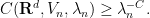
In the medium and low energy regimes one needs to work harder. In the medium energy regime

for all asymptotically conic manifolds (trapping or not) and all short-range potentials. To establish this bound, we have to supplement the existing tools of the positive commutator method and Carleman inequalities with an additional ODE-type analysis of various energies of the solution 
The methods also extend to the low-energy regime 

that blew up at a large polynomial rate at the origin. Furthermore, by carefully designing a sequence of potentials 

This shows that if one wants bounds that are uniform in the potential
Interestingly, though, if we fix the potential

in the low-energy regime (but note carefully here that the constant 


As applications of our limiting absorption estimates, we give local smoothing and dispersive estimates for solutions (as well as the closely related RAGE type theorems) to the time-dependent Schrödinger and wave equations, and also reprove standard facts about the spectrum of Schrödinger operators in this setting.

Recent Comments