Tate’s proof of the functional equation

The Riemann zeta function , defined for by the formula

(1)

where are the natural numbers, and extended meromorphically to other values of s by analytic continuation, obeys the remarkable functional equation

(2)

where

(3)

is the Riemann Xi function,

(4)

is the Gamma factor at infinity, and the Gamma function is defined for by

(5)

and extended meromorphically to other values of s by analytic continuation.

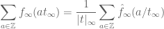
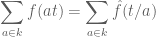
There are many proofs known of the functional equation (2).  One of them (dating back to Riemann himself) relies on the Poisson summation formula

(6)

for the reals and , where is a Schwartz function, is the usual Archimedean absolute value on , and

(7)

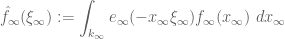
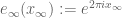
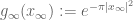
is the Fourier transform on , with being the standard character on .  (The reason for this rather strange notation for the real line and its associated structures will be made clearer shortly.)  Applying this formula to the (Archimedean) Gaussian function

, (8)

which is its own (additive) Fourier transform, and then applying the multiplicative Fourier transform (i.e. the Mellin transform), one soon obtains (2).  (Riemann also had another proof of the functional equation relying primarily on contour integration, which I will not discuss here.)  One can “clean up” this proof a bit by replacing the Gaussian by a Dirac delta function, although one now has to work formally and “renormalise” by throwing away some infinite terms.  (One can use the theory of distributions to make this latter approach rigorous, but I will not discuss this here.)  Note how this proof combines the additive Fourier transform with the multiplicative Fourier transform.  [Continuing with this theme, the Gamma function (5) is an inner product between an additive character and a multiplicative character , and the zeta function (1) can be viewed both additively, as a sum over n, or multiplicatively, as an Euler product.]

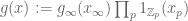
In the famous thesis of Tate, the above argument was reinterpreted using the language of the adele ring , with the Poisson summation formula (4) on replaced by the Poisson summation formula

(9)

on , where is the rationals, , and f is now a Schwartz-Bruhat function on .  Applying this formula to the adelic (or global) Gaussian function , which is its own Fourier transform, and then using the adelic Mellin transform, one again obtains (2).  Again, the proof can be cleaned up by replacing the Gaussian with a Dirac mass, at the cost of making the computations formal (or requiring the theory of distributions).

In this post I will write down both Riemann’s proof and Tate’s proof together (but omitting some technical details), to emphasise the fact that they are, in some sense, the same proof.  However, Tate’s proof gives a high-level clarity to the situation (in particular, explaining more adequately why the Gamma factor at infinity (4) fits seamlessly with the Riemann zeta function (1) to form the Xi function (2)), and allows one to generalise the functional equation relatively painlessly to other zeta-functions and L-functions, such as Dedekind zeta functions and Hecke L-functions.

[Note: the material here is very standard in modern algebraic number theory; the post here is partially for my own benefit, as most treatments of this topic in the literature tend to operate in far higher levels of generality than I would prefer.]

Global existence and uniqueness results for weak solutions of the focusing mass-critical non-linear Schrödinger equation

I’ve just uploaded to the arXiv the paper “Global existence and uniqueness results for weak solutions of the focusing mass-critical non-linear Schrödinger equation“, submitted to Analysis & PDE.  This paper is concerned with solutions to the focusing mass-critical NLS equation

, (1)

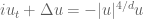
where the only regularity we assume on the solution is that the mass is finite and locally bounded in time.  (For sufficiently strong notions of solution, the mass is in fact conserved, but part of the point with this paper is that mass conservation breaks down when the solution becomes too weak.)  Note that the mass is dimensionless (i.e. scale-invariant) with respect to the natural scale invariance for this equation.  For various technical reasons I work in high dimensions (this in particular allows the nonlinearity in (1) to be locally integrable in space).

In the classical (smooth) category, there is no ambiguity as to what it means for a function u to “solve” an equation such as (1); but once one is in a low regularity class (such as the class of finite mass solutions), there are several competing notions of solution, in particular the notions of a strong solution and a weak solution.  To oversimplify a bit, both strong and weak solutions solve (1) in a distributional sense, but strong solutions are also continuous in time (in the space of functions of finite mass).   A canonical example here is given by the pseudoconformally transformed soliton blowup solution

(2)

to (1), where Q is a solution to the ground state equation 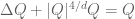.  This solution is a strong solution on (say) the time interval , but cannot be continued as a strong solution beyond time zero due to the discontinuity at t=0.  Nevertheless, it can be continued as a weak solution by extending by zero at t=0 and at (or alternatively, one could extend for using (2); thus there is no uniqueness for the initial value problem in the weak solution class. Note this example also shows that weak solutions need not conserve mass; all the mass in (1) concentrates into the spatial origin as and disappears in the limit t=0).

There is a slightly stronger notion than a strong solution, which I call a Strichartz-class solution, in which one adds an additional regularity assumption .  This assumption is natural from the point of view of Strichartz estimates, which are a major tool in the analysis of such equations.

There is a vast theory for the initial value problem for these sorts of equations, but basically one has the following situation: in the category of Strichartz class solutions, one has local existence and uniqueness, but not global existence (as the example (2) already shows); at the other extreme, in the category of weak solutions, one has global existence, but not uniqueness (as (2) again shows).

(This contrast between strong and weak solutions shows up in many other PDE as well.  For instance, global existence of smooth solutions to the Navier-Stokes equation is one of the Clay Millennium problems that I have blogged about before, but global existence of weak solutions is quite easy with today’s technology and was first done by Leray back in 1933.)

In this paper, I introduce a new solution class, which I call the semi-Strichartz class; rather than being continuous in time, it varies right-continuously (in both the mass space and the Strichartz space) in time in the future of the initial time , and left-continuously in the past of .  With this tweak of the definition, it turns out that one has both global existence and uniqueness in this class.  (For instance, if one started with the initial data u(-1) given by (2) at time t=-1, the unique global semi-Strichartz solution from this initial data would be given by (2) for negative times and by zero for non-negative times.)  This notion of solution is analogous (but much, much simpler than) the notion of Ricci flow with surgery used by Hamilton and Perelman; basically, every time a singularity develops, the semi-Strichartz solution removes the portion of mass that was becoming discontinuous, leaving only the non-singular portion of the solution to continue onwards in time.

(Timothy Chow) Out-of-print math books

[This post is authored by Timothy Chow.]

I recently had a frustrating experience with a certain out-of-print mathematics text that I was interested in.  A couple of used copies were listed at over $150 a pop on Bookfinder.com, but that was more than I was willing to pay.  I wrote to the American Mathematical Society asking if they were interested in bringing the book back into print.  To their credit, they took my request seriously, and solicited the opinions of some other mathematicians.

Unfortunately, these referees all said that the field in question was not active, and in any case there was a more recent text that was a better reference.  So the AMS rejected my proposal.  I have to say that I was surprised, because the referees did not back up their opinions with any facts, and I knew that in addition to the high price that the book commanded on the used-book market, there was some circumstantial evidence that it was in demand.  A MathSciNet search confirmed my belief that, contrary to what the referees had said, the field was most definitely active.  Plus, another text on the same subject that Dover had recently brought back into print had a fine Amazon sales rank (much higher than that of the recent text cited by the referees).

A colleague then suggested that maybe I should instead contact the author directly, asking him to regain the copyright from the publisher.  The author could then make the book available on his website or pursue print-on-demand options, if conventional publishers were not interested. I tried this, but was again surprised to discover that the author thought it was not worth the trouble to get the copyright back, let alone to make the text available.  Again the argument was that, allegedly, nobody was interested in the book.

In both cases I was frustrated because I did not know how to find other people who were interested in the same book, to prove to the AMS or the author that there were in fact many of us who wanted to see the book back in print.

Now for the good news.  After hearing my story, Klaus Schmid promptly set up a prototype website at

http://outofprintmath.blogspot.com

Anyone can go to this site and suggest a book, or vote for books that others have suggested.  This is precisely the kind of information that I believe would have greatly helped me argue my case.  Of course, the site works only if people know about it, so if you like the idea, please spread the word to your friends and colleagues.

It might be that a better long-term solution than Schmid’s site is to convince a bookselling website to tally votes of this sort, because such a site will catch users “red-handed” searching for an out-of-print book.  I have tried to contact some sites with this suggestion; so far, Booksprice.com and Fetchbook.info have said that they like the idea and may eventually implement it.  In the meantime, hopefully Schmid’s site will  become a useful tool in its own right.

Let me conclude with a question.  What else can we be doing to increase the availability of out-of-print books, especially those that are still copyrighted?  Several people have told me that the solution is for authors to regain the copyrights to their out-of-print books and make their books available themselves, but authors are often too busy (if they are not deceased!).  What can we do to help in such situations?

Classification of Almost Quarter-Pinched Manifolds

Peter Petersen and I have just uploaded to the arXiv our paper, “Classification of Almost Quarter-Pinched Manifolds“, submitted to Proc. Amer. Math. Soc..  This is perhaps the shortest paper (3 pages) I have ever been involved in, because we were fortunate enough that we could simply cite (as a black box) a reference for every single fact that we needed here.

The paper is related to the famous sphere theorem from Riemannian geometry.  This theorem asserts that any n-dimensional complete simply connected Riemannian manifold which was strictly quarter-pinched (i.e. the sectional curvatures all in the interval for some ) must necessarily be homeomorphic to the n-sphere .    (In dimensions 3 or less, this already follows from simple connectedness thanks to the Poincaré conjecture (and Myers theorem), so the theorem is really only interesting in higher dimensions.  One can easily drop the simple connectedness hypothesis by passing to a universal cover, but then one has to admit sphere quotients as well as spheres.)

Due to the existence of exotic spheres in higher dimensions, being homeomorphic to a sphere does not necessarily imply being diffeomorphic to a sphere.  (For instance, an example of an exotic sphere with positive sectional curvature (but not quarter-pinched) was recently constructed by Petersen and Wilhelm.)  Nevertheless, Brendle and Schoen recently proved the diffeomorphic version of the sphere theorem: every strictly quarter-pinched complete simply connected Riemannian manifold is diffeomorphic to a sphere.  The proof is based on Ricci flow, and involves three main steps:

1. A verification that if M is quarter-pinched, then the manifold has non-negative isotropic curvature.  (The same statement is true without adding the two additional flat dimensions, but these additional dimensions are very convenient for simplifying the analysis by allowing certain two-planes to wander freely in the product tangent space.)
2. A verification that the property of having non-negative isotropic curvature is preserved by Ricci flow.  (By contrast, the quarter-pinched property is not preserved by Ricci flow.)
3. The pinching theory of Böhm and Wilking, which is a refinement of the work of Hamilton (who handled the three and four-dimensional cases).

Brendle and Schoen in fact proved a slightly stronger statement in which the curvature bound K is allowed to vary with position x, but we will not discuss this strengthening here.

The quarter-pinching is sharp; the Fubini-Study metric on complex projective spaces is non-strictly quarter-pinched (the sectional curvatures lie in but is not homeomorphic to a sphere).  Nevertheless, by refining the above methods, an endpoint result was established by Brendle and Schoen (see also a later refinement by Seshadri): any complete simply-connected manifold which is non-strictly quarter-pinched is diffeomorphic to either a sphere or a compact rank one symmetric space (or CROSS, for short) such as complex projective space.  (In the latter case one also has some further control on the metric, which we will not detail here.)  The homeomorphic version of this statement was established earlier by Berger and by Klingenberg.

Our result pushes this further by an epsilon.  More precisely, we show for each dimension n that there exists such that any -pinched complete simply connected manifold (i.e. the curvatures lie in ) is diffeomorphic to either a sphere or a CROSS.  (The homeomorphic version of this statement was established earlier in even dimensions by Berger.)  We do not know if can be made independent of n.

The Mobius function is strongly orthogonal to nilsequences

Ben Green and I have just uploaded to the arXiv our paper, “The Möbius function is asymptotically orthogonal to nilsequences“, which is a sequel to our earlier paper “The quantitative behaviour of polynomial orbits on nilmanifolds“, which I talked about in this post.  In this paper, we apply our previous results on quantitative equidistribution polynomial orbits in nilmanifolds to settle the Möbius and nilsequences conjecture from our earlier paper, as part of our program to detect and count solutions to linear equations in primes.  (The other major plank of that program, namely the inverse conjecture for the Gowers norm, remains partially unresolved at present.)  Roughly speaking, this conjecture asserts the asymptotic orthogonality

(1)

between the Möbius function and any Lipschitz nilsequence f(n), by which we mean a sequence of the form for some orbit in a nilmanifold , and some Lipschitz function on that nilmanifold.  (The implied constant can depend on the nilmanifold and on the Lipschitz constant of F, but it is important that it be independent of the generator g of the orbit or the base point x.)  The case when f is constant is essentially the prime number theorem; the case when f is periodic is essentially the prime number theorem in arithmetic progressions.  The case when f is almost periodic (e.g. for some irrational ) was established by Davenport, using the method of Vinogradov.  The case when f was a 2-step nilsequence (such as the quadratic phase ; bracket quadratic phases such as can also be covered by an approximation argument, though the logarithmic decay in (1) is weakened as a consequence) was done by Ben and myself a few years ago, by a rather ad hoc adaptation of Vinogradov’s method.  By using the equidistribution theory of nilmanifolds, we were able to apply Vinogradov’s method more systematically, and in fact the proof is relatively short (20 pages), although it relies on the 64-page predecessor paper on equidistribution.  I’ll talk a little bit more about the proof after the fold.

There is an amusing way to interpret the conjecture (using the close relationship between nilsequences and bracket polynomials) as an assertion of the pseudorandomness of the Liouville function from a computational complexity perspective.    Suppose you possess a calculator with the wonderful property of being infinite precision: it can accept arbitrarily large real numbers as input, manipulate them precisely, and also store them in memory.  However, this calculator has two limitations.  Firstly, the only operations available are addition, subtraction, multiplication, integer part , fractional part , memory store (into one of O(1) registers), and memory recall (from one of these O(1) registers).  In particular, there is no ability to perform division.  Secondly, the calculator only has a finite display screen, and when it shows a real number, it only shows O(1) digits before and after the decimal point.  (Thus, for instance, the real number 1234.56789 might be displayed only as .)

Now suppose you play the following game with an opponent.

1. The opponent specifies a large integer d.
2. You get to enter in O(1) real constants of your choice into your calculator.  These can be absolute constants such as and , or they can depend on d (e.g. you can enter in ).
3. The opponent randomly selects an d-digit integer n, and enters n into one of the registers of your calculator.
4. You are allowed to perform O(1) operations on your calculator and record what is displayed on the calculator’s viewscreen.
5. After this, you have to guess whether the opponent’s number n had an odd or even number of prime factors (i.e. you guess .)
6. If you guess correctly, you win $1; otherwise, you lose $1.

For instance, using your calculator you can work out the first few digits of , provided of course that you entered the constants and in advance.  You can also work out the leading digits of n by storing in advance, and computing the first few digits of .

Our theorem is equivalent to the assertion that as d goes to infinity (keeping the O(1) constants fixed), your probability of winning this game converges to 1/2; in other words, your calculator becomes asymptotically useless to you for the purposes of guessing whether n has an odd or even number of prime factors, and you may as well just guess randomly.

[I should mention a recent result in a similar spirit by Mauduit and Rivat; in this language, their result asserts that knowing the last few digits of the digit-sum of n does not increase your odds of guessing correctly.]

Hassell’s proof of scarring for the Bunimovich stadium

Last year, as part of my “open problem of the week” series (now long since on hiatus), I featured one of my favorite problems, namely that of establishing scarring for the Bunimovich stadium.  I’m now happy to say that this problem has been solved (for generic stadiums, at least, and for phase space scarring rather than physical space scarring) by my old friend (and fellow Aussie), Andrew Hassell, in a recent preprint.  Congrats Andrew!

Actually, the argument is beautifully simple and short (the paper is a mere 9 pages), though it of course uses the basic theory of eigenfunctions on domains, such as Weyl’s law, and I can give the gist of it here (suppressing all technical details).

The Black-Scholes equation

Some time ago, I wrote a short unpublished note (mostly for my own benefit) when I was trying to understand the derivation of the Black-Scholes equation in financial mathematics, which computes the price of various options under some assumptions on the underlying financial model.  In order to avoid issues relating to stochastic calculus, Itō’s formula, etc. I only considered a discrete model rather than a continuous one, which makes the mathematics much more elementary.  I was recently asked about this note, and decided that it would be worthwhile to expand it into a blog article here.  The emphasis here will be on the simplest models rather than the most realistic models, in order to emphasise the beautifully simple basic idea behind the derivation of this formula.

The basic type of problem that the Black-Scholes equation solves (in particular models) is the following.  One has an underlying financial instrument S, which represents some asset which can be bought and sold at various times t, with the per-unit price of the instrument varying with t.  (For the mathematical model, it is not relevant what type of asset S actually is, but one could imagine for instance that S is a stock, a commodity, a currency, or a bond.)  Given such an underlying instrument S, one can create options based on S and on some future time , which give the buyer and seller of the options certain rights and obligations regarding S at an expiration time .  For instance,

1. A call option for S at time and at a strike price P gives the buyer of the option the right (but not the obligation) to buy a unit of S from the seller of the option at price P at time (conversely, the seller of the option has the obligation but not the right to sell a unit of S to the buyer of the option at time , if the buyer so requests).
2. A put option for S at time and at a strike price P gives the buyer of the option the right (but not the obligation) to sell a unit of S to the seller of the option at price P at time (and conversely, the seller of the option has the obligation but not the right to buy a unit of S from the buyer of the option at time , if the buyer so requests).
3. More complicated options, such as straddles and collars, can be formed by taking linear combinations of call and put options, e.g. simultaneously buying or selling a call and a put option.  One can also consider “American options” which offer rights and obligations for an interval of time, rather than the “European options” described above which only apply at a fixed time .  The Black-Scholes formula applies only to European options, though extensions of this theory have been applied to American options.

The problem is this: what is the “correct” price, at time , to assign to an European option (such as a put or call option) at a future expiration time ?  Of course, due to the volatility of the underlying instrument S, the future price of this instrument is not known at time .  Nevertheless – and this is really quite a remarkable fact – it is still possible to compute deterministically, at time , the price of an option that depends on that unknown price , under certain assumptions (one of which is that one knows exactly how volatile the underlying instrument is).