
You are currently browsing the category archive for the ‘math.SP’ category.
Marcel Filoche, Svitlana Mayboroda, and I have just uploaded to the arXiv our preprint “The effective potential of an 


Suppose one has an eigenfunction

 , where
  is the Laplacian on
  ,
,  is a potential, and
  is an energy. Where would one expect the eigenfunction
  to be concentrated? If the potential
  is smooth and slowly varying, the correspondence principle suggests that the eigenfunction should be mostly concentrated in the potential energy wells
  , with an exponentially decaying amount of tunnelling between the wells. One way to rigorously establish such an exponential decay is through an argument of Agmon, which we will sketch later in this post, which gives an exponentially decaying upper bound (in an
  sense) of eigenfunctions in terms of the distance to the wells
  in terms of a certain “Agmon metric” on determined by the potential and energy level (or any upper bound
  on this energy). Similar exponential decay results can also be obtained for discrete Schrödinger matrix models, in which the domain is replaced with a discrete set such as the lattice
  , and the Laplacian is replaced by a discrete analogue such as a graph Laplacian.
When the potential 


There are now several explanations for why this particular choice 


These particular explanations seem rather specific to the Schrödinger equation (continuous or discrete); we have for instance not been able to find similar identities to explain an effective potential for the bi-Schrödinger operator 
In this paper, we demonstrate the (perhaps surprising) fact that effective potentials continue to exist for operators that bear very little resemblance to Schrödinger operators. Our chosen model is that of an 


 is normalised in
  , where the connectivity
  is the maximum number of non-zero entries of in any row or column,
  are the coefficients of , and
  is a certain moderately complicated but explicit metric function on the spatial domain. Informally, this inequality asserts that the eigenfunction
  should decay like
  or faster. Indeed, our numerics show a very strong log-linear relationship between and
  , although it appears that our exponent
  is not quite optimal. We also provide an associated localisation result which is technical to state but very roughly asserts that a given eigenvector will in fact be localised to a single connected component of
  unless there is a resonance between two wells (by which we mean that an eigenvalue for a localisation of associated to one well is extremely close to an eigenvalue for a localisation of associated to another well); such localisation is also strongly supported by numerics. (Analogous results for Schrödinger operators had been previously obtained by the previously mentioned paper of Arnold, David, Jerison, and my two coauthors, and to quantum graphs in a very recent paper of Harrell and Maltsev.)
Our approach is based on Agmon’s methods, which we interpret as a double commutator method, and in particular relying on exploiting the negative definiteness of certain double commutator operators. In the case of Schrödinger operators 

![\displaystyle \langle [[-\Delta+V,g],g] u, u \rangle = -2\int_{{\bf R}^d} |\nabla g|^2 |u|^2\ dx \leq 0 \ \ \ \ \ (2)](https://s0.wp.com/latex.php?latex=%5Cdisplaystyle++%5Clangle+%5B%5B-%5CDelta%2BV%2Cg%5D%2Cg%5D+u%2C+u+%5Crangle+%3D+-2%5Cint_%7B%7B%5Cbf+R%7D%5Ed%7D+%7C%5Cnabla+g%7C%5E2+%7Cu%7C%5E2%5C+dx+%5Cleq+0+%5C+%5C+%5C+%5C+%5C+%282%29&bg=ffffff&fg=000000&s=0&c=20201002)
![\displaystyle \langle g [\psi, -\Delta+V] u, g \psi u \rangle = \frac{1}{2} \langle [[-\Delta+V, g \psi],g\psi] u, u \rangle](https://s0.wp.com/latex.php?latex=%5Cdisplaystyle++%5Clangle+g+%5B%5Cpsi%2C+-%5CDelta%2BV%5D+u%2C+g+%5Cpsi+u+%5Crangle+%3D+%5Cfrac%7B1%7D%7B2%7D+%5Clangle+%5B%5B-%5CDelta%2BV%2C+g+%5Cpsi%5D%2Cg%5Cpsi%5D+u%2C+u+%5Crangle+&bg=ffffff&fg=000000&s=0&c=20201002)
![\displaystyle -\frac{1}{2} \langle [[-\Delta+V, g],g] \psi u, \psi u \rangle](https://s0.wp.com/latex.php?latex=%5Cdisplaystyle+-%5Cfrac%7B1%7D%7B2%7D+%5Clangle+%5B%5B-%5CDelta%2BV%2C+g%5D%2Cg%5D+%5Cpsi+u%2C+%5Cpsi+u+%5Crangle+&bg=ffffff&fg=000000&s=0&c=20201002)
 after a brief calculation. The double commutator identity then tells us that
 ![\displaystyle \langle g [\psi, -\Delta+V] u, g \psi u \rangle \leq \int_{{\bf R}^d} |\nabla g|^2 |\psi u|^2\ dx.](https://s0.wp.com/latex.php?latex=%5Cdisplaystyle++%5Clangle+g+%5B%5Cpsi%2C+-%5CDelta%2BV%5D+u%2C+g+%5Cpsi+u+%5Crangle+%5Cleq+%5Cint_%7B%7B%5Cbf+R%7D%5Ed%7D+%7C%5Cnabla+g%7C%5E2+%7C%5Cpsi+u%7C%5E2%5C+dx.&bg=ffffff&fg=000000&s=0&c=20201002) to be a non-negative weight and let
to be a non-negative weight and let  for an eigenfunction , then we can write
 ![\displaystyle [\psi, -\Delta+V] u = [\psi, -\Delta+V - E] u = \psi (-\Delta+V - E) u](https://s0.wp.com/latex.php?latex=%5Cdisplaystyle++%5B%5Cpsi%2C+-%5CDelta%2BV%5D+u+%3D+%5B%5Cpsi%2C+-%5CDelta%2BV+-+E%5D+u+%3D+%5Cpsi+%28-%5CDelta%2BV+-+E%29+u&bg=ffffff&fg=000000&s=0&c=20201002)

 . If we select
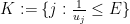
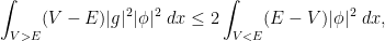
  , we obtain the clean inequality
  to be a function which equals on the wells but increases exponentially away from these wells, in such a way that
 away from the wells. This is basically the classic exponential decay estimate of Agmon; one can basically take to be the distance to the wells with respect to the Euclidean metric conformally weighted by a suitably normalised version of
  . If we instead select to be the landscape function
 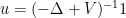 , (3) then gives
  appropriately this gives an exponential decay estimate away from the effective wells
  , using a metric weighted by
  .
.
It turns out that this argument extends without much difficulty to the
![\displaystyle \langle [[A,D],D] u, u \rangle = \sum_{i \neq j} a_{ij} u_i u_j (d_{ii} - d_{jj})^2 \leq 0](https://s0.wp.com/latex.php?latex=%5Cdisplaystyle++%5Clangle+%5B%5BA%2CD%5D%2CD%5D+u%2C+u+%5Crangle%09%3D+%5Csum_%7Bi+%5Cneq+j%7D+a_%7Bij%7D+u_i+u_j+%28d_%7Bii%7D+-+d_%7Bjj%7D%29%5E2+%5Cleq+0&bg=ffffff&fg=000000&s=0&c=20201002)
 . The remainder of the Agmon type arguments go through after making the natural modifications.
Numerically we have also found some aspects of the landscape theory to persist beyond the
Suppose we have an 

where 


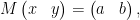
where 


Using the invertibility of

and substituting this into the second equation yields

and thus (assuming that 

and then inserting this back into (1) gives

Comparing this with
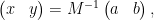
we have managed to express the inverse of


One can consider the inverse problem: given the inverse 


(with 

Then for any scalar 

and hence by (2)
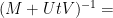

noting that the inverses here will exist for 
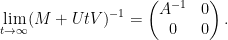
On the other hand, by the Woodbury matrix identity (discussed in this previous blog post), we have

and hence on taking limits and comparing with the preceding identity, one has

This achieves the aim of expressing the inverse

In the 

where 

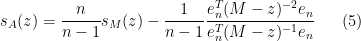
We can apply this identity to understand how the spectrum of an 

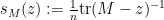

At this point we begin to proceed informally. Assume for sake of argument that the random matrix 


One can think of 


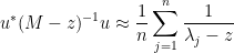
and thus

(that is to say, the diagonal entries of 
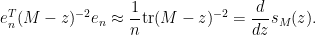
Inserting this into (5) and discarding terms of size 

This can be viewed as a difference equation for the Stieltjes transform of top left minors of 


where 

with initial data 
Example 1 If
of the identity, then
. One checks that
is a steady state solution to (7), which is unsurprising given that all minors of
times the identity.
Example 2 If
, then by the semi-circular law (see previous notes) one has
(using an appropriate branch of the square root). One can then verify the self-similar solution
to (7), which is consistent with the fact that a top
when
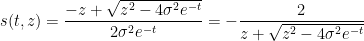
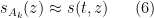
One can justify the approximation (6) given a sufficiently good well-posedness theory for the equation (7). We will not do so here, but will note that (as with the classical inviscid Burgers equation) the equation can be solved exactly (formally, at least) by the method of characteristics. For any initial position 

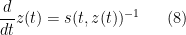
with initial data 

and thus 

and thus (7) may be solved implicitly via the equation

for all
Remark 3 In practice, the equation (9) may stop working when
crosses the real axis, as (7) does not necessarily hold in this region. It is a cute exercise (ultimately coming from the Cauchy-Schwarz inequality) to show that this crossing always happens, for instance if
necessarily has negative or zero imaginary part.
Example 4 Suppose we have
as in Example 1. Then (9) becomes
for any
, which after making the change of variables
becomes
as in Example 1.
Example 5 Suppose we have
as in Example 2. Then (9) becomes
If we write
one can calculate that
and hence


One can recover the spectral measure 


In this informal notation, we have for instance that

which can be interpreted as the fact that the Cauchy distributions 
If we let 


![{(0,1]}](https://s0.wp.com/latex.php?latex=%7B%280%2C1%5D%7D&bg=ffffff&fg=000000&s=0&c=20201002)


thus at height 
![{[-2\sigma \sqrt{\alpha}, 2\sigma \sqrt{\alpha}]}](https://s0.wp.com/latex.php?latex=%7B%5B-2%5Csigma+%5Csqrt%7B%5Calpha%7D%2C+2%5Csigma+%5Csqrt%7B%5Calpha%7D%5D%7D&bg=ffffff&fg=000000&s=0&c=20201002)


An interesting example of such a limiting Gelfand-Tsetlin pattern occurs when 


and so (9) in this case becomes
A tedious calculation then gives the solution
For 


This reflects the interlacing property, which forces 


For 

There is presumably a direct geometric explanation of this fact (basically describing the singular values of the product of two random orthogonal projections to half-dimensional subspaces of
The evolution of 


for all 
The equation (9) may be rewritten as

and hence


See these previous notes for a discussion of free probability topics such as the
Example 6 If
.
Example 7 If
Example 8 If

This simple relationship (12) is essentially due to Nica and Speicher (thanks to Dima Shylakhtenko for this reference). It has the remarkable consequence that when 


In a similar vein, if one defines the function

and inverts it to obtain a function 
for all 

Writing

for any

and so (9) becomes

which simplifies to
replacing 

and thus
and hence
One can compute 


Apoorva Khare and I have just uploaded to the arXiv our paper “On the sign patterns of entrywise positivity preservers in fixed dimension“. This paper explores the relationship between positive definiteness of Hermitian matrices, and entrywise operations on these matrices. The starting point for this theory is the Schur product theorem, which asserts that if 


is also positive semi-definite. (One should caution that the Hadamard product is not the same as the usual matrix product.) To prove this theorem, first observe that the claim is easy when 


One corollary of the Schur product theorem is that any polynomial 


![\displaystyle P[A] := (P(a_{ij}))_{1 \leq i,j \leq N}](https://s0.wp.com/latex.php?latex=%5Cdisplaystyle++P%5BA%5D+%3A%3D+%28P%28a_%7Bij%7D%29%29_%7B1+%5Cleq+i%2Cj+%5Cleq+N%7D&bg=ffffff&fg=000000&s=0&c=20201002)
of ![{P[A]}](https://s0.wp.com/latex.php?latex=%7BP%5BA%5D%7D&bg=ffffff&fg=000000&s=0&c=20201002)

![\displaystyle P[A] = c_0 A^{\circ 0} + c_1 A^{\circ 1} + \dots + c_d A^{\circ d},](https://s0.wp.com/latex.php?latex=%5Cdisplaystyle++P%5BA%5D+%3D+c_0+A%5E%7B%5Ccirc+0%7D+%2B+c_1+A%5E%7B%5Ccirc+1%7D+%2B+%5Cdots+%2B+c_d+A%5E%7B%5Ccirc+d%7D%2C&bg=ffffff&fg=000000&s=0&c=20201002)
where 

A slight variant of this argument, already observed by Pólya and Szegö in 1925, shows that if 


is a power series with non-negative coefficients 
![{I = [0,\rho]}](https://s0.wp.com/latex.php?latex=%7BI+%3D+%5B0%2C%5Crho%5D%7D&bg=ffffff&fg=000000&s=0&c=20201002)
In the work of Schoenberg and of Rudin, we have a converse: if 


This gives a satisfactory classification of functions 


The main result of this paper is that these sign conditions are the only constraints for entrywise positivity preserving power series. More precisely:
Theorem 1 For each
be a sign.
- Suppose that any negative sign
is preceded by at least
with
). Then, for any
, with each
having the sign of
, which is entrywise positivity preserving on
.
- Suppose in addition that any negative sign
with
). Then there exists a convergent power series (1) on
, with each
.
One can ask the same question with 

The heart of the proofs of these results is an analysis of the determinants ![{\mathrm{det} P[ {\bf u} {\bf u}^* ]}](https://s0.wp.com/latex.php?latex=%7B%5Cmathrm%7Bdet%7D+P%5B+%7B%5Cbf+u%7D+%7B%5Cbf+u%7D%5E%2A+%5D%7D&bg=ffffff&fg=000000&s=0&c=20201002)

![{P[uu^*]}](https://s0.wp.com/latex.php?latex=%7BP%5Buu%5E%2A%5D%7D&bg=ffffff&fg=000000&s=0&c=20201002)
where 

of the generalised Vandermonde determinant into the ordinary Vandermonde determinant

and a Schur polynomial 


If we allow the exponents
It remains to understand what happens for more general positive semi-definite matrices 

![{P[{\bf u} {\bf u}^*]}](https://s0.wp.com/latex.php?latex=%7BP%5B%7B%5Cbf+u%7D+%7B%5Cbf+u%7D%5E%2A%5D%7D&bg=ffffff&fg=000000&s=0&c=20201002)
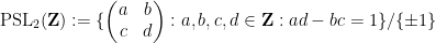
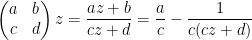
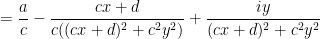
The Poincaré upper half-plane 


via fractional linear transformations:

Here and in the rest of the post we will abuse notation by identifying elements 


As the action of 

(using Cartesian coordinates 

the volume measure 

and the Laplace-Beltrami operator, which can be computed to be 

The Gauss curvature of the Poincaré half-plane can be computed to be the constant 


One can inject arithmetic into this geometric structure by passing from the Lie group
or congruence subgroups such as
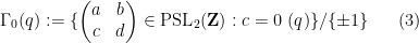
for natural number 

These are discrete subgroups of

There are many further discrete subgroups of
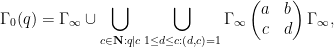
Any discrete subgroup 


For instance, a fundamental domain for 


![\displaystyle [\hbox{PSL}_2({\bf Z}) : \Gamma_0(q)] = q \prod_{p|q} (1 + \frac{1}{p}) = q^{1+o(1)}](https://s0.wp.com/latex.php?latex=%5Cdisplaystyle++%5B%5Chbox%7BPSL%7D_2%28%7B%5Cbf+Z%7D%29+%3A+%5CGamma_0%28q%29%5D+%3D+q+%5Cprod_%7Bp%7Cq%7D+%281+%2B+%5Cfrac%7B1%7D%7Bp%7D%29+%3D+q%5E%7B1%2Bo%281%29%7D+&bg=ffffff&fg=000000&s=0&c=20201002)
copies of a fundamental domain for
While fundamental domains can be a convenient choice of coordinates to work with for some computations (as well as for drawing appropriate pictures), it is geometrically more natural to avoid working explicitly on such domains, and instead work directly on the quotient spaces 


An important way to create a ![{P_\Gamma[f]: {\mathbf H} \rightarrow {\bf C}}](https://s0.wp.com/latex.php?latex=%7BP_%5CGamma%5Bf%5D%3A+%7B%5Cmathbf+H%7D+%5Crightarrow+%7B%5Cbf+C%7D%7D&bg=ffffff&fg=000000&s=0&c=20201002)
 = \sum_{\gamma \in \Gamma} f(\gamma z),](https://s0.wp.com/latex.php?latex=%5Cdisplaystyle++P_%7B%5CGamma%7D%5Bf%5D%28z%29+%3D+%5Csum_%7B%5Cgamma+%5Cin+%5CGamma%7D+f%28%5Cgamma+z%29%2C&bg=ffffff&fg=000000&s=0&c=20201002)
which is clearly 

![{P_{\Gamma_\infty \backslash \Gamma}[f]: {\mathbf H} \rightarrow {\bf C}}](https://s0.wp.com/latex.php?latex=%7BP_%7B%5CGamma_%5Cinfty+%5Cbackslash+%5CGamma%7D%5Bf%5D%3A+%7B%5Cmathbf+H%7D+%5Crightarrow+%7B%5Cbf+C%7D%7D&bg=ffffff&fg=000000&s=0&c=20201002)
 = \sum_{\gamma \in \hbox{Fund}(\Gamma_\infty \backslash \Gamma)} f(\gamma z)](https://s0.wp.com/latex.php?latex=%5Cdisplaystyle++P_%7B%5CGamma_%5Cinfty+%5Cbackslash+%5CGamma%7D%5Bf%5D%28z%29+%3D+%5Csum_%7B%5Cgamma+%5Cin+%5Chbox%7BFund%7D%28%5CGamma_%5Cinfty+%5Cbackslash+%5CGamma%29%7D+f%28%5Cgamma+z%29&bg=ffffff&fg=000000&s=0&c=20201002)
where 

![{P_{\Gamma_\infty \backslash \Gamma}[f]}](https://s0.wp.com/latex.php?latex=%7BP_%7B%5CGamma_%5Cinfty+%5Cbackslash+%5CGamma%7D%5Bf%5D%7D&bg=ffffff&fg=000000&s=0&c=20201002)
For future reference we record the basic but fundamental unfolding identities
![\displaystyle \int_{\Gamma \backslash {\mathbf H}} P_\Gamma[f] g\ d\mu_{\Gamma \backslash {\mathbf H}} = \int_{\mathbf H} f g\ d\mu_{\mathbf H} \ \ \ \ \ (5)](https://s0.wp.com/latex.php?latex=%5Cdisplaystyle++%5Cint_%7B%5CGamma+%5Cbackslash+%7B%5Cmathbf+H%7D%7D+P_%5CGamma%5Bf%5D+g%5C+d%5Cmu_%7B%5CGamma+%5Cbackslash+%7B%5Cmathbf+H%7D%7D+%3D+%5Cint_%7B%5Cmathbf+H%7D+f+g%5C+d%5Cmu_%7B%5Cmathbf+H%7D+%5C+%5C+%5C+%5C+%5C+%285%29&bg=ffffff&fg=000000&s=0&c=20201002)
for any function
![\displaystyle \int_{\Gamma \backslash {\mathbf H}} P_{\Gamma_\infty \backslash \Gamma}[f] g\ d\mu_{\Gamma \backslash {\mathbf H}} = \int_{\Gamma_\infty \backslash {\mathbf H}} f g\ d\mu_{\Gamma_\infty \backslash {\mathbf H}} \ \ \ \ \ (6)](https://s0.wp.com/latex.php?latex=%5Cdisplaystyle++%5Cint_%7B%5CGamma+%5Cbackslash+%7B%5Cmathbf+H%7D%7D+P_%7B%5CGamma_%5Cinfty+%5Cbackslash+%5CGamma%7D%5Bf%5D+g%5C+d%5Cmu_%7B%5CGamma+%5Cbackslash+%7B%5Cmathbf+H%7D%7D+%3D+%5Cint_%7B%5CGamma_%5Cinfty+%5Cbackslash+%7B%5Cmathbf+H%7D%7D+f+g%5C+d%5Cmu_%7B%5CGamma_%5Cinfty+%5Cbackslash+%7B%5Cmathbf+H%7D%7D+%5C+%5C+%5C+%5C+%5C+%286%29&bg=ffffff&fg=000000&s=0&c=20201002)
whenever 
When computing various statistics of a Poincaré series ![{P_\Gamma[f]}](https://s0.wp.com/latex.php?latex=%7BP_%5CGamma%5Bf%5D%7D&bg=ffffff&fg=000000&s=0&c=20201002)
}](https://s0.wp.com/latex.php?latex=%7BP_%5CGamma%5Bf%5D%28z%29%7D&bg=ffffff&fg=000000&s=0&c=20201002)
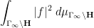
![{\int_{\Gamma \backslash {\mathbf H}} |P_\Gamma[f]|^2\ d\mu}](https://s0.wp.com/latex.php?latex=%7B%5Cint_%7B%5CGamma+%5Cbackslash+%7B%5Cmathbf+H%7D%7D+%7CP_%5CGamma%5Bf%5D%7C%5E2%5C+d%5Cmu%7D&bg=ffffff&fg=000000&s=0&c=20201002)
The first example we will give concerns the problem of estimating the sum
where 


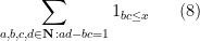
which is basically a sum over the full modular group 
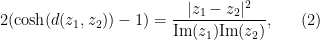
This sum is not exactly the same as (8), but will be a little easier to handle, and it is plausible that the methods used to handle this sum can be modified to handle (8). Observe from (2) and some calculation that the distance between 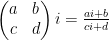
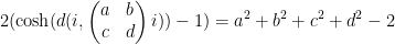
and so one can express the above sum as

(the factor of 

}](https://s0.wp.com/latex.php?latex=%7BP_%5CGamma%5Bf%5D%28i%29%7D&bg=ffffff&fg=000000&s=0&c=20201002)

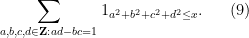
The second example concerns the relative

of the sum (7). Note from multiplicativity that (7) can be written as 

As with (7), we may expand (10) as
At first glance this does not look like a sum over a modular group, but one can manipulate this expression into such a form in one of two (closely related) ways. First, observe that any factorisation 


and one the modular group 


which (up to a harmless sign) is exactly the representation 

Note that 


Sums involving subgroups of the full modular group, such as 


The third and final example concerns averages of Kloosterman sums
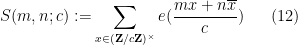
where 


![\displaystyle \int_{\Gamma_0(q) \backslash {\mathbf H}} |P_{\Gamma_\infty \backslash \Gamma_0(q)}[f]|^2\ d\mu_{\Gamma \backslash {\mathbf H}} \ \ \ \ \ (13)](https://s0.wp.com/latex.php?latex=%5Cdisplaystyle++%5Cint_%7B%5CGamma_0%28q%29+%5Cbackslash+%7B%5Cmathbf+H%7D%7D+%7CP_%7B%5CGamma_%5Cinfty+%5Cbackslash+%5CGamma_0%28q%29%7D%5Bf%5D%7C%5E2%5C+d%5Cmu_%7B%5CGamma+%5Cbackslash+%7B%5Cmathbf+H%7D%7D+%5C+%5C+%5C+%5C+%5C+%2813%29&bg=ffffff&fg=000000&s=0&c=20201002)
where

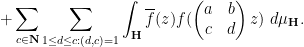
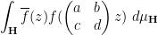
for some integer 
![\displaystyle \int_{\Gamma_\infty \backslash {\mathbf H}} \overline{f} P_{\Gamma_\infty \backslash \Gamma_0(q)}[f]\ d\mu_{\Gamma_\infty \backslash {\mathbf H}}.](https://s0.wp.com/latex.php?latex=%5Cdisplaystyle++%5Cint_%7B%5CGamma_%5Cinfty+%5Cbackslash+%7B%5Cmathbf+H%7D%7D+%5Coverline%7Bf%7D+P_%7B%5CGamma_%5Cinfty+%5Cbackslash+%5CGamma_0%28q%29%7D%5Bf%5D%5C+d%5Cmu_%7B%5CGamma_%5Cinfty+%5Cbackslash+%7B%5Cmathbf+H%7D%7D.&bg=ffffff&fg=000000&s=0&c=20201002)
To compute this, we use the double coset decomposition
where for each 


![{[1,c]}](https://s0.wp.com/latex.php?latex=%7B%5B1%2Cc%5D%7D&bg=ffffff&fg=000000&s=0&c=20201002)

![\displaystyle P_{\Gamma_\infty \backslash \Gamma_0(q)}[f] = f + \sum_{c \in {\mathbf N}: q|c} \sum_{1 \leq d \leq c: (d,c)=1} P_{\Gamma_\infty}[ f( \begin{pmatrix} a & b \\ c & d \end{pmatrix} \cdot ) ]](https://s0.wp.com/latex.php?latex=%5Cdisplaystyle++P_%7B%5CGamma_%5Cinfty+%5Cbackslash+%5CGamma_0%28q%29%7D%5Bf%5D+%3D+f+%2B+%5Csum_%7Bc+%5Cin+%7B%5Cmathbf+N%7D%3A+q%7Cc%7D+%5Csum_%7B1+%5Cleq+d+%5Cleq+c%3A+%28d%2Cc%29%3D1%7D+P_%7B%5CGamma_%5Cinfty%7D%5B+f%28+%5Cbegin%7Bpmatrix%7D+a+%26+b+%5C%5C+c+%26+d+%5Cend%7Bpmatrix%7D+%5Ccdot+%29+%5D&bg=ffffff&fg=000000&s=0&c=20201002)
and so from further use of the unfolding formula (5) we may expand (13) as
The first integral is just 
so we can write
as


which on shifting 


and then on scaling 

Note that as 
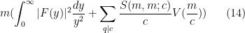
where

is a certain integral involving 

Traditionally, automorphic forms have been analysed using the spectral theory of the Laplace-Beltrami operator 


for 


However, as discussed in this previous post, the spectral theory of an essentially self-adjoint operator such as 


Actually it will be a bit more convenient to normalise the Laplacian by 

This equation somewhat resembles a “Klein-Gordon” type equation, except that the mass is imaginary! This would lead to pathological behaviour were it not for the negative curvature, which in principle creates a spectral gap of
The point is that the wave equation approach gives access to some nice PDE techniques, such as energy methods, Sobolev inequalities and finite speed of propagation, which are somewhat submerged in the spectral framework. The wave equation also interacts well with Poincaré series; if for instance ![{P_{\Gamma_\infty \backslash \Gamma}[u]}](https://s0.wp.com/latex.php?latex=%7BP_%7B%5CGamma_%5Cinfty+%5Cbackslash+%5CGamma%7D%5Bu%5D%7D&bg=ffffff&fg=000000&s=0&c=20201002)
![{P_{\Gamma_\infty \backslash \Gamma}[F]}](https://s0.wp.com/latex.php?latex=%7BP_%7B%5CGamma_%5Cinfty+%5Cbackslash+%5CGamma%7D%5BF%5D%7D&bg=ffffff&fg=000000&s=0&c=20201002)
- Using the Weil bound on Kloosterman sums to derive Selberg’s 3/16 theorem on the least non-trivial eigenvalue for
- Conversely, showing that Selberg’s eigenvalue conjecture (improving Selberg’s
bound to the optimal
) implies an optimal bound on (smoothed) sums of Kloosterman sums; and
- Using the same bound to obtain pointwise bounds on Poincaré series similar to the ones discussed above. (Actually, the argument here does not use the wave equation, instead it just uses the Sobolev inequality.)
This post originated from an attempt to finally learn this part of analytic number theory properly, and to see if I could use a PDE-based perspective to understand it better. Ultimately, this is not that dramatic a depature from the standard approach to this subject, but I found it useful to think of things in this fashion, probably due to my existing background in PDE.
I thank Bill Duke and Ben Green for helpful discussions. My primary reference for this theory was Chapters 15, 16, and 21 of Iwaniec and Kowalski.
Because of Euler’s identity 


![{(-\infty,0]}](https://s0.wp.com/latex.php?latex=%7B%28-%5Cinfty%2C0%5D%7D&bg=ffffff&fg=000000&s=0&c=20201002)
![{\hbox{Log}: {\bf C} \backslash (-\infty,0] \rightarrow \{ z \in {\bf C}: |\hbox{Im} z| < \pi \}}](https://s0.wp.com/latex.php?latex=%7B%5Chbox%7BLog%7D%3A+%7B%5Cbf+C%7D+%5Cbackslash+%28-%5Cinfty%2C0%5D+%5Crightarrow+%5C%7B+z+%5Cin+%7B%5Cbf+C%7D%3A+%7C%5Chbox%7BIm%7D+z%7C+%3C+%5Cpi+%5C%7D%7D&bg=ffffff&fg=000000&s=0&c=20201002)


- The standard branch
is holomorphic on its domain
.
- One has
for all
is real, then
is real.
- One has
for all
One can then also use the standard branch of the logarithm to create standard branches of other multi-valued functions, for instance creating a standard branch 

One can extend this standard branch of the logarithm to 


![{\lambda \in {\bf C} \backslash (-\infty,0]}](https://s0.wp.com/latex.php?latex=%7B%5Clambda+%5Cin+%7B%5Cbf+C%7D+%5Cbackslash+%28-%5Cinfty%2C0%5D%7D&bg=ffffff&fg=000000&s=0&c=20201002)


where 


The matrix standard branch of the logarithm has many pleasant and easily verified properties (often inherited from their scalar counterparts), whenever
- (i) We have
.
- (ii) If
and
have no spectrum in
.
- (iii) If
in
, where
is the Taylor series of
- (iv)
depends holomorphically on
for a contour
in the domain enclosing the spectrum of
- (v) If
is any invertible linear or antilinear map, then
. In particular, the standard branch of the logarithm commutes with matrix conjugations; and if
- (vi) If
denotes the transpose of
the complex dual of
. Similarly, if
denotes the adjoint of
the complex conjugate of
), then
.
- (vii) One has
.
- (viii) If
denotes the spectrum of
.
As a quick application of the standard branch of the matrix logarithm, we have
Proposition 1 Let
be one of the following matrix groups:
,
,
,
,
, or
, where
is a non-degenerate real quadratic form (so
for some
. Then any element
for some
in the Lie algebra
of
Proof: We just prove this for 


Exercise 2 Show that
is not exponential in
if
. Thus we see that the branch cut in the above proposition is largely necessary. See this paper of Djokovic for a more complete description of the image of the exponential map in classical groups, as well as this previous blog post for some more discussion of the surjectivity (or lack thereof) of the exponential map in Lie groups.
For a slightly less quick application of the standard branch, we have the following result (recently worked out in the answers to this MathOverflow question):
Proposition 3 Let
which lies in the connected component of the identity. Then
.
The requirement that 

Proof: We think of 


The spectrum of 


It remains to show that 


and so it suffices to show that 
At this point we need to use the hypothesis that 


We choose a complex basis of 


But since 


Hoi Nguyen, Van Vu, and myself have just uploaded to the arXiv our paper “Random matrices: tail bounds for gaps between eigenvalues“. This is a followup paper to my recent paper with Van in which we showed that random matrices 


for any
In the mean zero case, it becomes more efficient to use an inverse Littlewood-Offord theorem of Rudelson and Vershynin to obtain (with the normalisation that the entries of 

for 


for any fixed 

In the case of Erdös-Renyi graphs, we don’t have mean zero and the Rudelson-Vershynin Littlewood-Offord theorem isn’t quite applicable, but by working carefully through the approach based on the Nguyen-Vu theorem we can almost recover (1), except for a loss of 
As a sample applications of the eigenvalue separation results, we can now obtain some information about eigenvectors; for instance, we can show that the components of the eigenvectors all have magnitude at least
Van Vu and I have just uploaded to the arXiv our paper “Random matrices have simple spectrum“. Recall that an
For discrete random matrix ensembles, though, the above argument breaks down, even though general universality heuristics predict that the statistics of discrete ensembles should behave similarly to those of continuous ensembles. A model case here is the adjacency matrix 

Our argument works for more general Wigner-type matrix ensembles, but for sake of illustration we will stick with the Erdös-Renyi case. Previous work on local universality for such matrix models (e.g. the work of Erdos, Knowles, Yau, and Yin) was able to show that any individual eigenvalue gap 


Our argument in fact gives simplicity of the spectrum with probability 
The basic idea of argument can be sketched as follows. Suppose that

for a random 
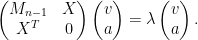
Extracting the top 
If we let 

we typically expect 

In other words, in order for
The prime number theorem can be expressed as the assertion

as 

is the von Mangoldt function. It is a basic result in analytic number theory, but requires a bit of effort to prove. One “elementary” proof of this theorem proceeds through the Selberg symmetry formula
where the second von Mangoldt function 


(We are avoiding the use of the 

suffices.
In this post I would like to record a somewhat “soft analysis” reformulation of the elementary proof of the prime number theorem in terms of Banach algebras, and specifically in Banach algebra structures on (completions of) the space 

This soft argument does not easily give any quantitative decay rate in the prime number theorem, but by the same token it avoids many of the quantitative calculations in the traditional proofs of this theorem. Ultimately, the key “soft analysis” fact used is the spectral radius formula

for any element 
The connection between prime numbers and Banach algebras is given by the following consequence of the Selberg symmetry formula.
Theorem 1 (Construction of a Banach algebra norm) For any
, let
denote the quantity
Then
is a seminorm on
for all
for all
.


We prove this theorem below the fold. The prime number theorem then follows from Theorem 1 and the following two assertions. The first is an application of the spectral radius formula (6) and some basic Fourier analysis (in particular, the observation that
Theorem 2 (Non-trivial Banach algebras with many local units have non-trivial spectrum) Let
such that
for all
. In particular, by (7), one has
whenever
is a non-negative function.


The second is a consequence of the Selberg symmetry formula and the fact that 


Theorem 3 (Breaking the parity barrier) Let

Assuming Theorems 1, 2, 3, we may now quickly establish the prime number theorem as follows. Theorem 2 and Theorem 3 imply that the seminorm

as 


as
as 
The same argument also yields the prime number theorem in arithmetic progressions, or equivalently that

for any fixed Dirichlet character 

In the traditional foundations of probability theory, one selects a probability space 


Actually, for our purposes we will adopt the philosophy of identifying stochastic objects that agree almost surely, so if one was to be completely precise, we should define a stochastic real number to be an equivalence class ![{[x]}](https://s0.wp.com/latex.php?latex=%7B%5Bx%5D%7D&bg=ffffff&fg=000000&s=0&c=20201002)
More generally, given any measurable space 


Remark 1 In my previous post on the foundations of probability theory, I emphasised the freedom to extend the sample space
Any (measurable) 

![{[x]+[y]}](https://s0.wp.com/latex.php?latex=%7B%5Bx%5D%2B%5By%5D%7D&bg=ffffff&fg=000000&s=0&c=20201002)


There is a similar story for 


Any universal identity for deterministic operations (or universal implication between identities) extends to their stochastic counterparts: for instance, addition is commutative, associative, and cancellative on the space of deterministic reals 


and then make all sets stochastic to obtain the true statement

thus we have to allow the index 


Similarly, the law of the excluded middle fails when interpreted deterministically, but remains true when interpreted stochastically: if
To avoid having to keep pointing out which operations are interpreted stochastically and which ones are interpreted deterministically, we will use the following convention: if we assert that a mathematical sentence 


In the above discussion, the stochastic objects 


Of course, in any reasonable application one can avoid the set theoretic issues at least by various ad hoc means, for instance by restricting the dimension of all spaces involved to some fixed cardinal such as 
In this post I would like to describe a different way to formalise stochastic spaces, and stochastic elements of these spaces, by viewing the spaces as measure-theoretic analogue of a sheaf, but being over the probability space 


The approach taken in this post is “topos-theoretic” in nature (although we will not use the language of topoi explicitly here), and is well suited to a “pointless” or “point-free” approach to probability theory, in which the role of the stochastic state
Definition 1 (Stochastic set) Unless otherwise specified, we assume that we are given a fixed finite measure space
(which we refer to as the base space). A stochastic set (relative to
consisting of the following objects:
- A set
assigned to each event
; and
- A restriction map
from
to
of nested events
. (Strictly speaking, one should indicate the dependence on
instead of
We refer to elements of
, localised to the event
Furthermore, we impose the following axioms:
- (Category) The map
are events in
for all
.
- (Null events trivial) If
is always a singleton set; this is analogous to the convention that
for any number
- (Countable gluing) Suppose that for each natural number
and an element
such that
for all
. Then there exists a unique
such that
for all
If
of the stochastic set
relative to

The following fact is useful for actually verifying that a given object indeed has the structure of a stochastic set:
Exercise 1 Show that to verify the countable gluing axiom of a stochastic set, it suffices to do so under the additional hypothesis that the events
are disjoint. (Note that this is quite different from the situation with sheaves over a topological space, in which the analogous gluing axiom is often trivial in the disjoint case but has non-trivial content in the overlapping case. This is ultimately because a
Let us illustrate the concept of a stochastic set with some examples.
Example 1 (Discrete case) A simple case arises when
to each
. One then sets
, with the obvious restriction maps, giving rise to a stochastic set
on
.) Conversely, it is not difficult to see that any stochastic set over an at most countable discrete probability space
Example 2 (Measurable spaces as stochastic sets) Returning now to a general base space
, together with the quotienting by almost sure equivalence, means that
of fibres, but this still serves as a useful first approximation to what
Example 3 (Extended Hilbert modules) This example is the one that motivated this post for me. Suppose that one has an extension
of the base space
, thus we have a measurable factor map
such that the pushforward of the measure
by
, defined as the adjoint of the pullback map
. As is well known, the conditional expectation operator also extends to a contraction
; by monotone convergence we may also extend
to a map from measurable functions from
to the extended non-negative reals
, to measurable functions from
to be the space of functions
with
finite almost everywhere. This is an extended version of the Hilbert module
, which is defined similarly except that
; this is a Hilbert module over
which is of particular importance in the Furstenberg-Zimmer structure theory of measure-preserving systems. We can then define the stochastic set
by setting
with the obvious restriction maps. In the case that
are standard Borel spaces, one can disintegrate
as an integral
of probability measures
(supported in the fibre
), in which case this stochastic set can be viewed as having fibres
(though if

We make the remark that if 

As a corollary of the above observation, we see that if the base space
Exercise 2 If
for
One can now start take many of the fundamental objects, operations, and results in set theory (and, hence, in most other categories of mathematics) and establish analogues relative to a finite measure space. Implicitly, what we will be doing in the next few paragraphs is endowing the category of stochastic sets with the structure of an elementary topos. However, to keep things reasonably concrete, we will not explicitly emphasise the topos-theoretic formalism here, although it is certainly lurking in the background.
Firstly, we define a stochastic function 


Thus (in the discrete, at most countable setting, at least) stochastic functions do not mix together information from different states 
One can now form the stochastic set 


In a similar spirit, we say that one stochastic set 


Note that if 


In a similar spirit, if 


Remark 2 One should caution that in the definition of the subset relation
.
Now we discuss Boolean operations on stochastic subsets of a given stochastic set 


This is easily verified to again be a stochastic subset of 

Stochastic unions are a bit more subtle. The set 


One can also consider a stochastic finite union 


The Cartesian product 


Remark 3 In the degenerate case when
), and any two deterministic objects
.
The following simple observation is crucial to subsequent discussion. If 


We now specialise from the extremely broad discipline of set theory to the more focused discipline of real analysis. There are two fundamental axioms that underlie real analysis (and in particular distinguishes it from real algebra). The first is the Archimedean property, which we phrase in the “no infinitesimal” formulation as follows:
Proposition 2 (Archimedean property) Let
for all positive natural numbers
.
The other is the least upper bound axiom:
Proposition 3 (Least upper bound axiom) Let
, thus
for all
. Then there exists a unique real number
with the following properties:
for all
- For any real
, there exists
.
.
Furthermore,
does not depend on the choice of
The Archimedean property extends easily to the stochastic setting:
Proposition 4 (Stochastic Archimedean property) Let
be such that
Remark 4 Here, incidentally, is one place in which this stochastic formalism deviates from the nonstandard analysis formalism, as the latter certainly permits the existence of infinitesimal elements. On the other hand, we caution that stochastic real numbers are permitted to be unbounded, so that formulation of Archimedean property is not valid in the stochastic setting.
The proof is easy and is left to the reader. The least upper bound axiom also extends nicely to the stochastic setting, but the proof requires more work (in particular, our argument uses the monotone convergence theorem):
Theorem 5 (Stochastic least upper bound axiom) Let
be a stochastic subset of
which has a global upper bound
, thus
, and is globally non-empty in the sense that there is at least one global element
with the following properties:
- For any stochastic real
Furthermore,
For future reference, we note that the same result holds with 


Proof: Uniqueness is clear (using the Archimedean property), as well as the independence on 


We observe that 


Let 

then (by Proposition 3!) 

Using the lattice property, we may assume that the 


If 

From this and (1) we conclude that

From monotone convergence, we conclude that

and so
Now let 


Remark 5 One can abstract away the role of the measure
Using Proposition 4 and Theorem 5, one can then revisit many of the other foundational results of deterministic real analysis, and develop stochastic analogues; we give some examples of this below the fold (focusing on the Heine-Borel theorem and a case of the spectral theorem). As an application of this formalism, we revisit some of the Furstenberg-Zimmer structural theory of measure-preserving systems, particularly that of relatively compact and relatively weakly mixing systems, and interpret them in this framework, basically as stochastic versions of compact and weakly mixing systems (though with the caveat that the shift map is allowed to act non-trivially on the underlying probability space). As this formalism is “point-free”, in that it avoids explicit use of fibres and disintegrations, it will be well suited for generalising this structure theory to settings in which the underlying probability spaces are not standard Borel, and the underlying groups are uncountable; I hope to discuss such generalisations in future blog posts.
Remark 6 Roughly speaking, stochastic real analysis can be viewed as a restricted subset of classical real analysis in which all operations have to be “measurable” with respect to the base space. In particular, indiscriminate application of the axiom of choice is not permitted, and one should largely restrict oneself to performing countable unions and intersections rather than arbitrary unions or intersections. Presumably one can formalise this intuition with a suitable “countable transfer principle”, but I was not able to formulate a clean and general principle of this sort, instead verifying various assertions about stochastic objects by hand rather than by direct transfer from the deterministic setting. However, it would be desirable to have such a principle, since otherwise one is faced with the tedious task of redoing all the foundations of real analysis (or whatever other base theory of mathematics one is going to be working in) in the stochastic setting by carefully repeating all the arguments.
More generally, topos theory is a good formalism for capturing precisely the informal idea of performing mathematics with certain operations, such as the axiom of choice, the law of the excluded middle, or arbitrary unions and intersections, being somehow “prohibited” or otherwise “restricted”.
One of the basic tools in modern combinatorics is the probabilistic method, introduced by Erdos, in which a deterministic solution to a given problem is shown to exist by constructing a random candidate for a solution, and showing that this candidate solves all the requirements of the problem with positive probability. When the problem requires a real-valued statistic
Proposition 1 (Comparison with mean) Let
is finite. Then
with positive probability, and
with positive probability.


This proposition is usually applied in conjunction with a computation of the first moment
As a typical example in random matrix theory, if one wanted to understand how small or how large the operator norm 


Recently, in their proof of the Kadison-Singer conjecture (and also in their earlier paper on Ramanujan graphs), Marcus, Spielman, and Srivastava introduced an striking new variant of the first moment method, suited in particular for controlling the operator norm 


where 

Prior to the work of Marcus, Spielman, and Srivastava, I think it is safe to say that the conventional wisdom in random matrix theory was that the representation (1) of the operator norm 


Proposition 2 (Comparison with mean) Let
. Let
of independent Hermitian rank one
, each taking a finite number of values. Then
with positive probability, and
with positive probability.


We prove this proposition below the fold. The hypothesis that each 

Proposition 3 (Deterministic multilinearisation formula) Let
for all
, where the mixed characteristic polynomial
of any
 \ \ \ \ \ (2)](https://s0.wp.com/latex.php?latex=%5Cdisplaystyle++p_A%28z%29+%3D+%5Cmu%5BA_1%2C%5Cldots%2CA_m%5D%28z%29+%5C+%5C+%5C+%5C+%5C+%282%29&bg=ffffff&fg=000000&s=0&c=20201002)
 \ \ \ \ \ (3)](https://s0.wp.com/latex.php?latex=%5Cdisplaystyle++%5Cmu%5BA_1%2C%5Cldots%2CA_m%5D%28z%29+%5C+%5C+%5C+%5C+%5C+%283%29&bg=ffffff&fg=000000&s=0&c=20201002)
Among other things, this formula gives a useful representation of the mean characteristic polynomial 
Corollary 4 (Random multilinearisation formula) Let
for all
.
 \ \ \ \ \ (4)](https://s0.wp.com/latex.php?latex=%5Cdisplaystyle++%5Cmathop%7B%5Cbf+E%7D+p_A%28z%29+%3D+%5Cmu%5B+%5Cmathop%7B%5Cbf+E%7D+A_1%2C+%5Cldots%2C+%5Cmathop%7B%5Cbf+E%7D+A_m+%5D%28z%29+%5C+%5C+%5C+%5C+%5C+%284%29&bg=ffffff&fg=000000&s=0&c=20201002)
Proof: For fixed 


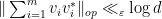
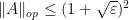
In view of Proposition 2, we can now hope to control the operator norm
Theorem 5 (Marcus-Spielman-Srivastava theorem) Let
be jointly independent random vectors in
, with each
taking a finite number of values. Suppose that we have the normalisation
where we are using the convention that
for some
. Then one has
with positive probability.


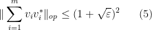
Note that the upper bound in (5) must be at least 


In the paper of Marcus, Spielman and Srivastava, Theorem 5 is used to deduce a conjecture 
Let us now summarise how Theorem 5 is proven. In the spirit of semi-definite programming, we rephrase the above theorem in terms of the rank one Hermitian positive semi-definite matrices 
Theorem 6 (Marcus-Spielman-Srivastava theorem again) Let
has mean
and such that
for some
with positive probability.


In view of (1) and Proposition 2, this theorem follows from the following control on the mean characteristic polynomial:
Theorem 7 (Control of mean characteristic polynomial) Let
and such that
for some


This result is proven using the multilinearisation formula (Corollary 4) and some convexity properties of real stable polynomials; we give the proof below the fold.
Thanks to Adam Marcus, Assaf Naor and Sorin Popa for many useful explanations on various aspects of the Kadison-Singer problem.

Recent Comments