Talks at the JMM

Earlier this year, I gave a series of lectures at the Joint Mathematics Meetings at San Francisco. I am uploading here the slides for these talks:

• “Machine assisted proof” (Video here)
• “Translational tilings of Euclidean space” (Video here)
• “Correlations of multiplicative functions” (Video here)

I also have written a text version of the first talk, which has been submitted to the Notices of the American Mathematical Society.

Monotone non-decreasing sequences of the Euler totient function

I have just uploaded to the arXiv my paper “Monotone non-decreasing sequences of the Euler totient function“. This paper concerns the quantity , defined as the length of the longest subsequence of the numbers from to for which the Euler totient function is non-decreasing. The first few values of are

(OEIS A365339). For instance, because the totient function is non-decreasing on the set or , but not on the set .

Since for any prime , we have , where is the prime counting function. Empirically, the primes come quite close to achieving the maximum length ; indeed it was conjectured by Pollack, Pomerance, and Treviño, based on numerical evidence, that one had

for all ; this conjecture is verified up to . The previous best known upper bound was basically of the form

as for an explicit constant , from combining results from the above paper with that of Ford or of Maier-Pomerance. In this paper we obtain the asymptotic

so in particular . This answers a question of Erdős, as well as a closely related question of Pollack, Pomerance, and Treviño.

The methods of proof turn out to be mostly elementary (the most advanced result from analytic number theory we need is the prime number theorem with classical error term). The basic idea is to isolate one key prime factor of a given number which has a sizeable influence on the totient function . For instance, for “typical” numbers , one has a factorization

where is a medium sized prime, is a significantly larger prime, and is a number with all prime factors less than . This leads to an approximation

As a consequence, if we temporarily hold fixed, and also localize to a relatively short interval, then can only be non-decreasing in if is also non-decreasing at the same time. This turns out to significantly cut down on the possible length of a non-decreasing sequence in this regime, particularly if is large; this can be formalized by partitioning the range of into various subintervals and inspecting how this (and the monotonicity hypothesis on ) constrains the values of associated to each subinterval. When is small, we instead use a factorization

where is very smooth (i.e., has no large prime factors), and is a large prime. Now we have the approximation

and we can conclude that will have to basically be piecewise constant in order for to be non-decreasing. Pursuing this analysis more carefully (in particular controlling the size of various exceptional sets in which the above analysis breaks down), we end up achieving the main theorem so long as we can prove the preliminary inequality

for all positive rational numbers . This is in fact also a necessary condition; any failure of this inequality can be easily converted to a counterexample to the bound (2), by considering numbers of the form (3) with equal to a fixed constant (and omitting a few rare values of where the approximation (4) is bad enough that is temporarily decreasing). Fortunately, there is a minor miracle, relating to the fact that the largest prime factor of denominator of in lowest terms necessarily equals the largest prime factor of , that allows one to evaluate the left-hand side of (5) almost exactly (this expression either vanishes, or is the product of for some primes ranging up to the largest prime factor of ) that allows one to easily establish (5). If one were to try to prove an analogue of our main result for the sum-of-divisors function , one would need the analogue

of (5), which looks within reach of current methods (and was even claimed without proof by Erdos), but does not have a full proof in the literature at present.

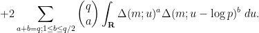
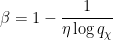
In the final section of the paper we discuss some near counterexamples to the strong conjecture (1) that indicate that it is likely going to be difficult to get close to proving this conjecture without assuming some rather strong hypotheses. Firstly, we show that failure of Legendre’s conjecture on the existence of a prime between any two consecutive squares can lead to a counterexample to (1). Secondly, we show that failure of the Dickson-Hardy-Littlewood conjecture can lead to a separate (and more dramatic) failure of (1), in which the primes are no longer the dominant sequence on which the totient function is non-decreasing, but rather the numbers which are a power of two times a prime become the dominant sequence. This suggests that any significant improvement to (2) would require assuming something comparable to the prime tuples conjecture, and perhaps also some unproven hypotheses on prime gaps.

A lower bound on the mean value of the Erdős-Hooley delta function

Kevin Ford, Dimitris Koukoulopoulos and I have just uploaded to the arXiv our paper “A lower bound on the mean value of the Erdős-Hooley delta function“. This paper complements the recent paper of Dimitris and myself obtaining the upper bound

on the mean value of the Erdős-Hooley delta function

In this paper we obtain a lower bound

where is an exponent that arose in previous work of result of Ford, Green, and Koukoulopoulos, who showed that

for all outside of a set of density zero. The previous best known lower bound for the mean value was

due to Hall and Tenenbaum.

The point is the main contributions to the mean value of are driven not by “typical” numbers of some size , but rather of numbers that have a splitting

where is the product of primes between some intermediate threshold and and behaves “typically” (so in particular, it has about prime factors, as per the Hardy-Ramanujan law and the Erdős-Kac law, but is the product of primes up to and has double the number of typical prime factors – , rather than – thus is the type of number that would make a significant contribution to the mean value of the divisor function . Here is such that is an integer in the range

for some small constant there are basically different values of give essentially disjoint contributions. From the easy inequalities

(the latter coming from the pigeonhole principle) and the fact that has mean about one, one would expect to get the above result provided that one could get a lower bound of the form

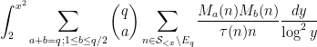
for most typical with prime factors between and . Unfortunately, due to the lack of small prime factors in , the arguments of Ford, Green, Koukoulopoulos that give (1) for typical do not quite work for the rougher numbers . However, it turns out that one can get around this problem by replacing (2) by the more efficient inequality

where

is an enlarged version of when . This inequality is easily proven by applying the pigeonhole principle to the factors of of the form , where is one of the factors of , and is one of the factors of in the optimal interval . The extra room provided by the enlargement of the range to turns out to be sufficient to adapt the Ford-Green-Koukoulopoulos argument to the rough setting. In fact we are able to use the main technical estimate from that paper as a “black box”, namely that if one considers a random subset of for some small and sufficiently large with each lying in with an independent probability , then with high probability there should be subset sums of that attain the same value. (Initially, what “high probability” means is just “close to “, but one can reduce the failure probability significantly as by a “tensor power trick” taking advantage of Bennett’s inequality.)

The convergence of an alternating series of Erdős, assuming the Hardy–Littlewood prime tuples conjecture

I have just uploaded to the arXiv my paper “The convergence of an alternating series of Erdős, assuming the Hardy–Littlewood prime tuples conjecture“. This paper concerns an old problem of Erdős concerning whether the alternating series converges, where denotes the prime. The main result of this paper is that the answer to this question is affirmative assuming a sufficiently strong version of the Hardy–Littlewood prime tuples conjecture.

The alternating series test does not apply here because the ratios are not monotonically decreasing. The deviations of monotonicity arise from fluctuations in the prime gaps , so the enemy arises from biases in the prime gaps for odd and even . By changing variables from to (or more precisely, to integers in the range between and ), this is basically equivalent to biases in the parity of the prime counting function. Indeed, it is an unpublished observation of Said that the convergence of is equivalent to the convergence of . So this question is really about trying to get a sufficiently strong amount of equidistribution for the parity of .

The prime tuples conjecture does not directly say much about the value of ; however, it can be used to control differences for and not too large. Indeed, it is a famous calculation of Gallagher that for fixed , and chosen randomly from to , the quantity is distributed according to the Poisson distribution of mean asymptotically if the prime tuples conjecture holds. In particular, the parity of this quantity should have mean asymptotic to . An application of the van der Corput -process then gives some decay on the mean of as well. Unfortunately, this decay is a bit too weak for this problem; even if one uses the most quantitative version of Gallagher’s calculation, worked out in a recent paper of (Vivian) Kuperberg, the best bound on the mean is something like , which is not quite strong enough to overcome the doubly logarithmic divergence of .

To get around this obstacle, we take advantage of the random sifted model of the primes that was introduced in a paper of Banks, Ford, and myself. To model the primes in an interval such as with drawn randomly from say , we remove one random residue class from this interval for all primes up to Pólya’s “magic cutoff” . The prime tuples conjecture can then be intepreted as the assertion that the random set produced by this sieving process is statistically a good model for the primes in . After some standard manipulations (using a version of the Bonferroni inequalities, as well as some upper bounds of Kuperberg), the problem then boils down to getting sufficiently strong estimates for the expected parity of the random sifted set .

For this problem, the main advantage of working with the random sifted model, rather than with the primes or the singular series arising from the prime tuples conjecture, is that the sifted model can be studied iteratively from the partially sifted sets arising from sifting primes up to some intermediate threshold , and that the expected parity of the experiences some decay in . Indeed, once exceeds the length of the interval , sifting by an additional prime will cause to lose one element with probability , and remain unchanged with probability . If concentrates around some value , this suggests that the expected parity will decay by a factor of about as one increases to , and iterating this should give good bounds on the final expected parity . It turns out that existing second moment calculations of Montgomery and Soundararajan suffice to obtain enough concentration to make this strategy work.

An upper bound on the mean value of the Erdős-Hooley delta function

Dimitris Koukoulopoulos and I have just uploaded to the arXiv our paper “An upper bound on the mean value of the Erdős-Hooley delta function“. This paper concerns a (still somewhat poorly understood) basic arithmetic function in multiplicative number theory, namely the Erdos-Hooley delta function

where

The function measures the extent to which the divisors of a natural number can be concentrated in a dyadic (or more precisely, -dyadic) interval . From the pigeonhole principle, we have the bounds

where is the usual divisor function. The statistical behavior of the divisor function is well understood; for instance, if is drawn at random from to , then the mean value of is roughly , the median is roughly , and (by the Erdős-Kac theorem) asymptotically has a log-normal distribution. In particular, there are a small proportion of highly divisible numbers that skew the mean to be significantly higher than the median.

On the other hand, the statistical behavior of the Erdős-Hooley delta function is significantly less well understood, even conjecturally. Again drawing at random from to for large , the median is known to be somewhere between and for large – a (difficult) recent result of Ford, Green, and Koukoulopolous (for the lower bound) and La Bretèche and Tenenbaum (for the upper bound). And the mean was even less well controlled; the best previous bounds were

for any , with the lower bound due to Hall and Tenenbaum, and the upper bound a recent result of La Bretèche and Tenenbaum.

The main result of this paper is an improvement of the upper bound to

It is still unclear to us exactly what to conjecture regarding the actual order of the mean value.

The reason we looked into this problem was that it was connected to forthcoming work of David Conlon, Jacob Fox, and Huy Pham on the following problem of Erdos: what is the size of the largest subset of with the property that no non-empty subset of sums to a perfect square? Erdos observed that one can obtain sets of size (basically by considering certain homogeneous arithmetic progressions), and Nguyen and Vu showed an upper bound of . With our mean value bound as input, together with several new arguments, Conlon, Fox, and Pham have been able to improve the upper bound to .

Let me now discuss some of the ingredients of the proof. The first few steps are standard. Firstly we may restrict attention to square-free numbers without much difficulty (the point being that if a number factors as with squarefree, then ). Next, because a square-free number can be uniquely factored as where is a prime and lies in the finite set of squarefree numbers whose prime factors are less than , and , it is not difficult to establish the bound

The upshot of this is that one can replace an ordinary average with a logarithmic average, thus it suffices to show

We actually prove a slightly more refined distributional estimate: for any , we have a bound

outside of an exceptional set which is small in the sense that

It is not difficult to get from this distributional estimate to the logarithmic average estimate (1) (worsening the exponent to ).

To get some intuition on the size of , we observe that if and is the factor of coming from the prime factors less than , then

On the other hand, standard estimates let one establish that

for all , and all outside of an exceptional set that is small in the sense (3); in fact it turns out that one can also get an additional gain in this estimate unless is close to , which turns out to be useful when optimizing the bounds. So we would like to approximately reverse the inequalities in (4) and get from (5) to (2), possibly after throwing away further exceptional sets of size (3).

At this point we perform another standard technique, namely the moment method of controlling the supremum by the moments

for natural numbers ; it is not difficult to establish the bound

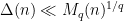
and one expects this bound to become essentially sharp once . We will be able to show a moment bound

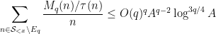
for any for some exceptional set obeying the smallness condition (3) (actually, for technical reasons we need to improve the right-hand side slightly to close an induction on ); this will imply the distributional bound (2) from a standard Markov inequality argument (setting ).

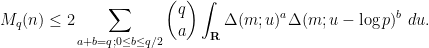
The strategy is then to obtain a good recursive inequality for (averages of) . As in the reduction to (1), we factor where is a prime and . One observes the identity

for any ; taking moments, one obtains the identity

As in previous literature, one can try to average in here and apply Hölder’s inequality. But it convenient to first use the symmetry of the summand in to reduce to the case of relatively small values of :

One can extract out the term as

It is convenient to eliminate the factor of by dividing out by the divisor function:

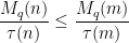
This inequality is suitable for iterating and also averaging in and . After some standard manipulations (using the Brun–Titchmarsh and Hölder inequalities), one is able to estimate sums such as

in terms of sums such as

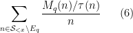
(assuming a certain monotonicity property of the exceptional set that turns out to hold in our application). By an induction hypothesis and a Markov inequality argument, one can get a reasonable pointwise upper bound on (after removing another exceptional set), and the net result is that one can basically control the sum (6) in terms of expressions such as

for various . This allows one to estimate these expressions efficiently by induction.

Infinite partial sumsets in the primes

Tamar Ziegler and I have just uploaded to the arXiv our paper “Infinite partial sumsets in the primes“. This is a short paper inspired by a recent result of Kra, Moreira, Richter, and Robertson (discussed for instance in this Quanta article from last December) showing that for any set of natural numbers of positive upper density, there exists a sequence of natural numbers and a shift such that for all this answers a question of Erdős). In view of the “transference principle“, it is then plausible to ask whether the same result holds if is replaced by the primes. We can show the following results:

Theorem 1

• (i) If the Hardy-Littlewood prime tuples conjecture (or the weaker conjecture of Dickson) is true, then there exists an increasing sequence of primes such that is prime for all .
• (ii) Unconditionally, there exist increasing sequences and of natural numbers such that is prime for all .
• (iii) These conclusions fail if “prime” is replaced by “positive (relative) density subset of the primes” (even if the density is equal to 1).

We remark that it was shown by Balog that there (unconditionally) exist arbitrarily long but finite sequences of primes such that is prime for all . (This result can also be recovered from the later results of Ben Green, myself, and Tamar Ziegler.) Also, it had previously been shown by Granville that on the Hardy-Littlewood prime tuples conjecture, there existed increasing sequences and of natural numbers such that is prime for all .

The conclusion of (i) is stronger than that of (ii) (which is of course consistent with the former being conditional and the latter unconditional). The conclusion (ii) also implies the well-known theorem of Maynard that for any given , there exist infinitely many -tuples of primes of bounded diameter, and indeed our proof of (ii) uses the same “Maynard sieve” that powers the proof of that theorem (though we use a formulation of that sieve closer to that in this blog post of mine). Indeed, the failure of (iii) basically arises from the failure of Maynard’s theorem for dense subsets of primes, simply by removing those clusters of primes that are unusually closely spaced.

Our proof of (i) was initially inspired by the topological dynamics methods used by Kra, Moreira, Richter, and Robertson, but we managed to condense it to a purely elementary argument (taking up only half a page) that makes no reference to topological dynamics and builds up the sequence recursively by repeated application of the prime tuples conjecture.

The proof of (ii) takes up the majority of the paper. It is easiest to phrase the argument in terms of “prime-producing tuples” – tuples for which there are infinitely many with all prime. Maynard’s theorem is equivalent to the existence of arbitrarily long prime-producing tuples; our theorem is equivalent to the stronger assertion that there exist an infinite sequence such that every initial segment is prime-producing. The main new tool for achieving this is the following cute measure-theoretic lemma of Bergelson:

Lemma 2 (Bergelson intersectivity lemma) Let be subsets of a probability space of measure uniformly bounded away from zero, thus . Then there exists a subsequence such that

for all .

This lemma has a short proof, though not an entirely obvious one. Firstly, by deleting a null set from , one can assume that all finite intersections are either positive measure or empty. Secondly, a routine application of Fatou’s lemma shows that the maximal function has a positive integral, hence must be positive at some point . Thus there is a subsequence whose finite intersections all contain , thus have positive measure as desired by the previous reduction.

It turns out that one cannot quite combine the standard Maynard sieve with the intersectivity lemma because the events that show up (which roughly correspond to the event that is prime for some random number (with a well-chosen probability distribution) and some shift ) have their probability going to zero, rather than being uniformly bounded from below. To get around this, we borrow an idea from a paper of Banks, Freiberg, and Maynard, and group the shifts into various clusters , chosen in such a way that the probability that at least one of is prime is bounded uniformly from below. One then applies the Bergelson intersectivity lemma to those events and uses many applications of the pigeonhole principle to conclude.

Higher uniformity of arithmetic functions in short intervals I. All intervals

Kaisa Matomäki, Xuancheng Shao, Joni Teräväinen, and myself have just uploaded to the arXiv our preprint “Higher uniformity of arithmetic functions in short intervals I. All intervals“. This paper investigates the higher order (Gowers) uniformity of standard arithmetic functions in analytic number theory (and specifically, the Möbius function , the von Mangoldt function , and the generalised divisor functions ) in short intervals , where is large and lies in the range for a fixed constant (that one would like to be as small as possible). If we let denote one of the functions , then there is extensive literature on the estimation of short sums

and some literature also on the estimation of exponential sums such as

for a real frequency , where . For applications in the additive combinatorics of such functions , it is also necessary to consider more general correlations, such as polynomial correlations

where is a polynomial of some fixed degree, or more generally

where is a nilmanifold of fixed degree and dimension (and with some control on structure constants), is a polynomial map, and is a Lipschitz function (with some bound on the Lipschitz constant). Indeed, thanks to the inverse theorem for the Gowers uniformity norm, such correlations let one control the Gowers uniformity norm of (possibly after subtracting off some renormalising factor) on such short intervals , which can in turn be used to control other multilinear correlations involving such functions.

Traditionally, asymptotics for such sums are expressed in terms of a “main term” of some arithmetic nature, plus an error term that is estimated in magnitude. For instance, a sum such as would be approximated in terms of a main term that vanished (or is negligible) if is “minor arc”, but would be expressible in terms of something like a Ramanujan sum if was “major arc”, together with an error term. We found it convenient to cancel off such main terms by subtracting an approximant from each of the arithmetic functions and then getting upper bounds on remainder correlations such as

(actually for technical reasons we also allow the variable to be restricted further to a subprogression of , but let us ignore this minor extension for this discussion). There is some flexibility in how to choose these approximants, but we eventually found it convenient to use the following choices.

• For the Möbius function , we simply set , as per the Möbius pseudorandomness conjecture. (One could choose a more sophisticated approximant in the presence of a Siegel zero, as I did with Joni in this recent paper, but we do not do so here.)
• For the von Mangoldt function , we eventually went with the Cramér-Granville approximant , where and .
• For the divisor functions , we used a somewhat complicated-looking approximant for some explicit polynomials , chosen so that and have almost exactly the same sums along arithmetic progressions (see the paper for details).

The objective is then to obtain bounds on sums such as (1) that improve upon the “trivial bound” that one can get with the triangle inequality and standard number theory bounds such as the Brun-Titchmarsh inequality. For and , the Siegel-Walfisz theorem suggests that it is reasonable to expect error terms that have “strongly logarithmic savings” in the sense that they gain a factor of over the trivial bound for any ; for , the Dirichlet hyperbola method suggests instead that one has “power savings” in that one should gain a factor of over the trivial bound for some . In the case of the Möbius function , there is an additional trick (introduced by Matomäki and Teräväinen) that allows one to lower the exponent somewhat at the cost of only obtaining “weakly logarithmic savings” of shape for some small .

Our main estimates on sums of the form (1) work in the following ranges:

• For , one can obtain strongly logarithmic savings on (1) for , and power savings for .
• For , one can obtain weakly logarithmic savings for .
• For , one can obtain power savings for .
• For , one can obtain power savings for .

Conjecturally, one should be able to obtain power savings in all cases, and lower down to zero, but the ranges of exponents and savings given here seem to be the limit of current methods unless one assumes additional hypotheses, such as GRH. The result for correlation against Fourier phases was established previously by Zhan, and the result for such phases and was established previously by by Matomäki and Teräväinen.

By combining these results with tools from additive combinatorics, one can obtain a number of applications:

• Direct insertion of our bounds in the recent work of Kanigowski, Lemanczyk, and Radziwill on the prime number theorem on dynamical systems that are analytic skew products gives some improvements in the exponents there.
• We can obtain a “short interval” version of a multiple ergodic theorem along primes established by Frantzikinakis-Host-Kra and Wooley-Ziegler, in which we average over intervals of the form rather than .
• We can obtain a “short interval” version of the “linear equations in primes” asymptotics obtained by Ben Green, Tamar Ziegler, and myself in this sequence of papers, where the variables in these equations lie in short intervals rather than long intervals such as .

We now briefly discuss some of the ingredients of proof of our main results. The first step is standard, using combinatorial decompositions (based on the Heath-Brown identity and (for the result) the Ramaré identity) to decompose into more tractable sums of the following types:

• Type sums, which are basically of the form for some weights of controlled size and some cutoff that is not too large;
• Type sums, which are basically of the form for some weights , of controlled size and some cutoffs that are not too close to or to ;
• Type sums, which are basically of the form for some weights of controlled size and some cutoff that is not too large.

The precise ranges of the cutoffs depend on the choice of ; our methods fail once these cutoffs pass a certain threshold, and this is the reason for the exponents being what they are in our main results.

The Type sums involving nilsequences can be treated by methods similar to those in this previous paper of Ben Green and myself; the main innovations are in the treatment of the Type and Type sums.

For the Type sums, one can split into the “abelian” case in which (after some Fourier decomposition) the nilsequence is basically of the form , and the “non-abelian” case in which is non-abelian and exhibits non-trivial oscillation in a central direction. In the abelian case we can adapt arguments of Matomaki and Shao, which uses Cauchy-Schwarz and the equidistribution properties of polynomials to obtain good bounds unless is “major arc” in the sense that it resembles (or “pretends to be”) for some Dirichlet character and some frequency , but in this case one can use classical multiplicative methods to control the correlation. It turns out that the non-abelian case can be treated similarly. After applying Cauchy-Schwarz, one ends up analyzing the equidistribution of the four-variable polynomial sequence

as range in various dyadic intervals. Using the known multidimensional equidistribution theory of polynomial maps in nilmanifolds, one can eventually show in the non-abelian case that this sequence either has enough equidistribution to give cancellation, or else the nilsequence involved can be replaced with one from a lower dimensional nilmanifold, in which case one can apply an induction hypothesis.

For the type sum, a model sum to study is

which one can expand as

We experimented with a number of ways to treat this type of sum (including automorphic form methods, or methods based on the Voronoi formula or van der Corput’s inequality), but somewhat to our surprise, the most efficient approach was an elementary one, in which one uses the Dirichlet approximation theorem to decompose the hyperbolic region into a number of arithmetic progressions, and then uses equidistribution theory to establish cancellation of sequences such as on the majority of these progressions. As it turns out, this strategy works well in the regime unless the nilsequence involved is “major arc”, but the latter case is treatable by existing methods as discussed previously; this is why the exponent for our result can be as low as .

In a sequel to this paper (currently in preparation), we will obtain analogous results for almost all intervals with in the range , in which we will be able to lower all the way to .

The Hardy–Littlewood–Chowla conjecture in the presence of a Siegel zero

Joni Teräväinen and I have just uploaded to the arXiv our preprint “The Hardy–Littlewood–Chowla conjecture in the presence of a Siegel zero“. This paper is a development of the theme that certain conjectures in analytic number theory become easier if one makes the hypothesis that Siegel zeroes exist; this places one in a presumably “illusory” universe, since the widely believed Generalised Riemann Hypothesis (GRH) precludes the existence of such zeroes, yet this illusory universe seems remarkably self-consistent and notoriously impossible to eliminate from one’s analysis.

For the purposes of this paper, a Siegel zero is a zero of a Dirichlet -function corresponding to a primitive quadratic character of some conductor , which is close to in the sense that

for some large (which we will call the quality) of the Siegel zero. The significance of these zeroes is that they force the Möbius function and the Liouville function to “pretend” to be like the exceptional character for primes of magnitude comparable to . Indeed, if we define an exceptional prime to be a prime in which , then very few primes near will be exceptional; in our paper we use some elementary arguments to establish the bounds

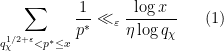
for any and , where the sum is over exceptional primes in the indicated range 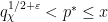; this bound is non-trivial for as large as . (See Section 1 of this blog post for some variants of this argument, which were inspired by work of Heath-Brown.) There is also a companion bound (somewhat weaker) that covers a range of a little bit below .

One of the early influential results in this area was the following result of Heath-Brown, which I previously blogged about here:

Theorem 1 (Hardy-Littlewood assuming Siegel zero) Let be a fixed natural number. Suppose one has a Siegel zero associated to some conductor . Then we have

for all , where is the von Mangoldt function and is the singular series

In particular, Heath-Brown showed that if there are infinitely many Siegel zeroes, then there are also infinitely many twin primes, with the correct asymptotic predicted by the Hardy-Littlewood prime tuple conjecture at infinitely many scales.

Very recently, Chinis established an analogous result for the Chowla conjecture (building upon earlier work of Germán and Katai):

Theorem 2 (Chowla assuming Siegel zero) Let be distinct fixed natural numbers. Suppose one has a Siegel zero associated to some conductor . Then one has

in the range , where is the Liouville function.

In our paper we unify these results and also improve the quantitative estimates and range of :

Theorem 3 (Hardy-Littlewood-Chowla assuming Siegel zero) Let be distinct fixed natural numbers with . Suppose one has a Siegel zero associated to some conductor . Then one has

for

for any fixed .

Our argument proceeds by a series of steps in which we replace and by more complicated looking, but also more tractable, approximations, until the correlation is one that can be computed in a tedious but straightforward fashion by known techniques. More precisely, the steps are as follows:

• (i) Replace the Liouville function with an approximant , which is a completely multiplicative function that agrees with at small primes and agrees with at large primes.
• (ii) Replace the von Mangoldt function with an approximant , which is the Dirichlet convolution multiplied by a Selberg sieve weight to essentially restrict that convolution to almost primes.
• (iii) Replace with a more complicated truncation which has the structure of a “Type I sum”, and which agrees with on numbers that have a “typical” factorization.
• (iv) Replace the approximant with a more complicated approximant which has the structure of a “Type I sum”.
• (v) Now that all terms in the correlation have been replaced with tractable Type I sums, use standard Euler product calculations and Fourier analysis, similar in spirit to the proof of the pseudorandomness of the Selberg sieve majorant for the primes in this paper of Ben Green and myself, to evaluate the correlation to high accuracy.

Steps (i), (ii) proceed mainly through estimates such as (1) and standard sieve theory bounds. Step (iii) is based primarily on estimates on the number of smooth numbers of a certain size.

The restriction in our main theorem is needed only to execute step (iv) of this step. Roughly speaking, the Siegel approximant to is a twisted, sieved version of the divisor function , and the types of correlation one is faced with at the start of step (iv) are a more complicated version of the divisor correlation sum

For this sum can be easily controlled by the Dirichlet hyperbola method. For one needs the fact that has a level of distribution greater than ; in fact Kloosterman sum bounds give a level of distribution of , a folklore fact that seems to have first been observed by Linnik and Selberg. We use a (notationally more complicated) version of this argument to treat the sums arising in (iv) for . Unfortunately for there are no known techniques to unconditionally obtain asymptotics, even for the model sum

although we do at least have fairly convincing conjectures as to what the asymptotics should be. Because of this, it seems unlikely that one will be able to relax the hypothesis in our main theorem at our current level of understanding of analytic number theory.

Step (v) is a tedious but straightforward sieve theoretic computation, similar in many ways to the correlation estimates of Goldston and Yildirim used in their work on small gaps between primes (as discussed for instance here), and then also used by Ben Green and myself to locate arithmetic progressions in primes.

Quantitative bounds for Gowers uniformity of the Mobius and von Mangoldt functions

Joni Teräväinen and myself have just uploaded to the arXiv our preprint “Quantitative bounds for Gowers uniformity of the Möbius and von Mangoldt functions“. This paper makes quantitative the Gowers uniformity estimates on the Möbius function and the von Mangoldt function .

To discuss the results we first discuss the situation of the Möbius function, which is technically simpler in some (though not all) ways. We assume familiarity with Gowers norms and standard notations around these norms, such as the averaging notation and the exponential notation . The prime number theorem in qualitative form asserts that

as . With Vinogradov-Korobov error term, the prime number theorem is strengthened to

we refer to such decay bounds (With type factors) as pseudopolynomial decay. Equivalently, we obtain pseudopolynomial decay of Gowers seminorm of :

As is well known, the Riemann hypothesis would be equivalent to an upgrade of this estimate to polynomial decay of the form

for any .

Once one restricts to arithmetic progressions, the situation gets worse: the Siegel-Walfisz theorem gives the bound

for any residue class and any , but with the catch that the implied constant is ineffective in . This ineffectivity cannot be removed without further progress on the notorious Siegel zero problem.

In 1937, Davenport was able to show the discorrelation estimate

for any uniformly in , which leads (by standard Fourier arguments) to the Fourier uniformity estimate

Again, the implied constant is ineffective. If one insists on effective constants, the best bound currently available is

for some small effective constant .

For the situation with the norm the previously known results were much weaker. Ben Green and I showed that

uniformly for any , any degree two (filtered) nilmanifold , any polynomial sequence , and any Lipschitz function ; again, the implied constants are ineffective. On the other hand, in a separate paper of Ben Green and myself, we established the following inverse theorem: if for instance we knew that

for some , then there exists a degree two nilmanifold of dimension , complexity , a polynomial sequence , and Lipschitz function of Lipschitz constant such that

Putting the two assertions together and comparing all the dependencies on parameters, one can establish the qualitative decay bound

However the decay rate produced by this argument is completely ineffective: obtaining a bound on when this quantity dips below a given threshold depends on the implied constant in (3) for some whose dimension depends on , and the dependence on obtained in this fashion is ineffective in the face of a Siegel zero.

For higher norms , the situation is even worse, because the quantitative inverse theory for these norms is poorer, and indeed it was only with the recent work of Manners that any such bound is available at all (at least for ). Basically, Manners establishes if

then there exists a degree nilmanifold of dimension , complexity , a polynomial sequence , and Lipschitz function of Lipschitz constant such that

(We allow all implied constants to depend on .) Meanwhile, the bound (3) was extended to arbitrary nilmanifolds by Ben and myself. Again, the two results when concatenated give the qualitative decay

but the decay rate is completely ineffective.

Our first result gives an effective decay bound:

Theorem 1 For any , we have for some . The implied constants are effective.

This is off by a logarithm from the best effective bound (2) in the case. In the case there is some hope to remove this logarithm based on the improved quantitative inverse theory currently available in this case, but there is a technical obstruction to doing so which we will discuss later in this post. For the above bound is the best one could hope to achieve purely using the quantitative inverse theory of Manners.

We have analogues of all the above results for the von Mangoldt function . Here a complication arises that does not have mean close to zero, and one has to subtract off some suitable approximant to before one would expect good Gowers norms bounds. For the prime number theorem one can just use the approximant , giving

but even for the prime number theorem in arithmetic progressions one needs a more accurate approximant. In our paper it is convenient to use the “Cramér approximant”

where

and is the quasipolynomial quantity

Then one can show from the Siegel-Walfisz theorem and standard bilinear sum methods that

and

for all and (with an ineffective dependence on ), again regaining effectivity if is replaced by a sufficiently small constant . All the previously stated discorrelation and Gowers uniformity results for then have analogues for , and our main result is similarly analogous:

Theorem 2 For any , we have for some . The implied constants are effective.

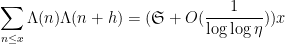
By standard methods, this result also gives quantitative asymptotics for counting solutions to various systems of linear equations in primes, with error terms that gain a factor of with respect to the main term.

We now discuss the methods of proof, focusing first on the case of the Möbius function. Suppose first that there is no “Siegel zero”, by which we mean a quadratic character of some conductor with a zero with for some small absolute constant . In this case the Siegel-Walfisz bound (1) improves to a quasipolynomial bound

To establish Theorem 1 in this case, it suffices by Manners’ inverse theorem to establish the polylogarithmic bound

for all degree nilmanifolds of dimension and complexity , all polynomial sequences , and all Lipschitz functions of norm . If the nilmanifold had bounded dimension, then one could repeat the arguments of Ben and myself more or less verbatim to establish this claim from (5), which relied on the quantitative equidistribution theory on nilmanifolds developed in a separate paper of Ben and myself. Unfortunately, in the latter paper the dependence of the quantitative bounds on the dimension was not explicitly given. In an appendix to the current paper, we go through that paper to account for this dependence, showing that all exponents depend at most doubly exponentially in the dimension , which is barely sufficient to handle the dimension of that arises here.

Now suppose we have a Siegel zero . In this case the bound (5) will not hold in general, and hence also (6) will not hold either. Here, the usual way out (while still maintaining effective estimates) is to approximate not by , but rather by a more complicated approximant that takes the Siegel zero into account, and in particular is such that one has the (effective) pseudopolynomial bound

for all residue classes . The Siegel approximant to is actually a little bit complicated, and to our knowledge the first appearance of this sort of approximant only appears as late as this 2010 paper of Germán and Katai. Our version of this approximant is defined as the multiplicative function such that

when , and

when is coprime to all primes , and is a normalising constant given by the formula

(this constant ends up being of size and plays only a minor role in the analysis). This is a rather complicated formula, but it seems to be virtually the only choice of approximant that allows for bounds such as (7) to hold. (This is the one aspect of the problem where the von Mangoldt theory is simpler than the Möbius theory, as in the former one only needs to work with very rough numbers for which one does not need to make any special accommodations for the behavior at small primes when introducing the Siegel correction term.) With this starting point it is then possible to repeat the analysis of my previous papers with Ben and obtain the pseudopolynomial discorrelation bound

for as before, which when combined with Manners’ inverse theorem gives the doubly logarithmic bound

Meanwhile, a direct sieve-theoretic computation ends up giving the singly logarithmic bound

(indeed, there is a good chance that one could improve the bounds even further, though it is not helpful for this current argument to do so). Theorem 1 then follows from the triangle inequality for the Gowers norm. It is interesting that the Siegel approximant seems to play a rather essential component in the proof, even if it is absent in the final statement. We note that this approximant seems to be a useful tool to explore the “illusory world” of the Siegel zero further; see for instance the recent paper of Chinis for some work in this direction.

For the analogous problem with the von Mangoldt function (assuming a Siegel zero for sake of discussion), the approximant is simpler; we ended up using

which allows one to state the standard prime number theorem in arithmetic progressions with classical error term and Siegel zero term compactly as

Routine modifications of previous arguments also give

and

The one tricky new step is getting from the discorrelation estimate (8) to the Gowers uniformity estimate

One cannot directly apply Manners’ inverse theorem here because and are unbounded. There is a standard tool for getting around this issue, now known as the dense model theorem, which is the standard engine powering the transference principle from theorems about bounded functions to theorems about certain types of unbounded functions. However the quantitative versions of the dense model theorem in the literature are expensive and would basically weaken the doubly logarithmic gain here to a triply logarithmic one. Instead, we bypass the dense model theorem and directly transfer the inverse theorem for bounded functions to an inverse theorem for unbounded functions by using the densification approach to transference introduced by Conlon, Fox, and Zhao. This technique turns out to be quantitatively quite efficient (the dependencies of the main parameters in the transference are polynomial in nature), and also has the technical advantage of avoiding the somewhat tricky “correlation condition” present in early transference results which are also not beneficial for quantitative bounds.

In principle, the above results can be improved for due to the stronger quantitative inverse theorems in the setting. However, there is a bottleneck that prevents us from achieving this, namely that the equidistribution theory of two-step nilmanifolds has exponents which are exponential in the dimension rather than polynomial in the dimension, and as a consequence we were unable to improve upon the doubly logarithmic results. Specifically, if one is given a sequence of bracket quadratics such as that fails to be -equidistributed, one would need to establish a nontrivial linear relationship modulo 1 between the (up to errors of ), where the coefficients are of size ; current methods only give coefficient bounds of the form . An old result of Schmidt demonstrates proof of concept that these sorts of polynomial dependencies on exponents is possible in principle, but actually implementing Schmidt’s methods here seems to be a quite non-trivial task. There is also another possible route to removing a logarithm, which is to strengthen the inverse theorem to make the dimension of the nilmanifold logarithmic in the uniformity parameter rather than polynomial. Again, the Freiman-Bilu theorem (see for instance this paper of Ben and myself) demonstrates proof of concept that such an improvement in dimension is possible, but some work would be needed to implement it.

Singmaster’s conjecture in the interior of Pascal’s triangle

Kaisa Matomäki, Maksym Radziwill, Xuancheng Shao, Joni Teräväinen, and myself have just uploaded to the arXiv our preprint “Singmaster’s conjecture in the interior of Pascal’s triangle“. This paper leverages the theory of exponential sums over primes to make progress on a well known conjecture of Singmaster which asserts that any natural number larger than appears at most a bounded number of times in Pascal’s triangle. That is to say, for any integer , there are at most solutions to the equation

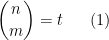
with . Currently, the largest number of solutions that is known to be attainable is eight, with equal to

Because of the symmetry of Pascal’s triangle it is natural to restrict attention to the left half of the triangle.

Our main result settles this conjecture in the “interior” region of the triangle:

Theorem 1 (Singmaster’s conjecture in the interior of the triangle) If and is sufficiently large depending on , there are at most two solutions to (1) in the region

and hence at most four in the region

Also, there is at most one solution in the region

To verify Singmaster’s conjecture in full, it thus suffices in view of this result to verify the conjecture in the boundary region

(or equivalently ); we have deleted the case as it of course automatically supplies exactly one solution to (1). It is in fact possible that for sufficiently large there are no further collisions for in the region (3), in which case there would never be more than eight solutions to (1) for sufficiently large . This is latter claim known for bounded values of by Beukers, Shorey, and Tildeman, with the main tool used being Siegel’s theorem on integral points.

The upper bound of two here for the number of solutions in the region (2) is best possible, due to the infinite family of solutions to the equation

coming from , and is the Fibonacci number.

The appearance of the quantity in Theorem 1 may be familiar to readers that are acquainted with Vinogradov’s bounds on exponential sums, which ends up being the main new ingredient in our arguments. In principle this threshold could be lowered if we had stronger bounds on exponential sums.

To try to control solutions to (1) we use a combination of “Archimedean” and “non-Archimedean” approaches. In the “Archimedean” approach (following earlier work of Kane on this problem) we view primarily as real numbers rather than integers, and express (1) in terms of the Gamma function as

One can use this equation to solve for in terms of as

for a certain real analytic function whose asymptotics are easily computable (for instance one has the asymptotic ). One can then view the problem as one of trying to control the number of lattice points on the graph . Here we can take advantage of the fact that in the regime (which corresponds to working in the left half of Pascal’s triangle), the function can be shown to be convex, but not too convex, in the sense that one has both upper and lower bounds on the second derivative of (in fact one can show that ). This can be used to preclude the possibility of having a cluster of three or more nearby lattice points on the graph , basically because the area subtended by the triangle connecting three of these points would lie between and , contradicting Pick’s theorem. Developing these ideas, we were able to show

Proposition 2 Let , and suppose is sufficiently large depending on . If is a solution to (1) in the left half of Pascal’s triangle, then there is at most one other solution to this equation in the left half with

Again, the example of (4) shows that a cluster of two solutions is certainly possible; the convexity argument only kicks in once one has a cluster of three or more solutions.

To finish the proof of Theorem 1, one has to show that any two solutions to (1) in the region of interest must be close enough for the above proposition to apply. Here we switch to the “non-Archimedean” approach, in which we look at the -adic valuations of the binomial coefficients, defined as the number of times a prime divides . From the fundamental theorem of arithmetic, a collision

between binomial coefficients occurs if and only if one has agreement of valuations

From the Legendre formula

we can rewrite this latter identity (5) as

where denotes the fractional part of . (These sums are not truly infinite, because the summands vanish once is larger than .)

A key idea in our approach is to view this condition (6) statistically, for instance by viewing as a prime drawn randomly from an interval such as for some suitably chosen scale parameter , so that the two sides of (6) now become random variables. It then becomes advantageous to compare correlations between these two random variables and some additional test random variable. For instance, if and are far apart from each other, then one would expect the left-hand side of (6) to have a higher correlation with the fractional part , since this term shows up in the summation on the left-hand side but not the right. Similarly if and are far apart from each other (although there are some annoying cases one has to treat separately when there is some “unexpected commensurability”, for instance if is a rational multiple of where the rational has bounded numerator and denominator). In order to execute this strategy, it turns out (after some standard Fourier expansion) that one needs to get good control on exponential sums such as

for various choices of parameters , where . Fortunately, the methods of Vinogradov (which more generally can handle sums such as and for various analytic functions ) can give useful bounds on such sums as long as and are not too large compared to ; more specifically, Vinogradov’s estimates are non-trivial in the regime , and this ultimately leads to a distance bound

between any colliding pair in the left half of Pascal’s triangle, as well as the variant bound

under the additional assumption

Comparing these bounds with Proposition 2 and using some basic estimates about the function , we can conclude Theorem 1.

A modification of the arguments also gives similar results for the equation

where is the falling factorial:

Theorem 3 If and is sufficiently large depending on , there are at most two solutions to (7) in the region

Again the upper bound of two is best possible, thanks to identities such as