
You are currently browsing the tag archive for the ‘additive combinatorics’ tag.
Tim Gowers, Ben Green, Freddie Manners, and I have just uploaded to the arXiv our paper “Marton’s conjecture in abelian groups with bounded torsion“. This paper fully resolves a conjecture of Katalin Marton (the bounded torsion case of the Polynomial Freiman–Ruzsa conjecture (first proposed by Katalin Marton):
Theorem 1 (Marton’s conjecture) Let
be an abelian
-torsion group (thus,
for all
), and let
be such that
. Then
can be covered by at most
translates of a subgroup
of
of cardinality at most
. Moreover,
for some
.
We had previously established the 


Our proof techniques are a modification of those in our previous paper, and in particular continue to be based on the theory of Shannon entropy. For inductive purposes, it turns out to be convenient to work with the following version of the conjecture (which, up to
Theorem 2 (Marton’s conjecture, entropy form) Let
be independent finitely supported random variables on
where
denotes Shannon entropy. Then there is a uniform random variable
on a subgroup
where
denotes the entropic Ruzsa distance (see previous blog post for a definition); furthermore, if all the
take values in some symmetric set
, then
for some
.
![\displaystyle {\bf H}[X_1+\dots+X_m] - \frac{1}{m} \sum_{i=1}^m {\bf H}[X_i] \leq \log K,](https://s0.wp.com/latex.php?latex=%5Cdisplaystyle+%7B%5Cbf+H%7D%5BX_1%2B%5Cdots%2BX_m%5D+-+%5Cfrac%7B1%7D%7Bm%7D+%5Csum_%7Bi%3D1%7D%5Em+%7B%5Cbf+H%7D%5BX_i%5D+%5Cleq+%5Clog+K%2C&bg=ffffff&fg=000000&s=0&c=20201002)
![\displaystyle \frac{1}{m} \sum_{i=1}^m d[X_i; U_H] \ll m^3 \log K,](https://s0.wp.com/latex.php?latex=%5Cdisplaystyle+%5Cfrac%7B1%7D%7Bm%7D+%5Csum_%7Bi%3D1%7D%5Em+d%5BX_i%3B+U_H%5D+%5Cll+m%5E3+%5Clog+K%2C&bg=ffffff&fg=000000&s=0&c=20201002)
As a first approximation, one should think of all the
The strategy, as with the previous paper, is to attempt an entropy decrement argument: to try to locate modifications 
![\displaystyle {\bf H}[X_1+\dots+X_m] - \frac{1}{m} \sum_{i=1}^m {\bf H}[X_i]](https://s0.wp.com/latex.php?latex=%5Cdisplaystyle+%7B%5Cbf+H%7D%5BX_1%2B%5Cdots%2BX_m%5D+-+%5Cfrac%7B1%7D%7Bm%7D+%5Csum_%7Bi%3D1%7D%5Em+%7B%5Cbf+H%7D%5BX_i%5D+&bg=ffffff&fg=000000&s=0&c=20201002)
which turns out to be a convenient metric for progress (for instance, this quantity is non-negative, and vanishes if and only if the 
As before, we search for such improved random variables 


Up until now, the argument does not use the 

In the endgame, the any pair of these three random variables are close to independent (after conditioning on the total sum 
Besides the polynomial Bogolyubov conjecture mentioned above (which we do not know how to address by entropy methods), the other natural question is to try to develop a characteristic zero version of this theory in order to establish the polynomial Freiman–Ruzsa conjecture over torsion-free groups, which in our language asserts (roughly speaking) that random variables of small entropic doubling are close (in Ruzsa distance) to a discrete Gaussian random variable, with good bounds. The above machinery is consistent with this conjecture, in that it produces lots of independent variables related to the original variable, various linear combinations of which obey the same sort of entropy estimates that gaussian random variables would exhibit, but what we are missing is a way to get back from these entropy estimates to an assertion that the random variables really are close to Gaussian in some sense. In continuous settings, Gaussians are known to extremize the entropy for a given variance, and of course we have the central limit theorem that shows that averages of random variables typically converge to a Gaussian, but it is not clear how to adapt these phenomena to the discrete Gaussian setting (without the circular reasoning of assuming the polynoimal Freiman–Ruzsa conjecture to begin with).
Tim Gowers, Ben Green, Freddie Manners, and I have just uploaded to the arXiv our paper “On a conjecture of Marton“. This paper establishes a version of the notorious Polynomial Freiman–Ruzsa conjecture (first proposed by Katalin Marton):
Theorem 1 (Polynomial Freiman–Ruzsa conjecture) Letbe such that
translates of a subspace
of cardinality at most
The previous best known result towards this conjecture was by Konyagin (as communicated in this paper of Sanders), who obtained a similar result but with 


The exponent 
In this paper we will focus exclusively on the characteristic
Much of the prior progress on this sort of result has proceeded via Fourier analysis. Perhaps surprisingly, our approach uses no Fourier analysis whatsoever, being conducted instead entirely in “physical space”. Broadly speaking, it follows a natural strategy, which is to induct on the doubling constant 


 to means that the various Ruzsa distances that need to be summed are controlled by a convergent geometric series).
There are a number of possible ways to try to “improve” a set
- (i) Replacing
) of a large subspace
- (ii) Replacing
for a “typical”
. For instance, if
Unfortunately, there are sets 

This begins to suggest a potential strategy: show that at least one of the operations (i) or (ii) will improve the doubling constant, or at least not worsen it too much; and in the latter case, perform some more complicated operation to locate the desired doubling constant improvement.
A sign that this strategy might have a chance of working is provided by the following heuristic argument. If 


Unfortunately, this argument does not seem to be easily made rigorous using the traditional doubling constant; even the significantly weaker statement that 


 is defined as


Applying this inequality with 


 is determined by
  once one fixes
  )
) 
 , then at least one of
  or
or  will be less than or equal to
  . This is the entropy analogue of at least one of (i) or (ii) improving, or at least not degrading the doubling constant, although there are some minor technicalities involving how one deals with the conditioning to in the second term that we will gloss over here (one can pigeonhole the instances of to different events
  ,
,  , and “depolarise” the induction hypothesis to deal with distances
  between pairs of random variables that do not necessarily have the same distribution). Furthermore, we can even calculate the defect in the above inequality: a careful inspection of the above argument eventually reveals that

 . This leads (modulo some technicalities) to the following interesting conclusion: if neither (i) nor (ii) leads to an improvement in the entropic doubling constant, then and
  are conditionally independent relative to
  . This situation (or an approximation to this situation) is what we refer to in the paper as the “endgame”.
A version of this endgame conclusion is in fact valid in any characteristic. But in characteristic
 , and using symmetry we now conclude that if we are in the endgame exactly (so that the mutual information is zero), then the independent sum of two copies of
  has exactly the same distribution; in particular, the entropic doubling constant here is zero, which is certainly a reduction in the doubling constant.
To deal with the situation where the conditional mutual information is small but not completely zero, we have to use an entropic version of the Balog-Szemeredi-Gowers lemma, but fortunately this was already worked out in an old paper of mine (although in order to optimise the final constant, we ended up using a slight variant of that lemma).
I am planning to formalize this paper in the Lean4 language. Further discussion of this project will take place on this Zulip stream, and the project itself will be held at this Github repository.
Asgar Jamneshan and myself have just uploaded to the arXiv our preprint “The inverse theorem for the 
 , where
  is the multiplicative derivative. Our main result is as follows:
Theorem 1 (Inverse theorem for) Let
be a
for some
. Then:
- (i) (Correlation with locally quadratic phase) There exists a regular Bohr set
with
and
, a locally quadratic function
, and a function
such that
- (ii) (Correlation with nilsequence) There exists an explicit degree two filtered nilmanifold
of dimension
, a polynomial map
, and a Lipschitz function
of constant
such that


Such a theorem was proven by Ben Green and myself in the case when 


 denotes various -bounded functions whose exact values are not too important, and
  is a symmetric locally bilinear form. The idea is then to “integrate” this form by expressing it in the form
 ; this then allows us to write the above correlation as
  functions suitably), and one can now conclude part (i) of the above theorem using some linear Fourier analysis. Part (ii) follows by encoding locally quadratic phase functions as nilsequences; for this we adapt an algebraic construction of Manners.
So the key step is to obtain a representation of the form (1), possibly after shrinking the Bohr set 
- When
one can establish (1) with
. (This is similar to how in single variable calculus the function
is a function whose second derivative is equal to
- When
for some
for somewith
. The diagonal terms
cause a problem, but by subtracting off the rank one form
one can write
on the orthogonal complement offor some coefficients
which now vanish on the diagonal:
. One can now obtain (1) on this complement by taking


In our paper we can now treat the case of arbitrary finite abelian groups
- (i) Using some geometry of numbers, we can lift the group
with a projection map
, and find a globally bilinear map
on the latter group, such that one has a representation
of the locally bilinear formby the globally bilinear form
when
are close enough to the origin.
- (ii) Using an explicit construction, one can show that every globally bilinear map
.

To illustrate (i), consider the Bohr set 


 ) and introduces the globally bilinear form by the formula
 lie in the interval
  . A similar construction works for higher rank Bohr sets.
To illustrate (ii), the key case turns out to be when 
 . One can then check by direct construction that (1) will be obeyed with
 is even or odd. A variant of this construction also works for
  , and the general case follows from a short calculation verifying that the claim (ii) for any two groups
  implies the corresponding claim (ii) for the product
  .
.
This concludes the Fourier-analytic proof of Theorem 1. In this paper we also give an ergodic theory proof of (a qualitative version of) Theorem 1(ii), using a correspondence principle argument adapted from this previous paper of Ziegler, and myself. Basically, the idea is to randomly generate a dynamical system on the group 

 where the size of goes to infinity), and that the dynamical Host-Kra-Gowers seminorms of that system coincide with the combinatorial Gowers norms of the original functions. One is then well placed to apply an inverse theorem for the third Host-Kra-Gowers seminorm
  for
for  -actions, which was accomplished in the companion paper to this one. After doing so, one almost gets the desired conclusion of Theorem 1(ii), except that after undoing the application of the Furstenberg correspondence principle, the map is merely an almost polynomial rather than a polynomial, which roughly speaking means that instead of certain derivatives of
  vanishing, they instead are merely very small outside of a small exceptional set. To conclude we need to invoke a “stability of polynomials” result, which at this level of generality was first established by Candela and Szegedy (though we also provide an independent proof here in an appendix), which roughly speaking asserts that every approximate polynomial is close in measure to an actual polynomial. (This general strategy is also employed in the Candela-Szegedy paper, though in the absence of the ergodic inverse theorem input that we rely upon here, the conclusion is weaker in that the filtered nilmanifold is replaced with a general space known as a “CFR nilspace”.)
This transference principle approach seems to work well for the higher step cases (for instance, the stability of polynomials result is known in arbitrary degree); the main difficulty is to establish a suitable higher step inverse theorem in the ergodic theory setting, which we hope to do in future research.
Laura Cladek and I have just uploaded to the arXiv our paper “Additive energy of regular measures in one and higher dimensions, and the fractal uncertainty principle“. This paper concerns a continuous version of the notion of additive energy. Given a finite measure 


 and some constants
  , as well as the matching lower bound
 whenever
  . One should think of as a
  -dimensional fractal set, and as some vaguely self-similar measure on this set.
Note that once one fixes 


Theorem 1 Ifis not an integer, and
are as above, then
for some
depending only on
.
Informally, this asserts that Ahlfors-David regular fractal sets of non-integer dimension cannot behave as if they are approximately closed under addition. In fact the gain 
 and .) Such a result was previously obtained (with more explicit values of the
  implied constants) in the one-dimensional case
  by Dyatlov and Zahl; but in higher dimensions there does not appear to have been any results for this general class of sets and measures . In the paper of Dyatlov and Zahl it is noted that some dependence on is necessary; in particular, cannot be much better than
  . This reflects the fact that there are fractal sets that do behave reasonably well with respect to addition (basically because they are built out of long arithmetic progressions at many scales); however, such sets are not very Ahlfors-David regular. Among other things, this result readily implies a dimension expansion result
 , including the sum map
  and (in one dimension) the product map
  , where the non-degeneracy condition required is that the gradients
  are invertible for every . We refer to the paper for the formal statement.
Our higher-dimensional argument shares many features in common with that of Dyatlov and Zahl, notably a reliance on the modern tools of additive combinatorics (and specifically the Bogulybov-Ruzsa lemma of Sanders). However, in one dimension we were also able to find a completely elementary argument, avoiding any particularly advanced additive combinatorics and instead primarily exploiting the order-theoretic properties of the real line, that gave a superior value of
One of the main reasons for obtaining such improved energy bounds is that they imply a fractal uncertainty principle in some regimes. We focus attention on the model case of obtaining such an uncertainty principle for the semiclassical Fourier transform
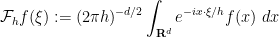
 is a small parameter. If
  are as above, and
  denotes the
  -neighbourhood of , then from the Hausdorff-Young inequality one obtains the trivial bound
 , but for simplicity we focus on the uncertainty principle for a single set .) The fractal uncertainty principle, when it applies, asserts that one can improve this to
  ; informally, this asserts that a function and its Fourier transform cannot simultaneously be concentrated in the set when
  , and that a function cannot be concentrated on and have its Fourier transform be of maximum size on when
  . A modification of the disk example mentioned previously shows that such a fractal uncertainty principle cannot hold if is an integer. However, in one dimension, the fractal uncertainty principle is known to hold for all
  . The above-mentioned results of Dyatlov and Zahl were able to establish this for close to
  , and the remaining cases
  and
and  were later established by Bourgain-Dyatlov and Dyatlov-Jin respectively. Such uncertainty principles have applications to hyperbolic dynamics, in particular in establishing spectral gaps for certain Selberg zeta functions.
It remains a largely open problem to establish a fractal uncertainty principle in higher dimensions. Our results allow one to establish such a principle when the dimension 
We now sketch how our main theorem is proved. In both one dimension and higher dimensions, the main point is to get a preliminary improvement 


It remains to obtain the preliminary improvement. In one dimension this is done by identifying some “left edges” of the set ![{[x, x+K^{-n}]}](https://s0.wp.com/latex.php?latex=%7B%5Bx%2C+x%2BK%5E%7B-n%7D%5D%7D&bg=ffffff&fg=000000&s=0&c=20201002)
![{[x-K^{-n+1},x]}](https://s0.wp.com/latex.php?latex=%7B%5Bx-K%5E%7B-n%2B1%7D%2Cx%5D%7D&bg=ffffff&fg=000000&s=0&c=20201002)


![{[x,x+K^{-n}] \times [y,y+K^{-n}]}](https://s0.wp.com/latex.php?latex=%7B%5Bx%2Cx%2BK%5E%7B-n%7D%5D+%5Ctimes+%5By%2Cy%2BK%5E%7B-n%7D%5D%7D&bg=ffffff&fg=000000&s=0&c=20201002)


We were not able to make this argument work in higher dimension (though perhaps the cases 


Let 


for all 

for all additive quadruples 


Now suppose that

for all 

for all additive quadruples
“Trivial” examples of quasimorphisms include the sum of a homomorphism and a bounded function. Are there others? In some cases, the answer is no. For instance, suppose we have a quasimorphism 


In general, one can phrase this problem in the language of group cohomology (discussed in this previous post). Call a map 

for all 


Such functions are called 
If a 

In additive combinatorics, one is often working with functions which only have additive structure a fraction of the time, thus for instance (1) or (3) might only hold “

Theorem 1 Let
, let
, and let
be a function such that
for
additive quadruples
. Then there exists a subset
, a subset
, and a function
such that
for all
(thus, the derivative
takes values in
on
), and such that for each
, one has
for
values of
.


Presumably the constants 


Proof: By hypothesis, there are 


Thus, there is a set 


for
Consider the bipartite graph whose vertex sets are two copies of 


and 


Also observe that

Thus, if 


for 

By the pigeonhole principle, this implies that for any fixed 


whenever

This implies that there exists a subset 

for all 

 are such that
By construction of 


and

for 

and hence by (8)

where 
we see that there are only 


whenever (10) holds.
For any 


Then from (11) we have (4). For 

A sequence 

for some real numbers 


with 

These sequences arise in various “complexity one” problems in arithmetic combinatorics and ergodic theory. For instance, if 


can be shown to be an almost periodic sequence, plus an error term 

This can be established in a number of ways, for instance by writing 


In the last two decades or so, it has become clear that there are natural higher order versions of these concepts, in which linear polynomials such as 

For technical reasons (having to do with the non-trivial topological structure on nilmanifolds), it will be convenient to work with vector-valued sequences, that take values in a finite-dimensional complex vector space 


This product is associative and bilinear, and also commutative up to permutation of the indices. It also interacts well with the Hermitian norm

since we have 
The traditional definition of a basic nilsequence (as defined for instance by Bergelson, Host, and Kra) is as follows:
Definition 1 (Basic nilsequence, first definition) A nilmanifold of step at most
, where
-fold commutators vanish) and
is a discrete cocompact lattice in
, where
,
, and
is a continuous function.
For instance, it is not difficult using this definition to show that a sequence is a basic nilsequence of degree at most 
Nowadays, and particularly when one needs to understand the “single-scale” equidistribution properties of nilsequences, it is more convenient (as is for instance done in this ICM paper of Green) to use an alternate definition of a nilsequence as follows.
Definition 2 Let
. A filtered group of degree at most
of subgroups
with
and
for
. A polynomial sequence
into a filtered group is a function such that
for all
and
, where
is the difference operator. A filtered nilmanifold of degree at most
is a quotient
are connected, simply connected nilpotent filtered Lie group, and
is a discrete cocompact subgroup of
, where
is a continuous function which is
for all
.
One can easily identify a 

It is easy to see that any sequence that is a basic nilsequence of degree at most 

where 


The other key example is a sequence of the form
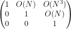
where 


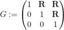
with the lower central series filtration 
![{G_2= [G,G] = \begin{pmatrix} 1 &0 & {\bf R} \\ 0 & 1 & 0 \\ 0 & 0 & 1 \end{pmatrix}}](https://s0.wp.com/latex.php?latex=%7BG_2%3D+%5BG%2CG%5D+%3D+%5Cbegin%7Bpmatrix%7D+1+%260+%26+%7B%5Cbf+R%7D+%5C%5C+0+%26+1+%26+0+%5C%5C+0+%26+0+%26+1+%5Cend%7Bpmatrix%7D%7D&bg=ffffff&fg=000000&s=0&c=20201002)


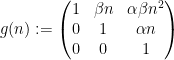
and 

one easily verifies that this function is indeed 


will be a basic nilsequence if 
A nilsequence of degree at most 


is equal to a nilsequence of degree at most 

It is easy to see that a sequence 

Now we turn to the notion of a nilcharacter, as defined in this paper of Ben Green, Tamar Ziegler, and myself:
Definition 3 (Nilcharacters) Let
. A sub-nilcharacter of degree
of degree at most
for all
, where
is a continuous homomorphism
. (Note from (1) and
must map
to
.) If in addition one has
for all
a nilcharacter of degree

In the degree one case 


where 

for all 


We claim that every degree 


and then

becomes a degree 
As we shall show below, nilsequences can be approximated uniformly by linear combinations of nilcharacters, in much the same way that quasiperiodic or almost periodic sequences can be approximated uniformly by linear combinations of linear phases. In particular, nilcharacters can be used as “obstructions to uniformity” in the sense of the inverse theory of the Gowers uniformity norms.
The space of degree
Definition 4 Let
,
are equivalent if
is equal (as a sequence) to a basic nilsequence of degree at most
of such a nilcharacter will be called the symbol of that nilcharacter (in analogy to the symbol of a differential or pseudodifferential operator), and the collection of such symbols will be denoted
.
As we shall see below the fold, 


Van Vu and I just posted to the arXiv our paper “sum-free sets in groups” (submitted to Discrete Analysis), as well as a companion survey article (submitted to J. Comb.). Given a subset 


If
 natural numbers. Then
  .
.Proof: We use an argument of Ruzsa, which is based in turn on an older argument of Choi. Let 


In particular, we have 

a result of Shao (building upon earlier work of Sudakov, Szemeredi, and Vu and of Dousse). In the opposite direction, a construction of Ruzsa gives examples of large sets 
Using the standard tool of Freiman homomorphisms, the above results for the integers extend to other torsion-free abelian groups 


Theorem 2 For every
there exists
such that if
, then there exist
There are two main tools used to prove this result. One is an “arithmetic removal lemma” proven by Král, Serra, and Vena. Note that the condition 


The second tool is the following structure theorem, which is the main result of our paper, and goes a fair ways towards classifying sets
Theorem 3 Let
with
such that
and
. Furthermore, if
, then the exceptional set
is empty.
Roughly speaking, this theorem shows that the example of the union of
This theorem has the flavour of other inverse theorems in additive combinatorics, such as Freiman’s theorem, and indeed one can use Freiman’s theorem (and related tools, such as the Balog-Szemeredi theorem) to easily get a weaker version of this theorem. Indeed, if there are no sum-free subsets of 


At this point it is tempting to simply remove 


I’ve just uploaded to the arXiv my paper “Inverse theorems for sets and measures of polynomial growth“. This paper was motivated by two related questions. The first question was to obtain a qualitatively precise description of the sets of polynomial growth that arise in Gromov’s theorem, in much the same way that Freiman’s theorem (and its generalisations) provide a qualitatively precise description of sets of small doubling. The other question was to obtain a non-abelian analogue of inverse Littlewood-Offord theory.
Let me discuss the former question first. Gromov’s theorem tells us that if a finite subset 


In this paper we are able to refine this analysis a bit further; under the same hypotheses, we can show an estimate of the form

for all 


One could ask whether the function 


To prove this proposition, it turns out (after using a somewhat difficult inverse theorem proven previously by Breuillard, Green, and myself) that one has to analyse the volume growth 


The arguments also give a precise description of the location of a set 


The main tool used to prove these results is the structure theorem for approximate groups established by Breuillard, Green, and myself, which roughly speaking asserts that approximate groups are always commensurate with coset nilprogressions. A key additional trick is a pigeonholing argument of Sanders, which in this context is the assertion that if 


Similar arguments apply when discussing iterated convolutions 


A special case of this theory occurs when 


Suppose that 
![{K := [B:A]}](https://s0.wp.com/latex.php?latex=%7BK+%3A%3D+%5BB%3AA%5D%7D&bg=ffffff&fg=000000&s=0&c=20201002)


Even if 

![\displaystyle [A : A \cap B], [B : A \cap B] \leq K.](https://s0.wp.com/latex.php?latex=%5Cdisplaystyle++%5BA+%3A+A+%5Ccap+B%5D%2C+%5BB+%3A+A+%5Ccap+B%5D+%5Cleq+K.&bg=ffffff&fg=000000&s=0&c=20201002)
Proposition 1 Let
. Then for every
, the groups
are
![\displaystyle [A : A \cap A^s ] = [A^s : A \cap A^s ] \leq K.](https://s0.wp.com/latex.php?latex=%5Cdisplaystyle++%5BA+%3A+A+%5Ccap+A%5Es+%5D+%3D+%5BA%5Es+%3A+A+%5Ccap+A%5Es+%5D+%5Cleq+K.&bg=ffffff&fg=000000&s=0&c=20201002)
Proof: One can partition 


![{[B: A \cap A^s] \leq K^2}](https://s0.wp.com/latex.php?latex=%7B%5BB%3A+A+%5Ccap+A%5Es%5D+%5Cleq+K%5E2%7D&bg=ffffff&fg=000000&s=0&c=20201002)
![\displaystyle [B: A \cap A^s] = [B:A] [A: A \cap A^s] = [B:A^s] [A^s: A \cap A^s]](https://s0.wp.com/latex.php?latex=%5Cdisplaystyle+%5BB%3A+A+%5Ccap+A%5Es%5D+%3D+%5BB%3AA%5D+%5BA%3A+A+%5Ccap+A%5Es%5D+%3D+%5BB%3AA%5Es%5D+%5BA%5Es%3A+A+%5Ccap+A%5Es%5D+&bg=ffffff&fg=000000&s=0&c=20201002)
and ![{[B:A] = [B:A^s]=K}](https://s0.wp.com/latex.php?latex=%7B%5BB%3AA%5D+%3D+%5BB%3AA%5Es%5D%3DK%7D&bg=ffffff&fg=000000&s=0&c=20201002)
One can replace the inclusion
Corollary 2 Let
be
Proof: Applying the previous proposition with 

It turns out that a similar phenomenon holds for the more general concept of an approximate group, and gives a “classification” of all the approximate groups 
note that this is consistent with the previous notion of commensurability for genuine groups.
Theorem 3 Let
be real numbers. Let
-approximate group, and let
- (i) If
-approximate group with
, then one has
for some set
. Furthermore, for each
-commensurate.
- (ii) Conversely, if
, and
-approximate group.
Informally, the assertion that 


To prove the theorem, we recall some standard lemmas from arithmetic combinatorics, which are the foundation stones of the “Ruzsa calculus” that we will use to establish our results:
Lemma 4 (Ruzsa covering lemma) If
for some set
.
Proof: We take 

Lemma 5 (Ruzsa triangle inequality) If
are finite non-empty subsets of

Proof: If 


Now we can prove (i). By the Ruzsa covering lemma,

left-translates of 


and hence for any


By the Ruzsa covering lemma again, this implies that 

Since

and

the claim follows.
Now we prove (ii). Clearly

Now we control the size of 

From the Ruzsa triangle inequality and symmetry we have


and thus

By the Ruzsa covering lemma, this implies that 

We now establish some auxiliary propositions about commensurability of approximate groups. The first claim is that commensurability is approximately transitive:
Proposition 6 Let
-commensurate, and
-commensurate, then
-commensurate.
Proof: From two applications of the Ruzsa triangle inequality we have


By the Ruzsa covering lemma, we may thus cover 


and so by arguing as in the proof of part (i) of the theorem we have

and similarly

and the claim follows.
The next proposition asserts that the union and (modified) intersection of two commensurate approximate groups is again an approximate group:
Proposition 7 Let
is a
-approximate subgroup, and
is a
-approximate subgroup.
Using this proposition, one may obtain a variant of the previous theorem where the containment
Proof: We begin with 


and hence by the Ruzsa covering lemma, 


Now we consider

Now observe that

and so by the Ruzsa covering lemma, 

In graph theory, the recently developed theory of graph limits has proven to be a useful tool for analysing large dense graphs, being a convenient reformulation of the Szemerédi regularity lemma. Roughly speaking, the theory asserts that given any sequence 

![{p\colon [0,1] \times [0,1] \rightarrow [0,1]}](https://s0.wp.com/latex.php?latex=%7Bp%5Ccolon+%5B0%2C1%5D+%5Ctimes+%5B0%2C1%5D+%5Crightarrow+%5B0%2C1%5D%7D&bg=ffffff&fg=000000&s=0&c=20201002)


converge to the integral
the triangle density

converges to the integral

the four-cycle density

converges to the integral

and so forth. One can use graph limits to prove many results in graph theory that were traditionally proven using the regularity lemma, such as the triangle removal lemma, and can also reduce many asymptotic graph theory problems to continuous problems involving multilinear integrals (although the latter problems are not necessarily easy to solve!). See this text of Lovasz for a detailed study of graph limits and their applications.
One can also express graph limits (and more generally hypergraph limits) in the language of nonstandard analysis (or of ultraproducts); see for instance this paper of Elek and Szegedy, Section 6 of this previous blog post, or this paper of Towsner. (In this post we assume some familiarity with nonstandard analysis, as reviewed for instance in the previous blog post.) Here, one starts as before with a sequence 


where the “graphon” 


![{p\colon V_\alpha \times V_\alpha \rightarrow [0,1]}](https://s0.wp.com/latex.php?latex=%7Bp%5Ccolon+V_%5Calpha+%5Ctimes+V_%5Calpha+%5Crightarrow+%5B0%2C1%5D%7D&bg=ffffff&fg=000000&s=0&c=20201002)


(or equivalently, the limit of the 
where 


(or equivalently, the limit along 

and so forth. Note that with this construction, the graphon ![{[0,1]}](https://s0.wp.com/latex.php?latex=%7B%5B0%2C1%5D%7D&bg=ffffff&fg=000000&s=0&c=20201002)
Additive combinatorics, which studies things like the additive structure of finite subsets
It seems that to allow for the most flexible and powerful manifestation of this theory, it is convenient to use the nonstandard formulation (among other things, it allows for full use of the transfer principle, whereas a more traditional limit formulation would only allow for a transfer of those quantities continuous with respect to the notion of convergence). Here, the analogue of a nonstandard graph is an ultra approximate group 


whenever
The Loeb measure 
- There is not an obvious topology on
- The addition operation
is not measurable from the product Loeb algebra
to
. Instead, it is measurable from the coarser Loeb algebra
to
Nevertheless, the analogy is a useful guide for the arguments that follow.
Let 


whenever 


The basic structural theorem is then as follows.
Theorem 1 (Kronecker factor) Let
for some standard
and some compact abelian group
and a measurable homomorphism
(using the Loeb
- (i)
- (ii) There exists sets
with
open and
compact, such that
- (iii) Whenever
with
- (iv) If
, then we have the convolution formula
where
are the pushforwards of
to
, the convolution
on the right-hand side is convolution using
is the pullback map from
to
. In particular, if
, then
for all
.


One can view the locally compact abelian group 
Given any sequence of uniformly bounded functions 


as an “additive limit” of the 


converge (along the ultrafilter

and for three sequences 

converges along
the normalised

converges along

and so forth. We caution however that some correlations that involve evaluating more than one function at the same point will not necessarily be preserved in the additive limit; for instance the normalised

does not necessarily converge to the 

but can converge instead to a larger quantity, due to the presence of the orthogonal projection 
An important special case of an additive limit occurs when the functions 


![{f \star f\colon G \rightarrow [0,1]}](https://s0.wp.com/latex.php?latex=%7Bf+%5Cstar+f%5Ccolon+G+%5Crightarrow+%5B0%2C1%5D%7D&bg=ffffff&fg=000000&s=0&c=20201002)


Theorem 1 can be proven by Fourier-analytic means (combined with Freiman’s theorem from additive combinatorics), and we will do so below the fold. For now, we give some illustrative examples of additive limits.
Example 2 (Bohr sets) We take
, where
is a sequence going to infinity; these are
be an irrational real number, let
be an interval in
, and for each natural number
be the Bohr set
In this case, the (reduced) Kronecker factor
with the usual Lebesgue measure
and
end up being
, where
and
Geometrically, one should think of
, and then one sees that
to be quadratic in
becomes comparable to
If
were rational instead of irrational, then one would need to replace
here.

![\displaystyle A := \{ (x,t) \in {\bf R} \times {\bf R}/{\bf Z}: x \in [-1,1]\}](https://s0.wp.com/latex.php?latex=%5Cdisplaystyle++A+%3A%3D+%5C%7B+%28x%2Ct%29+%5Cin+%7B%5Cbf+R%7D+%5Ctimes+%7B%5Cbf+R%7D%2F%7B%5Cbf+Z%7D%3A+x+%5Cin+%5B-1%2C1%5D%5C%7D&bg=ffffff&fg=000000&s=0&c=20201002)
![\displaystyle B := \{ (x,t) \in {\bf R} \times {\bf R}/{\bf Z}: x \in [-1,1]; t \in I \}.](https://s0.wp.com/latex.php?latex=%5Cdisplaystyle++B+%3A%3D+%5C%7B+%28x%2Ct%29+%5Cin+%7B%5Cbf+R%7D+%5Ctimes+%7B%5Cbf+R%7D%2F%7B%5Cbf+Z%7D%3A+x+%5Cin+%5B-1%2C1%5D%3B+t+%5Cin+I+%5C%7D.&bg=ffffff&fg=000000&s=0&c=20201002)
Example 3 (Structured subsets of progressions) We take
where
-approximate groups for all
Then the (reduced) Kronecker factor can be taken to be
with Lebesgue measure
and
Geometrically, the picture is similar to the Bohr set one, except now one uses a Freiman homomorphism
for
to embed the original sets
into the plane
. In particular, one now expects the growth rate of the iterated sumsets
and
to be quadratic in


Example 4 (Dissociated sets) Let
where
are randomly chosen elements of a large cyclic group
, where
is a sequence of primes going to infinity. These are
-approximate groups. The (reduced) Kronecker factor
with counting measure, and the additive limit of
and
is the standard basis of
for

Example 5 (Random subsets of groups) Let
be a sequence of finite additive groups whose order is going to infinity. Let
of some fixed density
. Then (almost surely) the Kronecker factor here can be reduced all the way to the trivial group
. The convolutions
then converge in the ultralimit (modulo almost everywhere equivalence) to the pullback of
; this reflects the fact that
of the elements of
ways. In particular,
occupies a proportion
of
Example 6 (Trigonometric series) Take
for a sequence
be an infinite sequence of frequencies chosen uniformly and independently from
denote the random trigonometric series
Then (almost surely) we can take the reduced Kronecker factor
(with the Haar probability measure
defined by the formula
In fact, the pullback
is the ultralimit of the
, the normalised
norm
can be seen to converge to the limit


The reader is invited to consider combinations of the above examples, e.g. random subsets of Bohr sets, to get a sense of the general case of Theorem 1.
It is likely that this theorem can be extended to the noncommutative setting, using the noncommutative Freiman theorem of Emmanuel Breuillard, Ben Green, and myself, but I have not attempted to do so here (see though this recent preprint of Anush Tserunyan for some related explorations); in a separate direction, there should be extensions that can control higher Gowers norms, in the spirit of the work of Szegedy.
Note: the arguments below will presume some familiarity with additive combinatorics and with nonstandard analysis, and will be a little sketchy in places.

Recent Comments