
You are currently browsing the category archive for the ‘math.GR’ category.
A popular way to visualise relationships between some finite number of sets is via Venn diagrams, or more generally Euler diagrams. In these diagrams, a set is depicted as a two-dimensional shape such as a disk or a rectangle, and the various Boolean relationships between these sets (e.g., that one set is contained in another, or that the intersection of two of the sets is equal to a third) is represented by the Boolean algebra of these shapes; Venn diagrams correspond to the case where the sets are in “general position” in the sense that all non-trivial Boolean combinations of the sets are non-empty. For instance to depict the general situation of two sets 


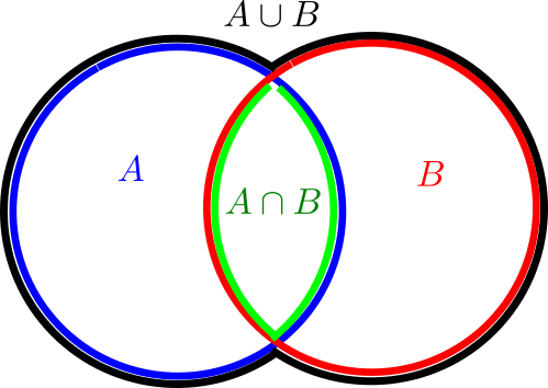
(where we have given each region depicted a different color, and moved the edges of each region a little away from each other in order to make them all visible separately), but if one wanted to instead depict a situation in which the intersection
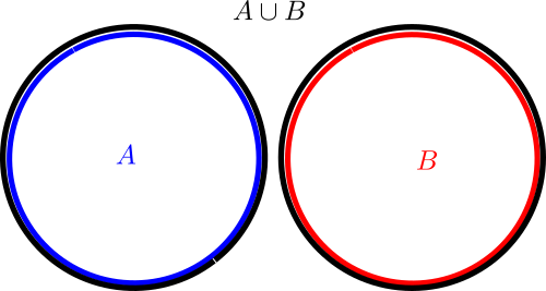
One can use the area of various regions in a Venn or Euler diagram as a heuristic proxy for the cardinality 


 , while the above Euler diagram similarly justifies the special case
  .
.
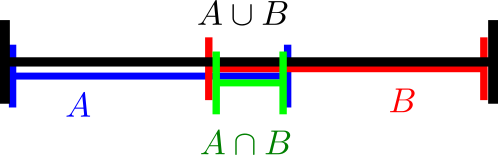
While Venn and Euler diagrams are traditionally two-dimensional in nature, there is nothing preventing one from using one-dimensional diagrams such as
or even three-dimensional diagrams such as this one from Wikipedia:
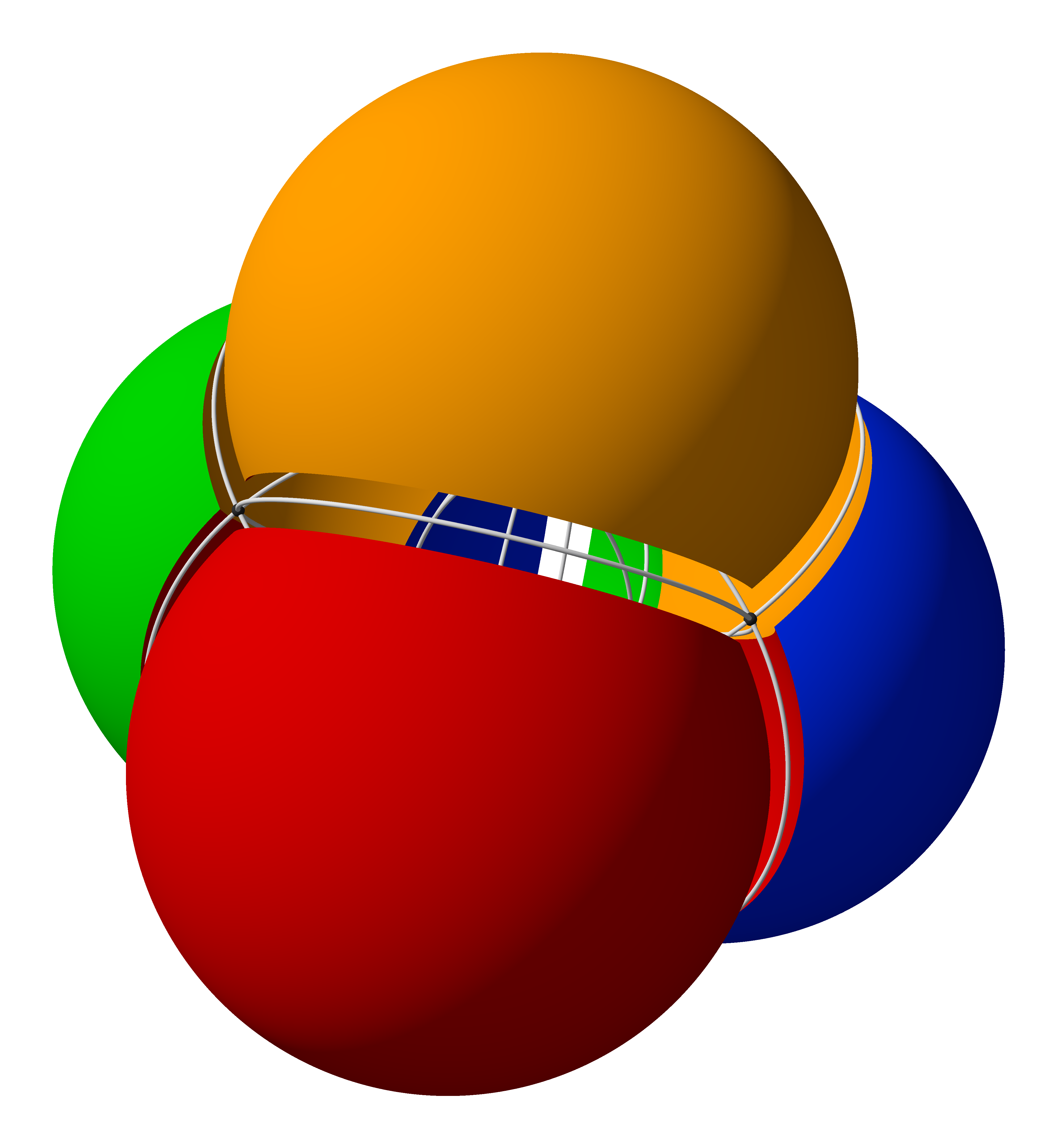
Of course, in such cases one would use length or volume as a heuristic proxy for cardinality or measure, rather than area.
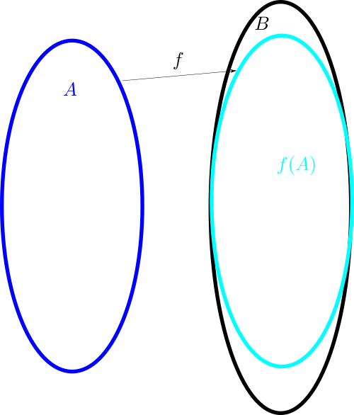
With the addition of arrows, Venn and Euler diagrams can also accommodate (to some extent) functions between sets. Here for instance is a depiction of a function 


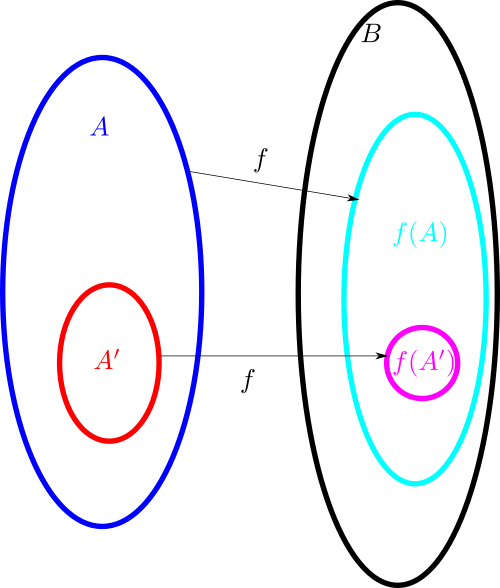
Here one can illustrate surjectivity of 

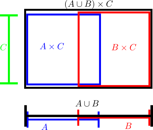
Cartesian product operations can be incorporated into these diagrams by appropriate combinations of one-dimensional and two-dimensional diagrams. Here for instance is a diagram that illustrates the identity 
In this blog post I would like to propose a similar family of diagrams to illustrate relationships between vector spaces (over a fixed base field 

I’m collecting in this blog post a number of simple group-theoretic lemmas, all of the following flavour: if 

- (
of
- (
of
.
- (Structure) There is some useful structural relationship between
.
of a product group , and one needs to know further information about this subgroup in order to take the analysis further. In some cases only two of the above three options are relevant. In the cases where is too “small” or too “large” one can reduce the groups to something smaller (either a subgroup or a quotient) and in applications one can often proceed in this case by some induction on the “size” of the groups (for instance, if these groups are Lie groups, one can often perform an induction on dimension), so it is often the structured case which is the most interesting case to deal with.
It is perhaps easiest to explain the flavour of these lemmas with some simple examples, starting with the 

Lemma 1 Let
- (i) (
into a group
such that
for all
.
- (ii) (
of
Proof: Let 


Here is a “dual” to the above lemma:
Lemma 2 Let
- (i) (
of some subgroup
of
for some non-trivial normal subgroup
of
is the quotient map.
- (ii) (
.
Proof: Let 
For subgroups of nilpotent groups, we have a nice dichotomy that detects properness of a subgroup through abelian representations:
Lemma 3 Let
- (i) (
such that
for all
- (ii)
.
Informally: if
Proof: By definition of nilpotency, the lower central series
![\displaystyle G_2 := [G,G], G_3 := [G,G_2], \dots](https://s0.wp.com/latex.php?latex=%5Cdisplaystyle++G_2+%3A%3D+%5BG%2CG%5D%2C+G_3+%3A%3D+%5BG%2CG_2%5D%2C+%5Cdots&bg=ffffff&fg=000000&s=0&c=20201002)
Since 


![\displaystyle G_2 = [G,G] = [G, HG_2].](https://s0.wp.com/latex.php?latex=%5Cdisplaystyle++G_2+%3D+%5BG%2CG%5D+%3D+%5BG%2C+HG_2%5D.&bg=ffffff&fg=000000&s=0&c=20201002)
 , commutes with , hence
 ![\displaystyle [G, HG_2] \subset [G,H] G_3 \subset H G_3](https://s0.wp.com/latex.php?latex=%5Cdisplaystyle++%5BG%2C+HG_2%5D+%5Csubset+%5BG%2CH%5D+G_3+%5Csubset+H+G_3&bg=ffffff&fg=000000&s=0&c=20201002)

 . One can continue this argument by induction to show that
  for every
  ; taking large enough we end up in option (ii). Finally, it is clear that (i) and (ii) cannot both hold.
Remark 4 When the group. Thus
Here is an analogue of Lemma 3 for special linear groups, due to Serre (IV-23):
Lemma 5 Letbe a prime, and let
, where
is the ring of
-adic integers. Then exactly one of the following hold:
- (i) (
such that
for all
- (ii)
.
Proof: It is a standard fact that the reduction of
Suppose that (i) fails, then for every 


 and , there exists
  with
with  ; taking limits as
  using the closed nature of will then place us in option (ii).
The case 


First suppose that 


Any 


Now suppose 


We note a generalisation of Lemma 3 that involves two groups 
Lemma 6 Letof two nilpotent groups
. Then exactly one of the following hold:
- (i) (
,
into an abelian group
non-trivial, such that
for all
, where
is the projection of
.
- (ii)
for some subgroup
of
Proof: Consider the group 


Finally, it is clear that (i) and (ii) cannot both hold, since (i) places a non-trivial constraint on the second component 
We also note a similar variant of Lemma 5, which is Lemme 10 of this paper of Serre:
Lemma 7 Let. Then exactly one of the following hold:
- (i) (
such that
- (ii)
.
Proof: As in the proof of Lemma 5, (i) and (ii) cannot both hold. Suppose that (i) does not hold, then for any 


The most famous result of this type is of course the Goursat lemma, which we phrase here in a somewhat idiosyncratic manner to conform to the pattern of the other lemmas in this post:
Lemma 8 (Goursat lemma) Let
- (i) (
for some subgroups
of
or
(or both).
- (ii) (
of
, where
is the quotient map.
- (iii) (Isomorphism) There is a group isomorphism
such that
is the graph of
. In particular,
Here we almost have a trichotomy, because option (iii) is incompatible with both option (i) and option (ii). However, it is possible for options (i) and (ii) to simultaneously hold.
Proof: If either of the projections 


Next, if either of the maps 

The only remaining case is when the group homomorphisms 

We can combine the Goursat lemma with Lemma 3 to obtain a variant:
Corollary 9 (Nilpotent Goursat lemma) Let
- (i) (
and a non-trivial group homomorphism
such that
for all
- (ii) (
- (iii) (Isomorphism) There is a group isomorphism
Proof: If Lemma 8(i) holds, then by applying Lemma 3 we arrive at our current option (i). The other options are unchanged from Lemma 8, giving the claim.
Now we present a lemma involving three groups 
Lemma 10 (Furstenberg-Weiss lemma) Letof three groups
. Then one of the following hold:
- (i) (
of
whenever
and
.
- (ii) (
of
abelian, such that
, where
is the quotient map.
- (iii)
Proof: If the group 


 be any two elements of . By the above assumptions, we can find
  such that

 terms, we conclude that
 ![\displaystyle (1, 1, [g_3,g'_3]) \in H.](https://s0.wp.com/latex.php?latex=%5Cdisplaystyle++%281%2C+1%2C+%5Bg_3%2Cg%27_3%5D%29+%5Cin+H.&bg=ffffff&fg=000000&s=0&c=20201002)
 contains every commutator
 ![{[g_3,g'_3]}](https://s0.wp.com/latex.php?latex=%7B%5Bg_3%2Cg%27_3%5D%7D&bg=ffffff&fg=000000&s=0&c=20201002) , and thus contains the entire group
, and thus contains the entire group ![{[G_3,G_3]}](https://s0.wp.com/latex.php?latex=%7B%5BG_3%2CG_3%5D%7D&bg=ffffff&fg=000000&s=0&c=20201002) generated by these commutators. If fails to be abelian, then is a non-trivial normal subgroup of , and now arises from
generated by these commutators. If fails to be abelian, then is a non-trivial normal subgroup of , and now arises from ![{G_1 \times G_2 \times G_3/[G_3,G_3]}](https://s0.wp.com/latex.php?latex=%7BG_1+%5Ctimes+G_2+%5Ctimes+G_3%2F%5BG_3%2CG_3%5D%7D&bg=ffffff&fg=000000&s=0&c=20201002) in the obvious fashion, placing one in option (ii). Hence the only remaining case is when is abelian, giving us option (iii).
in the obvious fashion, placing one in option (ii). Hence the only remaining case is when is abelian, giving us option (iii).
As before, we can combine this with previous lemmas to obtain a variant in the nilpotent case:
Lemma 11 (Nilpotent Furstenberg-Weiss lemma) Let
- (i) (
,
for some abelian group
non-trivial, such that
whenever
is the projection of
.
- (ii) (
- (iii)
Informally, this lemma asserts that if 

Proof: Applying Lemma 10, we are already done if conclusions (ii) or (iii) of that lemma hold, so suppose instead that conclusion (i) holds for say 


The Furstenberg-Weiss argument is often used (though not precisely in this form) to establish that certain key structure groups arising in ergodic theory are abelian; see for instance Proposition 6.3(1) of this paper of Host and Kra for an example.
One can get more structural control on
Lemma 12 (Variant of Furstenberg-Weiss lemma) Let
- (i) (
of
for some
such that
whenever
- (ii) (
of
, where
is the quotient map.
- (iii)
,
,
to an abelian group

The ability to encode an abelian additive relation in terms of group-theoretic properties is vaguely reminiscent of the group configuration theorem.
Proof: We apply Lemma 10. Option (i) of that lemma implies option (i) of the current lemma, and similarly for option (ii), so we may assume without loss of generality that
We may assume that the projections of 


If 


Combining this lemma with Lemma 3, we obtain a nilpotent version:
Corollary 13 (Variant of nilpotent Furstenberg-Weiss lemma) Let
- (i) (
to some abelian group
for some
not both trivial, such that
whenever
- (ii) (
- (iii)
Here is another variant of the Furstenberg-Weiss lemma, attributed to Serre by Ribet (see Lemma 3.3):
Lemma 14 (Serre’s lemma) Let. Then one of the following hold:
- (i) (
such that
.
- (ii) (
.
- (iii) One of the
.
Proof: The claim is trivial for 

![{G_i = [G_i,G_i]}](https://s0.wp.com/latex.php?latex=%7BG_i+%3D+%5BG_i%2CG_i%5D%7D&bg=ffffff&fg=000000&s=0&c=20201002)
We now claim that for any 


![{g_k = [g'_k, g''_k]}](https://s0.wp.com/latex.php?latex=%7Bg_k+%3D+%5Bg%27_k%2C+g%27%27_k%5D%7D&bg=ffffff&fg=000000&s=0&c=20201002)


Setting 

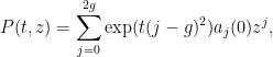
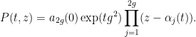
In a recent post I discussed how the Riemann zeta function 
![{t \in [T,2T]}](https://s0.wp.com/latex.php?latex=%7Bt+%5Cin+%5BT%2C2T%5D%7D&bg=ffffff&fg=000000&s=0&c=20201002)

where 


Here 


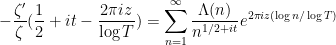
Taking logarithmic derivatives of (2), we have

and hence on taking logarithmic derivatives of (1) in the 

Morally speaking, we have
so on comparing coefficients we expect to interpret the moments 
To understand the distribution of

where 


where 

The moment (6) vanishes unless one has the homogeneity condition

This follows from the fact that for any phase 


In the case when the degree 
Proposition 1 (Low moments in CUE model) If
then the moment (6) vanishes unless
for all
, in which case it is equal to


Another way of viewing this proposition is that for 

Proof: Let 

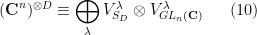
Our starting point is Schur-Weyl duality. Namely, we consider the 

This space has an action of the product group 


where 


Let 


The trace of this action can then be computed as
where 


But we can also compute this trace using the Schur-Weyl decomposition (10), yielding the identity

where 


and similarly

where 


Now recall that 


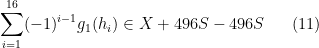
Example 2 We illustrate the identity (11) when
,
. The Schur polynomials are given as
where
are the (generalised) eigenvalues of
The functions
are orthonormal on
are also, and their
norms are
,
, and
respectively, reflecting the size in
of the centralisers of the permutations
,
, and
respectively. If
, then the
terms now disappear (the Young tableau here has too many rows), and the three quantities here now have some non-trivial covariance.


Example 3 Consider the moment
. For
, the above proposition shows us that this moment is equal to
? The formula (12) computes this moment as
where
, and
vanishes unless
of vectors in
whose coordinates sum to zero), in which case it is equal to
(depending on the parity of the number of non-zero rows). As such we see that this moment is equal to


Now we discuss what is known for the analogous moments (5). Here we shall be rather non-rigorous, in particular ignoring an annoying “Archimedean” issue that the product of the ranges 


![{[T,2T]}](https://s0.wp.com/latex.php?latex=%7B%5BT%2C2T%5D%7D&bg=ffffff&fg=000000&s=0&c=20201002)
One can morally expand out (5) using (4) as


where 


for 

for 

in which case the expecation is oscillates with magnitude one. In particular, if (7) fails (with some room to spare) then the moment (5) should be negligible, which is consistent with the analogous behaviour for the moments (6). Now suppose that (8) holds (with some room to spare). Then 


The von Mangoldt factors 


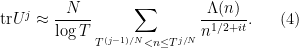
and using Mertens’ theorem this soon simplifies asymptotically to the same quantity in Proposition 1. Thus we see that (morally at least) the moments (5) associated to the zeta function asymptotically match the moments (6) coming from the CUE model in the low degree case (8), thus lending support to the GUE hypothesis. (These observations are basically due to Rudnick and Sarnak, with the degree
With some rare exceptions (such as those estimates coming from “Kloostermania”), the moment estimates of Rudnick and Sarnak basically represent the state of the art for what is known for the moments (5). For instance, Montgomery’s pair correlation conjecture, in our language, is basically the analogue of (13) for 

for all
These estimates can be used to give some non-trivial information on the largest and smallest spacings between zeroes of the zeta function, which in our notation corresponds to spacing between eigenvalues of 


then the arcs 


for sufficiently small 


It would be of great interest if one could push the upper bound 


Unfortunately, the known methods do not seem to break this barrier without some significant new input; already the original paper of Montgomery and Odlyzko observed this limitation for their particular technique (and in fact fall very slightly short, as observed in unpublished work of Goldston and of Milinovich). In this post I would like to record another way to see this, by providing an “alternative” probability distribution to the CUE distribution (which one might dub the Alternative Circular Unitary Ensemble (ACUE) which is indistinguishable in low moments in the sense that the expectation 
To describe this alternative distribution, let us first recall the Weyl description of the CUE measure on the unitary group 
where

is the Vandermonde determinant; see for instance this previous blog post for the derivation of a very similar formula for the GUE distribution, which can be adapted to CUE without much difficulty. To see that this is a probability measure, first observe the Vandermonde determinant identity

where 


For the alternative distribution, we first draw 


shift by a phase 


From construction it is clear that the matrix

when 


By Fourier decomposition, it then suffices to show that the trigonometric polynomial 


Example 4 If
, then the distribution (21) assigns a probability of
to any pair
that is a permuted rotation of
, and a probability of
to any pair that is a permuted rotation of
. Thus, a matrix
with probability
with probability
A similar computation when
gives
with probability
, to a phase rotation of
or its adjoint with probability of
each, and a phase rotation of
with probability
.
Remark 5 For large
In some cases, even just a tiny improvement in known results would be able to exclude the alternative hypothesis. For instance, if the alternative hypothesis held, then 

which differs from (13) for any 
Remark 6 One can view the CUE as normalised Lebesgue measure on
). One can similarly view ACUE as normalised Lebesgue measure on the (disconnected) smooth submanifold of
(or one can equivalently take
; in a similar spirit, the phases of ACUE eigenvalues, once they are rotated to be
). In particular, the
.
Remark 7 One family of estimates that go beyond the Rudnick-Sarnak family of estimates are twisted moment estimates for the zeta function, such as ones that give asymptotics for
for some small even exponent
(almost always
) and some short Dirichlet polynomial
; see for instance this paper of Bettin, Bui, Li, and Radziwill for some examples of such estimates. The analogous unitary matrix average would be something like
where
to cancel the corresponding powers of
). Unfortunately such averages generally are unable to distinguish the CUE from the ACUE. For instance, if all the coefficients of
of total order less than
, then in terms of the eigenvalue phases
is a linear combination of plane waves
where the frequencies
have coefficients of magnitude less than
is a linear combination of plane waves
is a linear combination of plane waves where the frequencies
by the previous arguments. In other words,


Remark 8 The GUE hypothesis for the zeta function asserts that the average
for any
and any test function
, where
is the Dyson sine kernel and
are the ordinates of zeroes of the zeta function. This corresponds to the CUE distribution for
This is a stronger version of the alternative hypothesis that the spacing between adjacent zeroes is almost always approximately a half-integer multiple of the mean spacing. I do not know of any known moment estimates for Dirichlet series that is able to eliminate this AGUE hypothesis (even assuming GRH). (UPDATE: These facts have also been independently observed in forthcoming work of Lagarias and Rodgers.)


Let 


for all 

for all additive quadruples 


Now suppose that 

for all 

for all additive quadruples
“Trivial” examples of quasimorphisms include the sum of a homomorphism and a bounded function. Are there others? In some cases, the answer is no. For instance, suppose we have a quasimorphism 


In general, one can phrase this problem in the language of group cohomology (discussed in this previous post). Call a map 

for all 


Such functions are called 
If a 
In additive combinatorics, one is often working with functions which only have additive structure a fraction of the time, thus for instance (1) or (3) might only hold “

Theorem 1 Let
, let
be a subset of
, and let
be a function such that
for
additive quadruples
. Then there exists a subset
, a subset
of
, and a function
such that
for all
(thus, the derivative
takes values in
on
), and such that for each
, one has
for
values of
.


Presumably the constants 


Proof: By hypothesis, there are 


Thus, there is a set 


for
Consider the bipartite graph whose vertex sets are two copies of 


and 


Also observe that

Thus, if 


for 

By the pigeonhole principle, this implies that for any fixed 


whenever

This implies that there exists a subset 

for all 

 are such that
By construction of 


and

for 

and hence by (8)

where 
we see that there are only 


whenever (10) holds.
For any 


Then from (11) we have (4). For 
This is a sequel to this previous blog post, in which we discussed the effect of the heat flow evolution
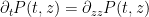
on the zeroes of a time-dependent family of polynomials 

More precisely, let
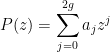
of degree 

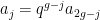
for all 

and
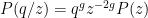
for all non-zero 


Such polynomials arise in number theory as follows: if 


where 


Another key example of such polynomials arise from rescaled characteristic polynomials

of 

Given a polynomial 

we can evolve it in time by the formula
thus 


In view of the results of Marcus, Spielman, and Srivastava, it is also very likely that one can interpret this flow in terms of expected characteristic polynomials involving conjugation over the compact symplectic group 

It is clear that if 


From the inverse function theorem we see that for times 
Differentiating this at any 

and

and

Inserting these formulae into (2) (expanding 


for 

which we can rearrange as

If we make the change of variables 

Intuitively, this equation asserts that the phases 

then the above equation becomes a gradient flow
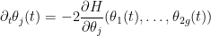
which implies in particular that 


For any polynomial 


For instance, consider the case when 
has zeroes

and one easily checks that these zeroes lie on the circle 


The arguments in my paper with Brad Rodgers (discussed in this previous post) indicate that for a “typical” polynomial 

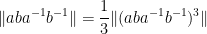
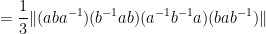
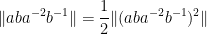
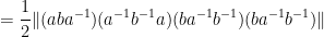
The Polymath14 online collaboration has uploaded to the arXiv its paper “Homogeneous length functions on groups“, submitted to Algebra & Number Theory. The paper completely classifies homogeneous length functions 


The proof is based on repeated use of the homogeneous length function axioms, combined with elementary identities of commutators, to obtain increasingly good bounds on quantities such as ![{\|[x,y]\|}](https://s0.wp.com/latex.php?latex=%7B%5C%7C%5Bx%2Cy%5D%5C%7C%7D&bg=ffffff&fg=000000&s=0&c=20201002)
As there are now a large number of comments on the previous post on this project, this post will also serve as the new thread for any final discussion of this project as it winds down.
In the tradition of “Polymath projects“, the problem posed in the previous two blog posts has now been solved, thanks to the cumulative effect of many small contributions by many participants (including, but not limited to, Sean Eberhard, Tobias Fritz, Siddharta Gadgil, Tobias Hartnick, Chris Jerdonek, Apoorva Khare, Antonio Machiavelo, Pace Nielsen, Andy Putman, Will Sawin, Alexander Shamov, Lior Silberman, and David Speyer). In this post I’ll write down a streamlined resolution, eliding a number of important but ultimately removable partial steps and insights made by the above contributors en route to the solution.
Theorem 1 Let
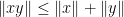
be a group. Suppose one has a “seminorm” function
which obeys the triangle inequality
for all
. Then the seminorm factors through the abelianisation map
.
Proof: By the triangle inequality, it suffices to show that ![{\| [x,y]\| = 0}](https://s0.wp.com/latex.php?latex=%7B%5C%7C+%5Bx%2Cy%5D%5C%7C+%3D+0%7D&bg=ffffff&fg=000000&s=0&c=20201002)
![{[x,y] := xyx^{-1}y^{-1}}](https://s0.wp.com/latex.php?latex=%7B%5Bx%2Cy%5D+%3A%3D+xyx%5E%7B-1%7Dy%5E%7B-1%7D%7D&bg=ffffff&fg=000000&s=0&c=20201002)
We first establish some basic facts. Firstly, by hypothesis we have 


for all 


Next, for any

so on taking limits as 


Next, we observe that if 


Indeed, if we write 


where the 

and the claim (3) follows by sending
The following special case of (3) will be of particular interest. Let 
![\displaystyle f(m,k) := \| x^m [x,y]^k \|.](https://s0.wp.com/latex.php?latex=%5Cdisplaystyle+f%28m%2Ck%29+%3A%3D+%5C%7C+x%5Em+%5Bx%2Cy%5D%5Ek+%5C%7C.&bg=ffffff&fg=000000&s=0&c=20201002)
Observe that ![{x^m [x,y]^k}](https://s0.wp.com/latex.php?latex=%7Bx%5Em+%5Bx%2Cy%5D%5Ek%7D&bg=ffffff&fg=000000&s=0&c=20201002)
![{x (x^{m-1} [x,y]^k)}](https://s0.wp.com/latex.php?latex=%7Bx+%28x%5E%7Bm-1%7D+%5Bx%2Cy%5D%5Ek%29%7D&bg=ffffff&fg=000000&s=0&c=20201002)
![{(y^{-1} x^m [x,y]^{k-1} xy) x^{-1}}](https://s0.wp.com/latex.php?latex=%7B%28y%5E%7B-1%7D+x%5Em+%5Bx%2Cy%5D%5E%7Bk-1%7D+xy%29+x%5E%7B-1%7D%7D&bg=ffffff&fg=000000&s=0&c=20201002)
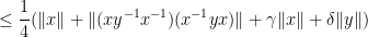
![\displaystyle \| x^m [x,y]^k \| \leq \frac{1}{2} ( \| x^{m-1} [x,y]^k \| + \| y^{-1} x^{m} [x,y]^{k-1} xy \|)](https://s0.wp.com/latex.php?latex=%5Cdisplaystyle+%5C%7C+x%5Em+%5Bx%2Cy%5D%5Ek+%5C%7C+%5Cleq+%5Cfrac%7B1%7D%7B2%7D+%28+%5C%7C+x%5E%7Bm-1%7D+%5Bx%2Cy%5D%5Ek+%5C%7C+%2B+%5C%7C+y%5E%7B-1%7D+x%5E%7Bm%7D+%5Bx%2Cy%5D%5E%7Bk-1%7D+xy+%5C%7C%29&bg=ffffff&fg=000000&s=0&c=20201002)
which by (2) leads to the recursive inequality

We can write this in probabilistic notation as

where 

where 


![\displaystyle f( Z ) \leq |Y_1+\dots+Y_{2n}| (\|x\| + \frac{1}{2} \| [x,y] \|),](https://s0.wp.com/latex.php?latex=%5Cdisplaystyle+f%28+Z+%29+%5Cleq+%7CY_1%2B%5Cdots%2BY_%7B2n%7D%7C+%28%5C%7Cx%5C%7C+%2B+%5Cfrac%7B1%7D%7B2%7D+%5C%7C+%5Bx%2Cy%5D+%5C%7C%29%2C&bg=ffffff&fg=000000&s=0&c=20201002)
noting that 

![\displaystyle f(0,n) \leq \sqrt{2n}( \|x\| + \frac{1}{2} \| [x,y] \|).](https://s0.wp.com/latex.php?latex=%5Cdisplaystyle+f%280%2Cn%29+%5Cleq+%5Csqrt%7B2n%7D%28+%5C%7Cx%5C%7C+%2B+%5Cfrac%7B1%7D%7B2%7D+%5C%7C+%5Bx%2Cy%5D+%5C%7C%29.&bg=ffffff&fg=000000&s=0&c=20201002)
But by (1), the left-hand side is equal to ![{n \| [x,y]\|}](https://s0.wp.com/latex.php?latex=%7Bn+%5C%7C+%5Bx%2Cy%5D%5C%7C%7D&bg=ffffff&fg=000000&s=0&c=20201002)
The above theorem reduces such seminorms to abelian groups. It is easy to see from (1) that any torsion element of such groups has zero seminorm, so we can in fact restrict to torsion-free groups, which we now write using additive notation 


This post is a continuation of the previous post, which has attracted a large number of comments. I’m recording here some calculations that arose from those comments (particularly those of Pace Nielsen, Lior Silberman, Tobias Fritz, and Apoorva Khare). Please feel free to either continue these calculations or to discuss other approaches to the problem, such as those mentioned in the remaining comments to the previous post.
Let 


and the linear growth property

for all 

or equivalently

We consider inequalities of the form


for various real numbers 

we have (1) for 
Proposition 1
 .
. , then
  .
. .
.Proof: For (i) we simply observe that

For (ii), we calculate


giving the claim.
For (iii), we calculate


giving the claim.
For (iv), we calculate


giving the claim.
Here is a typical application of the above estimates. If (1) holds for 


For instance, if 

Here is a curious question posed to me by Apoorva Khare that I do not know the answer to. Let
- bi-invariant, thus
for all
; and
- linear growth in the sense that
for all
and all natural numbers
By defining the “norm” of an element 
for all 

for all
for all 
One can normalise the norm of the generators to be at most

This can then be used to upper bound the norm of other words in

A bit less trivially, from (3), (2), (1) one can bound commutators as

In a similar spirit one has

What is not clear to me is if one can keep arguing like this to continually improve the upper bounds on the norm 
How many groups of order four are there? Technically, there are an enormous number, so much so, in fact, that the class of groups of order four is not even a set, but merely a proper class. This is because any four objects 


A much better question is to ask how many groups of order four there are up to isomorphism, counting each isomorphism class of groups exactly once. Now, as one learns in undergraduate group theory classes, the answer is just “two”: the cyclic group 

More generally, given a class of objects 


![{[x]:=\{y\in X:x \sim {}y \}}](https://s0.wp.com/latex.php?latex=%7B%5Bx%5D%3A%3D%5C%7By%5Cin+X%3Ax+%5Csim+%7B%7Dy+%5C%7D%7D&bg=ffffff&fg=000000&s=0&c=20201002)
![\displaystyle |X/\sim| = \sum_{x \in X} \frac{1}{|[x]|}, \ \ \ \ \ (1)](https://s0.wp.com/latex.php?latex=%5Cdisplaystyle+%7CX%2F%5Csim%7C+%3D+%5Csum_%7Bx+%5Cin+X%7D+%5Cfrac%7B1%7D%7B%7C%5Bx%5D%7C%7D%2C+%5C+%5C+%5C+%5C+%5C+%281%29&bg=ffffff&fg=000000&s=0&c=20201002)
thus one counts elements in
Example 1 Let
of integers between
and
of
. Then the quotient space
,
, and
. Thus there are three objects in
Thus, to count elements in
are given a weight of
Given a finite probability set 

Given a notion ![{[\mathbf{x}] \in X/\sim}](https://s0.wp.com/latex.php?latex=%7B%5B%5Cmathbf%7Bx%7D%5D+%5Cin+X%2F%5Csim%7D&bg=ffffff&fg=000000&s=0&c=20201002)

![{[\mathbf{x}]}](https://s0.wp.com/latex.php?latex=%7B%5B%5Cmathbf%7Bx%7D%5D%7D&bg=ffffff&fg=000000&s=0&c=20201002)


However, it is possible to remove this bias by changing the weighting in (1), and thus changing the notion of what cardinality means. To do this, we generalise the previous situation. Instead of considering sets
Definition 2 A groupoid is a set (or proper class)
of “isomorphisms” between any pair
from isomorphisms
,
to isomorphisms in
for every
, obeying the following group-like axioms:
- (Identity) For every
, there is an identity isomorphism
, such that
for all
.
- (Associativity) If
for some
, then
.
- (Inverse) If
such that
and
.
We say that two elements
, if there is at least one isomorphism from
.
Example 3 Any category gives a groupoid by taking
of sets,
of linear vector spaces over some given base field
Every set 


However, one can also form multiply-connected groupoids in which there can be multiple isomorphisms from one element of 


For a finite multiply-connected groupoid, it turns out that the natural notion of “cardinality” (or as I prefer to call it, “cardinality up to isomorphism”) is given by the variant

of (1). That is to say, in the multiply connected case, the denominator is no longer the number of objects ![{[x]}](https://s0.wp.com/latex.php?latex=%7B%5Bx%5D%7D&bg=ffffff&fg=000000&s=0&c=20201002)
![\displaystyle \sum_{[x] \in X/\sim} \frac{1}{|\mathrm{Aut}(x)|} \ \ \ \ \ (2)](https://s0.wp.com/latex.php?latex=%5Cdisplaystyle+%5Csum_%7B%5Bx%5D+%5Cin+X%2F%5Csim%7D+%5Cfrac%7B1%7D%7B%7C%5Cmathrm%7BAut%7D%28x%29%7C%7D+%5C+%5C+%5C+%5C+%5C+%282%29&bg=ffffff&fg=000000&s=0&c=20201002)
where 


For instance, if we take
exactly as before. If however we take the multiply connected groupoid on

the equivalence class ![{[0]}](https://s0.wp.com/latex.php?latex=%7B%5B0%5D%7D&bg=ffffff&fg=000000&s=0&c=20201002)
![{[1], [2]}](https://s0.wp.com/latex.php?latex=%7B%5B1%5D%2C+%5B2%5D%7D&bg=ffffff&fg=000000&s=0&c=20201002)


The definition (2) can also make sense for some infinite groupoids; to my knowledge this was first explicitly done in this paper of Baez and Dolan. Consider for instance the category 


(This fact is sometimes loosely stated as “the number of finite sets is 

because the cyclic group
In the case that the cardinality of a groupoid
![\displaystyle {\mathbf P}([\mathbf{x}] = [x]) = \frac{1 / |\mathrm{Aut}(x)|}{\sum_{[y] \in X/\sim} 1/|\mathrm{Aut}(y)|},](https://s0.wp.com/latex.php?latex=%5Cdisplaystyle+%7B%5Cmathbf+P%7D%28%5B%5Cmathbf%7Bx%7D%5D+%3D+%5Bx%5D%29+%3D+%5Cfrac%7B1+%2F+%7C%5Cmathrm%7BAut%7D%28x%29%7C%7D%7B%5Csum_%7B%5By%5D+%5Cin+X%2F%5Csim%7D+1%2F%7C%5Cmathrm%7BAut%7D%28y%29%7C%7D%2C&bg=ffffff&fg=000000&s=0&c=20201002)
thus the probability of being isomorphic to a given element ![{[0], [1], [2]}](https://s0.wp.com/latex.php?latex=%7B%5B0%5D%2C+%5B1%5D%2C+%5B2%5D%7D&bg=ffffff&fg=000000&s=0&c=20201002)
![{[1]}](https://s0.wp.com/latex.php?latex=%7B%5B1%5D%7D&bg=ffffff&fg=000000&s=0&c=20201002)
![{[2]}](https://s0.wp.com/latex.php?latex=%7B%5B2%5D%7D&bg=ffffff&fg=000000&s=0&c=20201002)

Using the groupoid of finite sets, we see that a finite set chosen uniformly up to isomorphism will have a cardinality that is distributed according to the Poisson distribution of parameter 
One important source of groupoids are the fundamental groupoids 

where 


This notion of cardinality up to isomorphism of a groupoid behaves well with respect to various basic notions. For instance, suppose one has an 


![{[\mathrm{x}]}](https://s0.wp.com/latex.php?latex=%7B%5B%5Cmathrm%7Bx%7D%5D%7D&bg=ffffff&fg=000000&s=0&c=20201002)
![{\pi([\mathrm{x}])}](https://s0.wp.com/latex.php?latex=%7B%5Cpi%28%5B%5Cmathrm%7Bx%7D%5D%29%7D&bg=ffffff&fg=000000&s=0&c=20201002)
Indeed, one can show that this notion of cardinality up to isomorphism for groupoids is uniquely determined by a small number of axioms such as these (similar to the axioms that determine Euler characteristic); see this blog post of Qiaochu Yuan for details.
The probability distributions on isomorphism classes described by the above recipe seem to arise naturally in many applications. For instance, if one draws a profinite abelian group up to isomorphism at random in this fashion (so that each isomorphism class ![{[G]}](https://s0.wp.com/latex.php?latex=%7B%5BG%5D%7D&bg=ffffff&fg=000000&s=0&c=20201002)

Recent Comments